Should We Care About the Uncertainty Around
Measures of Political-Economic Development?
Rodolphe Desbordes
‡Gary Koop
§Abstract
Several proxies of political-economic development, such as the Worldwide Governance
Indicators, come in the form of an estimate along with a standard error reflecting the
un-certainty of this estimate. Existing empirical work discards the information provided by
the standard errors. We argue that the appropriate practice should be to take into account
this additional information through the use of multiple imputation. We investigate the
importance of our proposed approach in several applications. We find that accounting
for the uncertainty around the values of various measures of political-economic
develop-ment tends to have a large influence on the magnitude and statistical significance of the
estimated effects of these variables.
JEL classification: C1, F1, F2, O11. Keywords: democracy; income inequality;
gover-nance; multiple imputation; uncertainty.
‡Corresponding author. University of Strathclyde. Address: Department of Economics, Sir William
Dun-can Building, University of Strathclyde, 130 Rottenrow, Glasgow G4 0GE, Scotland, United Kingdom. Tele-phone/Fax number: +44 141 548 3961/+44 141 548 5776. E-mail: rodolphe.desbordes@strath.ac.uk
1
Introduction
In the economic growth and development literature it is common to use proxies for key mea-sures of political-economic development such as governance or democracy. For example, the Worldwide Governance Indicators (WGI) are widely used to assess institutional quality (see Kaufmann et al. (1999, 2011)). The WGI project provides quantitative information on six dimensions of governance, by averaging in a statistically sophisticated manner a very large number of underlying variables coming from thirty-two independent data sources. The es-timates provided are commonly included in econometric models. The creators of the WGI (and the creators of aggregate governance indicators based on extensions of the WGI method-ology) have consistently stressed the uncertainty of their governance estimates and provide a standard error for each estimate. Several papers have used these standard errors in empirical exercises such as interpreting country rankings (see, e.g., Kaufmann and Kraay (2002), Treis-man (2007), Høyland et al. (2012), and Standaert (forthcoming)). However, to our knowl-edge, no use has been made of the information in the WGI standard errors in the regressions and panel data models that are the main econometric tools used in the growth and develop-ment literatures. This paper aims to fill this gap. We use multiple imputation methods to investigate whether failing to take into account the information on the uncertainty of WGI and other measures of political-economic development is an important issue.
development has, in some cases, a large influence on empirical results.
The remainder of this paper is organized as follows. Section 2 describes our econometric approach. Section 3 presents our applications. Section 4 concludes.
2
Generated Variables and Multiple Imputation
Generated variables are those constructed using a first-step model which are then used in a regression. A standard practice is to bootstrap the standard errors of the parameter esti-mates, in order to take into account the fact that generated variables are measured with error (Wooldridge, 2010). In the absence of additional information, this is certainly the best that the researcher can do. However, for some variables, such as the WGI, uncertainty about their values is provided, in the form of standard errors. This additional information can be exploited, as we explain below.
To describe the main issues, consider a regression model with dependent variable, y, explanatory variable,x∗, coefficientsβ and error varianceσ2. Subscriptsi= 1, .., N denote individual observations. Our proxy forx∗
i is the generated regressorxiandx∗i ∼N xi, σxi2
.1 For some variables, such as those produced by the WGI project, standard errors, σxi2 , are provided. Researchers usually focus onxionly. However, a natural way to take into account
the information provided byσxi2 is to adopt a Bayesian perspective where inference is based on a posterior density (i.e. a density for any model parameters conditional on the data set). Ideally, we wish to have inference based on the posterior conditional on the true value of the
1This interpretation is consistent with Kaufmann et al. (2009) which states on page 16: “the output of our
explanatory variable:p(β, σ2|y, x∗). However,x∗ is not known with certainty. All we know is the distribution ofx∗ conditional on the information that was used to compute the WGI (call thisz): p(x∗|z). Thus, we need to work with the posterior: p(β, σ2|y, z). Given the structure of our problem, wherez is only used to construct the WGI variables and does not directly enter the regression, this posterior can be written as:
p β, σ2|y, z
=
Z
p β, σ2|y, x∗
p(x∗|z)dx∗. (1)
As outlined below, multiple imputation can be used to calculate this posterior. In contrast, a researcher who ignores the uncertainty about the WGI and usesxas an explanatory variable bases inference on the posterior:
p β, σ2|y, x
=p β, σ2|y, x∗ =x
. (2)
Put simply,p(β, σ2|y, z)and p(β, σ2|y, x)are different posteriors and, hence, the will lead to different inference. The exact relationship between these two posterior is theoretically unclear. We might expect them to be similar to one another, but withp(β, σ2|y, z) leading
to larger measures of dispersion than p(β, σ2|y, x) due to the incorporation of the uncer-tainty surrounding the WGI variables. We often do find this result, but theoretically other outcomes are possible and a purpose of this paper is to investigate how much p(β, σ2|y, z)
andp(β, σ2|y, x)diverge from one another in practice.
In order to draw inference onp(β, σ2|y, z)we need to evaluate the integral in (1). This can be done using an averaging procedure, where many regressions have been run, using different plausible values of the variable of interest. In our case, the fact that the WGI project provides us withp(x∗|z)means that the averaging can be done in a very simple fashion:
i Simulates= 1, .., S drawsx∗(s)
i fori= 1, .., N from theN xi, σxi2
ii For each of these draws, use the posteriorp β, σ2|y, x∗(s)to carry out the desired econo-metric inference.
iii Average inferences over allS estimates produced in step 2.
The strategy outlined in the three steps also goes by the name of multiple imputation and the draws of Step 1 are called imputations. Multiple imputation was developed as a tool for estimating a variety of models where variables have missing values (see, e.g., Rubin (1996)). The use of generated variables can be interpreted as a kind of missing data problem (i.e. where the variable of interest,x∗, is missing but information is known about its distribution).
Bayesian econometrics have gained in popularity in the last two decades but the fre-quentist paradigm still dominates the empirical literature. Fortunately, multiple imputation is compatible with frequentist estimators and can be implemented in standard econometric software like Stata.2 For the frequentist, values ofx∗
i can still be imputed as in step 1 and
used in a multiple imputation procedure. The only difference with the Bayesian approach that we outlined above is that a frequentist estimator is used in step 2.
To summarize, the existing empirical literature uses xi as proxy variable. This does not
lead to inconsistent estimators of the parameters but such a procedure, including when it involves parametric bootstrap, ignores the uncertainty in the proxy variable. Ideally, one would want to use the entire distribution of x∗
i as the proxy variable, given that it contains
useful information about the uncertainty associated with calculating the generated values, and notxi. Multiple imputation is a method which allows us to do this. In practice, results
produced using multiple imputation can differ markedly from non-multiply-imputed results, even if the latter are not inconsistent. It is worth stressing that multiple imputation influences both point estimates and standard errors, although the direction of influence is theoretically
unclear. In other words, estimates and standard errors could either be smaller or larger than those produced without multiple imputation.3
So far, we have discussed the econometric theory when there is a single, cross-sectional explanatory variable, x∗
i. The researcher may want to multiply impute several explanatory
variables. In such a case, we would want to allow for the fact that they could be correlated with one another (e.g. if they were derived from over-lapping data sources). Similarly, in panel or time series contexts, we would want to allow for the fact that imputations of a given variable at different time periods may be correlated with one another. The WGI data set we use does not allow us to handle either type of correlation and we are implicitly assuming our multiply-imputed variables are independent of each other and over time. Standaert (forth-coming) discusses both these issues and their consequences in detail. In particular, he shows that the value of a WGI for an individual country can be highly autocorrelated over time. He demonstrates that when this fact is ignored, the significance of changes over time in a country’s WGI will be under-estimated. Intuitively, for a given country, imputations for two different time periods should be taken from a bivariate distribution with a positive correlation. The positive correlation will increase the chances of imputing similar values for the WGI in the two time periods. By implicitly assuming a zero correlation, our panel data applications are missing this feature and are using imputations that are less similar (across time) than they should be. A similar line of reasoning implies that, in our application which uses more than one WGI indicator, the correlations between our imputed explanatory variables are lower than they should be.
We also note that, in one application, we are imputing an average WGI. At each
impu-3Multiply imputed standard errors involve a within-imputation component (average of variance estimates)
tation we draw from each of the six individual WGI (assuming independence) and average the result. By ignoring the positive correlation between the indicators, we will be under-estimating the uncertainty associated with this average WGI.4
Given the nature of our data, we can only note these issues and suggest the reader keep them in mind when interpreting our results.
3
Empirical applications
In this section, we consider several different empirical applications involving prominent gen-erated political-economic variables, for which estimates and measures of uncertainty such as standard errors are provided. These proxy variables are related to the quality of governance, the democratic nature of a country’s political regime, and the level of income inequality. Each application contains only a brief summary of the relevant aspects of the data. However, Table 6 in Appendix A provides complete definitions, sources and measurement units for all of our variables.
The WGI, which are at the heart of most of our empirical applications, are widely used proxies of political-economic development in the literature. The WGI project reports ag-gregate indicators for six dimensions of public governance: Voice and Accountability (VA); Political Stability (PS); Government Effectiveness (GE); Regulatory Quality (RQ); Rule of Law (RL); Control of Corruption (CC). VA and PS attempt to capture the process by which those in authority are selected and replaced, GE and RQ are related to the ability of the gov-ernment to formulate and implement sound policies, while RL and CC assess the respect of citizens and the state for the institutions which govern them.5 Each indicator is a weighted
4This follows from the fact that, for two random variables, aandb,var(a+b) = var(a) +var(b) +
2cov(a, b). We are instead implicitly assumingvar(a+b) =var(a) +var(b)and working with a variance which is too small.
combination of a large number of different data sources, capturing the views and experiences of survey respondents and experts. Values for each governance indicator range from around -2.5 to 2.5 and are available over the period 1996-2012 for 215 countries.
As emphasized in, e.g., Kaufmann et al. (2011), although the point estimates of the gov-ernance indicators vary substantially across countries and over time, interval estimates can overlap substantially. Overall, there is a high degree of uncertainty of these variables, but not so high as to preclude making meaningful comparisons for many countries either in the cross section (e.g. differences in governance between many pairs of countries are statistically significant) or, to a lesser extent, in the time series dimension (e.g. some countries exhibit statistically significant changes in governance over time).
In our applications, we are interested in finding out whether explicitly accounting for the uncertainty in these estimates will substantially affect empirical results. For each application, we report the standard estimates produced ignoring the generated regressor issue followed by multiple imputation results. For the former, we also provide bootstrapped standard errors in brackets. As expected, these are larger than the uncorrected standard errors, but only rarely to such a degree as to alter conclusions about the statistical significance of coefficients. On the other hand, our empirical applications show that the results produced using multiple imputa-tion often vary substantially from convenimputa-tional estimates, casting doubt on the robustness of findings ignoring uncertainty about various measures of political-economic development.
3.1
Capital flows and governance
3.1.1 Data and empirical approach
that higher institutional quality, as measured by the average of the six WGI, increases inflows and decreases outflows for both debt and equity. These results echo those of Daude and Stein (2007), Alfaro et al. (2008), Faria and Mauro (2009), and Azémar and Desbordes (2013). They have been frequently interpreted as providing a partial answer to the Lucas Paradox. Poor countries do not attract large equity inflows because of the low productivity induced by their poor governance.
In Binici et al. (2010), the dependent variable is the log of financial flows per capita; these financial flows can be equity inflows, debt inflows, equity outflows or debt outflows. The explanatory variables are de jure capital account restrictions, various control variables and the average of the six WGI.6 Like them, we omit oil-exporting countries and keep our sample constant across regressions. Overall, our sample covers 71 countries over the period 1998-2005.7 We re-examine the regressions of Table 3 of their paper. Binici et al. (2010) estimate their log-linearized model using a fixed effects OLS estimator and a sample devoid of zero values. We we do the same. Standard errors are clustered at the country level.
3.1.2 Results
Our results are presented in Table 1. In the upper panel, columns (1)-(4) are regressions the most comparable to those carried out by Binici et al. (2010) in Table 3 of their paper. The multiple imputation results are provided in the lower panel of Table 1 in columns (1’)-(4’).
The results of columns (1-4) mirror, at least in qualitative terms, Binici et al. (2010)’s key
6They use the average of the percentile rank of the six indicators. Thus, we retain cardinal information
which would be lost with ranking. Furthermore, we avoid the possibility of a fall in the percentile rank despite better governance. Finally, percentile ranking is sensitive to the introduction of new countries. Nevertheless, in unreported regressions, we find that our key results are unchanged when we use the average of the percentile rank of the six indicators as the measure of institutional quality.
7They report having data over the period 1995-2005. However, data on debt inflow/outflow restrictions are
Table 1: Capital flows and governance
Debt securities FDI+portfolio equity
Inflow Outflow Inflow Outflow
ln(flow/population); Within estimator
(1) (2) (3) (4)
Average six WGI 1.190* -0.483 1.924*** -1.757***
(0.660) (0.606) (0.714) (0.625)
[0.765] [0.665] [0.745]*** [0.706]**
ln(GDP per cap) 4.796*** 3.395*** 4.184*** 4.951***
(1.302) (0.928) (1.487) (1.383)
[1.415]*** [0.947]*** [1.571]*** [1.494]*** Capital in/out-flow controls -0.354 -0.473* -0.361 -0.644*
(0.344) (0.253) (0.492) (0.357)
[0.393] [0.280]* [0.500] [0.409]
Private credit/GDP 0.131 1.123 0.198 0.836*
(0.707) (0.682) (0.593) (0.487)
[0.792] [0.756] [0.729] [0.526]
STMK CAP/GDP -0.439 -0.151 0.137 0.615**
(0.419) (0.395) (0.447) (0.266)
[0.496] [0.451] [0.509] [0.328]*
(Fuel,Metals,Ore)/Exports -2.831 2.941 3.146 -2.190
(2.891) (2.055) (3.451) (2.360)
[3.207] [2.213] [3.700] [2.552]
Trade openness -1.700** -0.806 -0.964 -0.101
(0.806) (0.564) (0.782) (0.749)
[1.005]* [0.679] [0.980] [0.935]
With WGI uncertainty
(1’) (2’) (3’) (4’)
Average six WGI 0.203 -0.109 0.366 -0.365
(0.410) (0.335) (0.428) (0.387)
ln(GDP per cap) 5.026*** 3.317*** 4.607*** 4.555***
(1.303) (0.942) (1.506) (1.404)
Capital in/out-flow controls -0.468 -0.435 -0.394 -0.645*
(0.348) (0.263) (0.538) (0.356)
Private credit/GDP 0.089 1.142* 0.121 0.909*
(0.726) (0.676) (0.604) (0.495)
STMK CAP/GDP -0.329 -0.193 0.313 0.455
(0.413) (0.404) (0.462) (0.283)
(Fuel,Metals,Ore)/Exports -3.408 3.116 2.204 -1.340
(2.940) (2.070) (3.806) (2.890)
Trade openness -1.705** -0.807 -0.976 -0.083
(0.850) (0.559) (0.842) (0.745)
Observations 300 300 300 300
findings. We find that restrictions on capital outflows appear to be much more effective than restrictions on capital inflows and that higher institutional quality tends to encourage capital inflows and discourage capital inflows.8 However, columns (1’)-(4’) present a very different picture once we take into account the uncertainty with which the governance variables are measured. In all columns, the estimated coefficient on institutional quality becomes much smaller and is no longer statistically significant at conventional levels, despite smaller stan-dard errors.9 Furthermore, the estimated coefficients on some of the non-imputed variables also lose statistical significance, e.g. capital controls in column (2’).
Overall, we find that Binici et al. (2010)’s key findings are not robust to accounting explicitly for the uncertainty of the WGI. Our multiple imputation approach leads to a very large fall in the magnitude of the estimated coefficient on the governance variable, rendering it statistically insignificant. This is possibly because the fixed effects estimator relies solely on time-series variation in the data for identification of the parameters, and, as discussed previously, changes in the WGI can be extremely noisy variables once the uncertainty of these indicators is taken into account.
3.2
International trade and governance
3.2.1 Data and empirical approach
Berden et al. (2014) investigate the impact of governance on international trade.10 They estimate gravity equations in which they include, on the destination (importing) side, the six WGI separately in order to isolate their respective impacts. They find that VA and PS both reduce trade overall, whereas RQ increases it. Other WGI (GE, RL, CC) are not statistically
8Results for the other control variables are also very similar across the two studies.
9These smaller standard errors are likely to be the outcome of greater variation in the data when using
multiple imputation.
significant. They conclude that democracy reduces trade when its main effect is to give more voice to those likely to be affected by international competition, e.g. unskilled workers.11
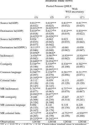
In Berden et al. (2014), the dependent variable corresponds to bilateral exports. The explanatory variables are those which are traditionally found in gravity-type equations (GDP, GDP per capita, bilateral distance, contiguity, common language, colonial history, proxies for multilateral resistance) and the six WGI.12 They use trade data for the period 1997-2004. We simply use all the trade data available in our data source for the same time period. Our dataset includes bilateral trade between 180 countries across five years (1998, 2000, 2002, 2003, 2004). We re-examine one of the main regressions in their paper which is presented in column (6) of their Table 8. In a second stage, we also investigate the impact of exporting countries’ governance on bilateral trade. Like Berden et al. (2014), our estimator is the pooled Poisson quasi-maximum likelihood estimator (QMLE) and standard errors are clustered at the importing country level.
3.2.2 Empirical results
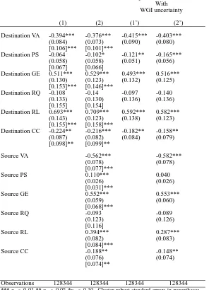
Our results are presented in Tables 2 and 3. Column (1) is the regression the most comparable to that estimated by Berden et al. (2014) in column (6) of Table 8 in their paper. In column (2), we include the WGI on the exporting side. Columns (1’)-(2’) provide the multiple imputation results.
The results of column (1) echo the key finding of Berden et al. (2014): destination VA has a strong, negative, and statistically significant impact on trade.13 On the other hand, we fail
11This result contrasts with previous literature, which has typically found a positive relationship between
democracy and trade openness (Milner and Mukherjee, 2009). The authors argue that is because earlier works did not specifically focus on the pluralism dimension of democracy.
12As in the previous application, the authors use their percentile rank while we use their mean. In unreported
Table 2: Bilateral trade flows and governance
Bilateral trade flows
Pooled Poisson QMLE With WGI uncertainty
(1) (2) (1’) (2’)
Destination VA -0.394*** -0.376*** -0.415*** -0.403***
(0.084) (0.073) (0.090) (0.080)
[0.106]*** [0.101]***
Destination PS -0.064 -0.102* -0.121** -0.165***
(0.058) (0.058) (0.051) (0.056)
[0.067] [0.066]
Destination GE 0.511*** 0.529*** 0.493*** 0.516***
(0.130) (0.123) (0.132) (0.125)
[0.153]*** [0.146]***
Destination RQ -0.108 -0.14 -0.097 -0.140
(0.133) (0.130) (0.136) (0.136)
[0.155] [0.154]
Destination RL 0.693*** 0.709*** 0.592*** 0.582***
(0.143) (0.123) (0.138) (0.123)
[0.155]*** [0.158]***
Destination CC -0.224** -0.216*** -0.182** -0.158**
(0.087) (0.082) (0.084) (0.079)
[0.098]** [0.099]**
Source VA -0.562*** -0.582***
(0.078) (0.078)
[0.077]***
Source PS 0.110*** 0.040
(0.026) (0.026)
[0.031]***
Source GE 0.552*** 0.553***
(0.059) (0.060)
[0.068]***
Source RQ -0.093 -0.089
(0.123) (0.126)
[0.116]
Source RL 0.394*** 0.287***
(0.082) (0.083)
[0.084]***
Source CC -0.188** -0.148**
(0.076) (0.074)
[0.074]**
Observations 128344 128344 128344 128344
Table 3: Bilateral trade flows and governance, continued
Bilateral trade flows
Pooled Poisson QMLE With WGI uncertainty
(1) (2) (1’) (2’)
Source ln(GDP) 0.813*** 0.818*** 0.815*** 0.817***
(0.032) (0.025) (0.032) (0.025)
[0.031]*** [0.025]***
Destination ln(GDP) 0.819*** 0.821*** 0.814*** 0.818***
(0.018) (0.020) (0.019) (0.022)
[0.025]*** [0.028]***
Source ln(GDPPC) 0.024 -0.062 0.023 0.010
(0.035) (0.043) (0.035) (0.042)
[0.037] [0.042]
Destination ln(GDPPC) -0.113** -0.113** -0.041 -0.030
(0.046) (0.048) (0.042) (0.047)
[0.058]* [0.064]*
ln(distance) -0.936*** -0.907*** -0.939*** -0.916***
(0.042) (0.046) (0.042) (0.046)
[0.049]*** [0.054]***
Contiguity 0.538*** 0.539*** 0.538*** 0.542***
(0.100) (0.091) (0.100) (0.091)
[0.104]*** [0.095]***
Common language 0.288*** 0.228*** 0.281*** 0.211***
(0.097) (0.070) (0.096) (0.071)
[0.105]*** [0.075]***
Colonial links -0.112 -0.059 -0.113 -0.055
(0.126) (0.116) (0.128) (0.120)
[0.145] [0.143]
MR ln(distance) 0.767*** 0.685*** 0.757*** 0.659***
(0.077) (0.065) (0.079) (0.067)
[0.092]*** [0.077]***
MR contiguity -0.446 -0.297 -0.447 -0.317
(0.308) (0.236) (0.314) (0.241)
[0.326] [0.300]
MR common language 0.084 0.141 0.118 0.228
(0.153) (0.159) (0.156) (0.166)
[0.167] [0.179]
MR colonial links -0.712*** -0.824*** -0.752*** -0.930***
(0.205) (0.199) (0.199) (0.200)
[0.225]*** [0.242]***
Observations 128344 128344 128344 128344
to find a statistically significant relationship between trade and destination PS or destination RQ. Introducing the WGI on the exporting side in column (2) does not change these results and, overall, imports and exports are influenced in the same way by the various governance dimensions.
Relative to what happened in our previous application, our multiple imputation approach has a much more nuanced influence on the non-imputed results here. In columns (1’) and (2’), the estimated coefficients on VA/GE/RQ/RL/CC, on both exporting and importing sides, are very similar to those found in columns (1) and (2). On the other hand, in the case of destination PS, its estimated coefficient becomes larger and now statistically significant at the 5% level whereas the opposite is true for the estimated coefficient on source PS. Interestingly, the estimated coefficient on importing country’s GDP per capita becomes much smaller and loses statistical significance with multiple imputation.
3.3
Income levels and governance
3.3.1 Data and empirical approach
In a seminal paper, Acemoglu et al. (2001) show that governance is a strong determinant of economic development. They establish causality by using an instrumental variable (IV) approach. The instrument for governance is the log of settler mortality. Acemoglu et al. (2001)’s key intuition is that Europeans were more likely to replicate European institutions in places suitable to large settlements and, at the other extreme, to implement extractive institutions in inhospitable environments.
Acemoglu et al. (2001) regress the log of GDP per capita in 1995 ($ PPP), on an instru-mented measure of institutional quality (the protection against “risk of expropriation” index from Political Risk Service) and the absolute latitude of a country in column (2) of Table 4 of their paper. We use the same data as they do, with the slight modification that our proxy for governance is the WGI RL values for the year 1996. Data are available for 64 countries. Standard errors are heteroskedasticity-robust.
3.3.2 Empirical results
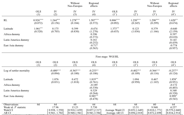
Our results are presented in Tables 4. Column (1) corresponds to Acemoglu et al. (2001)’s baseline model estimated by OLS. In column (2), the same model is estimated by IV. In column (3), we remove from the sample Neo-Europes (Australia, Canada, New Zealand, the United States). In column (4), we include regional dummy variables (Africa, East Asia, Latin America). Columns (1’)-(4’) provide the multiple imputation results. First-stage estimates and weak instrument diagnostics are also reported. The latter correspond to the first-stage F statistic14 and the Anderson-Rubin (AR) 95 % confidence interval, which is valid even
14Instruments are usually said to be strong (relevant) when the value of theF statistic is around 10 or higher
when the instrument is weakly correlated with the endogenous variable (Chernozhukov and Hansen, 2008). For the multiply-imputed regressions, we report the averages across 200 imputations of the lower and upper bounds of the Wald and AR confidence intervals.15
The estimates reported in columns (1)-(4) are very much in line with Acemoglu et al. (2001)’s findings. Whichever the robustness check used, governance has a causal and sub-stantial positive impact on income per capita and setter mortality is a relevant instrument. In column (4), the value of the first-stageF-statistic declines when we control for regional dummy variables, the AR confidence interval increases, but we still cannot reject the hypoth-esis that governance has no effect on income per capita.
Taking into account the uncertainty around the RL indicator makes little difference to the second-stage estimates but leads to larger standard errors, resulting in lower statistical significance. This result is the outcome of a weaker first-stage, as indicated by lower values of the first-stageF-statistic and larger Wald and AR confidence intervals.16
Overall, Acemoglu et al. (2001)’s findings are robust to accounting explicitly for the uncertainty of the RL indicator. This could have been expected, given that the estimation exploits the cross-sectional variation in governance quality and, as discussed earlier, some countries have very different and non-overlapping governance values. Nevertheless, with multiple imputation, estimation of the parameter of interest is less precise, reflecting that the RL indicator is measured with uncertainty.
15When using multiple imputation, calculation of the first-stage F statistic is straightforward. It simply
involves running the first-stage regression and testing the statistical significance of the IV. For other instrument diagnostics, it is not clear how their statistics should be combined and interpreted. Roodman (2012) reports the median values of the tests of overidentifying restrictionspvalues across 100 imputations and interpret them in the standard way. We report averages of the AR confidence intervals. However, in both cases, this is an ad hoc practice without strong theoretical foundations. It may nevertheless provide information about the validity of the IV.
16Note that these confidence intervals are different from those implied by the second-stage standard errors
Table 4: Long-run development and governance
Second stage: Log income per capita in 1995 ($ PPP)
With WGI uncertainty
Without Regional Without Regional
Neo-Europes effects Neo-Europes effects
OLS IV IV IV OLS IV IV IV
(1) (2) (3) (4) (1’) (2’) (3’) (4’)
RL 0.926∗∗∗ 1.244∗∗∗ 1.278∗∗∗ 1.587∗∗∗ 0.806∗∗∗ 1.250∗∗∗ 1.290∗∗∗ 1.620∗∗
(0.072) (0.156) (0.184) (0.372) (0.092) (0.245) (0.299) (0.674)
Latitude 1.061∗∗ 0.175 0.399 -0.474 1.373∗∗ 0.123 0.379 -0.640
(0.520) (0.703) (0.830) (1.270) (0.655) (1.036) (1.166) (2.159)
Africa dummy 0.396 0.397
(0.372) (0.618)
Latin America dummy 0.161 0.143
(0.252) (0.439)
East Asia dummy -0.717 -0.774
(0.563) (0.957)
First stage: WGI RL
OLS OLS OLS OLS OLS OLS OLS OLS
(1) (2) (3) (4) (1’) (2’) (3’) (4’)
Log of settler mortality -0.400∗∗∗ -0.365∗∗∗ -0.253∗∗ -0.402∗∗∗ -0.366∗∗∗ -0.257∗∗
(0.094) (0.100) (0.106) (0.109) (0.116) (0.124)
Latitude 1.076 0.472 1.819∗∗ 1.094 0.467 1.858∗
(0.831) (1.018) (0.761) (0.958) (1.165) (0.951)
Africa dummy -0.189 -0.172
(0.330) (0.403)
Latin America dummy 0.329 0.340
(0.264) (0.328)
East Asia dummy 0.985∗∗ 0.999∗
(0.478) (0.543)
Observations 64 64 60 64 64 64 60 64
Weak id.Fstatistic 17.96 13.23 5.730 13.51 9.948 4.257
Wald CI [ 0.938, 1.550] [0.918,1.639] [0.857,2.317] Average Wald CI [0.852,1.649] [0.810,1.771] [0.579,2.660]
1
3.4
Income inequality and democracy
3.4.1 Data and empirical approach
The impact of income inequality on democracy is a debated issue in the political literature. Boix (2003) argues that income equality promotes democracy whereas Acemoglu and Robin-son (2006) suggest that there is an inverse U-relationship between income inequality and democratisation. In opposition to these redistributivist theories, Ansell and Samuels (2010) develop a ‘contractarian’ approach, which predicts a positive impact of income inequality on democratisation. Their empirical results support such a hypothesis. We revisit this debate by using recently produced proxies for democracy and income inequality. Unlike the WGI, which come with a standard error which we used to do multiple imputations, these variables come with imputations already provided.
Our data on democracy come from the Unified Democracy Scores (UDS) database. Like the WGI, the UDS scores are the outcome of a sophisticated integration of many different rat-ings of democracy into a single measure. Scores range from -2.14 to 2.33, with a higher score indicating a more democratic political regime. Our data on income inequality correspond to the estimated Gini coefficients in the Standardized World Income Inequality Database (SWIID). The SWIID employs a custom missing-data algorithm to provide comparable es-timates of the Gini index of gross (pre-tax, pre-transfer) and net (post-tax, post-transfer) income inequality. Gini coefficients range from 0.16 to 0.71 with a higher coefficient indicat-ing greater inequality.17 In addition to a proxy, both UDS and SWIID provide imputed values of the variables. We directly use these values in our regressions.18
17The quality of the SWIID data has been questioned by Jenkins (2014) and others. However, much of this
criticism relates to an older version of the SWIID database. We are using the most recent update of this dataset (see Solt (forthcoming)) which attempts to address some of these criticisms.
18We only use 100 imputations because that is the maximum number of imputed values provided with SWIID.
We build on the specification of Acemoglu et al. (2008) in column 6 of their Table 3. More precisely, using annual observations, we estimate a fixed effects panel data model, but use a wider variety of explanatory variables than Acemoglu et al. (2008). The dependent variable is a measure of democracy which is regressed on five lags of each of democracy, income inequality, and log of income per capita. Similar to Acemoglu et al. (2008), the lags are included to account for inertia in the political process. Year dummies are included in all regressions. Our sample covers 142 countries over the period 1960-2010. Standard errors are clustered at the country level.
3.4.2 Empirical results
Our results are presented in Table 5. We report the cumulative dynamic multipliers (sum of the coefficients on the lags) associated with each variable as well as the long-run effect of inequality on democracy. Column (1) assumes a linear relationship between democracy and gross income inequality while column (2) assumes a quadratic relationship. In columns (3) and (4), gross income inequality is replaced by net income inequality. Columns (1)’-(4’) provide comparable multiple imputation results.
Table 5: Democracy and income inequality
Democracy (Unified Democracy Scores)
Fixed effects estimator With UDS/SWIID uncertainty
(1) (2) (3) (4) (1)’ (2)’ (3)’ (4)’
Cum. dynamic multiplier
Democracy 0.866*** 0.865*** 0.866*** 0.865*** 0.741*** 0.738*** 0.739*** 0.736***
(0.016) (0.016) (0.017) (0.017) (0.031) (0.031) (0.031) (0.031)
[0.018]*** [0.018]*** [0.018]*** [0.018]***
ln(GDPPC) -0.004 -0.002 -0.003 -0.000 -0.016 -0.012 -0.014 -0.006
(0.037) (0.039) (0.037) (0.039) (0.072) (0.073) (0.071) (0.073)
[0.038] [0.041] [0.037] [0.041]
Gross Gini 0.234** 0.671 0.290 1.313
(0.112) (0.904) (0.217) (1.513)
[0.121]* [0.918]
(Gross Gini)2 -0.499 -1.177
(1.051) (1.725)
[1.065]
Net Gini 0.328*** 0.728 0.505** 1.680
(0.117) (0.764) (0.239) (1.422)
[0.130]** [0.839]
(Net Gini)2 -0.523 -1.518
(0.996) (1.815)
[1.092]
Long-run effect
Gross Gini 1.747** 1.119
(0.868) (0.866)
[0.967]*
Net Gini 2.438*** 1.939**
(0.919) (0.964)
[1.041]**
Turning point 0.67 0.70 0.56 0.55
Observations 3139 3139 3139 3139 3139 3139 3139 3139
In column (4), we do not find evidence of a non-linear relationship between net income in-equality and democracy; the turning point is now higher than in column (2). Lastly, in all regressions, in line with the findings of Acemoglu et al. (2008), we find strong persistence of democracy over time as well as the absence of an impact of income per capita on democracy. Some changes in these findings occur when we use multiple imputation methods to take into account the uncertainty of both UDS scores and Gini coefficients. In column (1’), gross income inequality no longer has a statistically significant effect of democracy in the long-run. In column (3’), the cumulative dynamic multiplier of net income inequality is larger than the comparable number of column (3), but estimated less precisely and, thus, is less significant. Furthermore, the estimate of the long-run effect of income inequality on democracy is smaller in column (3’) than in column (3) because of a fall in the persistence of democracy. Finally, in columns (2’) and (4’), the turning points are smaller than in columns (2) and (4). They remain extremely large and the marginal effects of (gross or net) income inequality when using a quadratic function are never statistically significant at conventional levels.
Overall, we find some supportive evidence for a positive and linear relationship between income inequality and democracy, as put forward by Ansell and Samuels (2010). However, using multiple imputation, this result only holds for a measure of net income inequality, sug-gesting that authoritarian rulers can appease demands for democracy through a redistribution of income. Hence our results appear to be compatible with a contractarian approach in which redistribution still plays a role.
4
Conclusions
References
Acemoglu, Daron, Johnson, Simon, and Robinson, James A. (2001) ‘The Colonial Origins of Comparative Development: An Empirical Investigation’, American Economic Review, Vol. 91, pp. 1369–1401.
Acemoglu, Daron, Johnson, Simon, Robinson, James A., and Yared, Pierre (2008) ‘Income and Democracy’, American Economic Review, Vol. 98, pp. 808–842.
Acemoglu, Daron and Robinson, James A. (2006) Economic Origins of Dictatorships and
Democracy: New York: Cambridge University Press.
Alfaro, Laura, Kalemli-Ozcan, Sebnem, and Volosovych, Vadym (2008) ‘Why Doesn’t Cap-ital Flow from Rich to Poor Countries? An Empirical Investigation’, Review of Economics
and Statistics, Vol. 90, pp. 347–368.
Ansell, Ben and Samuels, David (2010) ‘Inequality and Democratization: A Contractarian Approach’, Comparative Political Studies, Vol. 43, pp. 1543–1574.
Azémar, Céline and Desbordes, Rodolphe (2013) ‘Has the Lucas Paradox Been Fully Ex-plained?’, Economics Letters, Vol. 121, pp. 183–187.
Baier, Scott L. and Bergstrand, Jeffrey H. (2009) ‘Bonus Vetus OLS: A Simple Method For Approximating International Trade-Cost Effects Using the Gravity Equation’, Journal of
International Economics, Vol. 77, pp. 77–85.
Berden, Koen, Bergstrand, Jeffrey H, and Etten, Eva (2014) ‘Governance and Globalisation’,
The World Economy, Vol. 37, pp. 353–386.
Binici, Mahir, Hutchison, Michael, and Schindler, Martin (2010) ‘Controlling Capital? Le-gal Restrictions and the Asset Composition of International Financial Flows’, Journal of
International Money and Finance, Vol. 29, pp. 666–684.
Boix, Carles (2003) Democracy and Redistribution: New York: Cambridge University Press.
Bolt, J. and van Zanden, J. L. (2013) ‘The First Update of the Maddison Project; Re-Estimating Growth Before 1820’, Maddison Project Working Paper 4.
Chernozhukov, Victor and Hansen, Christian (2008) ‘The Reduced Form: A Simple Ap-proach to Inference with Weak Instruments’, Economics Letters, Vol. 100, pp. 68–71.
Daude, Christian and Stein, Ernesto (2007) ‘The Quality of Institutions and Foreign Direct Investment’, Economics and Politics, Vol. 19, pp. 317–344.
Faria, Andre and Mauro, Paolo (2009) ‘Institutions and the External Capital Structure of Countries’, Journal of International Money and Finance, Vol. 28, pp. 367–391.
Head, Keith, Mayer, Thierry, and Ries, John (2010) ‘The Erosion of Colonial Trade Linkages After Independence’, Journal of International Economics, Vol. 81, pp. 1–14.
Høyland, Bjørn, Moene, Karl, and Willumsen, Fredrik (2012) ‘The Tyranny of International Index Rankings’, Journal of Development Economics, Vol. 97, pp. 1–14.
Jenkins, Stephen P. (2014) ‘World Income Inequality Databases: An assessment of WIID and SWIID’, IZA Discussion Paper, No. 8501.
Kaufmann, Daniel, Kraay, Aart, and Mastruzzi, Massimo (2009) ‘Governance Matters VIII: Aggregate and Individual Indicators, 1996-2008’, World Bank Policy Research Paper, No. 4978.
(2011) ‘The Worldwide Governance Indicators: Methodology and Analytical Is-sues’, Hague Journal on the Rule of Law, Vol. 3, pp. 220–246.
Kaufmann, Daniel, Kraay, Aart, and Zoido-Lobaton, Pablo (1999) ‘Aggregating Governance Indicators’, World Bank Working Paper, No. 2195.
Lane, Philip R. and Milesi-Ferretti, Gian Maria (2007) ‘The External Wealth of Nations Mark II: Revised and Extended Estimates of Foreign Assets and Liabilities, 1970-2004’, Journal
of International Economics, Vol. 73, pp. 223–250.
Milner, Helen V and Mukherjee, Bumba (2009) ‘Democratization and Economic Globaliza-tion’, Annual Review of Political Science, Vol. 12, pp. 163–181.
Pemstein, Daniel, Meserve, Stephen A, and Melton, James (2010) ‘Democratic Compromise: A Latent Variable Analysis of Ten Measures of Regime Type’, Political Analysis, Vol. 18, pp. 426–449.
Rodrik, Dani, Subramanian, Arvind, and Trebbi, Arvind (2004) ‘Institutions Rule: The Pri-macy of Institutions Over Geography and Integration in Economic Development’, Journal
of Economic Growth, Vol. 9, pp. 131–165.
Roodman, David (2012) ‘Doubts About the Evidence That Foreign Aid For Health is Dis-placed Into Non-Health Uses’, The Lancet, Vol. 380, pp. 972–973.
Rubin, Donald B (1996) ‘Multiple Imputation After 18+ years’, Journal of the American
Solt, Frederick (forthcoming) ‘The Standardized World Income Inequality Database’, Social
Science Quarterly.
Staiger, Douglas and Stock, James H. (1997) ‘Instrumental Variables Regression with Weak Instruments’, Econometrica, Vol. 65, pp. 557–586.
Standaert, Samuel (forthcoming) ‘Divining the Level of Corruption: A Bayesian State-Space Approach’, Journal of Comparative Economics.
Treisman, Daniel (2007) ‘What Have We Learned About the Causes of Corruption From Ten Years of Cross-National Empirical Research?’, Annual Review of Political Science, Vol. 10, pp. 211–244.
Appendices
A
Description of variables
The variables used in the empirical applications are described in Table 6.
B
Stata pseudo-code
We present below how the uncertainty around the WGI estimate Voice and Accountability can be taken into account in Stata, using multiple imputation.
label var wgivae “Value of the estimate”
label var wgivas “Standard error of the estimate”
qui forval i=1/200 {
gen diff=rnormal()
gen imput‘i’= diff*wgivas+wgivae
drop diff
}
gen MIwgiva=.
mi import wide,imputed(MIwgiva=imput1-imput200) clear
Table 6: Description of variables
Application Variable Description Source
WGI Worldwide Governance Indicators (WGI) Six Worldwide Governance Indicators (VA, PS, GE, RQ, RL, CC) WGI project
1996-2010 (www.govindicators.org)
Capital flows Capital inflows (debt or equity) -min(∆assets,0)+max(∆liabilities, 0); per capita, in US $ Lane and Milesi-Ferretti (2007)
71 countries Capital outflows (debt or equity) max(∆assets,0)-min(∆liabilities, 0); per capita, in US $ Lane and Milesi-Ferretti (2007)
1998-2005 Capital in/out-flow control Index of financial openness (0-1, from least to most regulated) Schindler (2009)
WGI (1998, 2000, 2002-2005) Population Total population World Development Indicators
GDP per cap GDP per capita, in constant 2000 US $ World Development Indicators
(Fuel, Metals, Ore)/ Exports Sum of the fuel, metals and ore exports divided by total exports World Development Indicators
Trade openness (Exports+Imports)/GDP World Development Indicators
Private credit/GDP Private credit by deposit money banks and other financial institutions to GDP Beck et al. (2009)
STMK CAP/GDP Value of listed shares to GDP Beck et al. (2009)
International trade GDP GDP, in constant 2000 US $ World Development Indicators
180 countries GDPPC GDP per capita, in constant 2000 US $ World Development Indicators
1998-2004 Bilateral trade flows Exports from countryito countryj Head et al. (2010)
WGI (1998, 2000, 2002-2004) Distance Population-weighted bilateral distance (km) Head et al. (2010)
Contiguity 1 if two countries share a common border Head et al. (2010)
Common language 1 if a language is spoken by at least 9% of the population in both countries Head et al. (2010)
Colonial links 1 for pair even in colonial relationships Head et al. (2010)
Multilateral resistance (MR) terms Calculated following Baier and Bergstrand (2009)
Income levels Log of income per capita Income per capita in 1995 ($ PPP basis) Acemoglu et al. (2001)
64 countries (http://economics.mit.edu/faculty/acemoglu/data/ajr2001 )
1995 Latitude Absolute value of the latitude of the country Acemoglu et al. (2001)
WGI RL only (1996) Settler mortality Estimated settlers’ mortality rate Acemoglu et al. (2001)
Regional dummy variables Regional indicators for Africa, East-Asia, Latin America and the Caribbean Rodrik et al. (2004)
Democracy and Income inequality Democracy Unified Democracy Scores Pemstein et al. (2010)
142 countries (http://www.unified-democracy-scores.org/)
1960-2010 Income inequality Gross and net (post-tax, post-transfer) income inequality Solt (forthcoming); version 5, updated October 2014
(http://myweb.uiowa.edu/fsolt/swiid/swiid.html)
GDPPC GDP per capita, in PPP 1990 US$ Bolt and van Zanden (2013)
2