Pattern recognition techniques applied to rust classification in steel structures

(1)

City, University of London Institutional Repository

Citation

:

Zhang, Yun (2012). Pattern recognition techniques applied to rust classification in steel structures. (Unpublished Masters thesis, City University London)

This is the unspecified version of the paper.

This version of the publication may differ from the final published

version.

Permanent repository link: http://openaccess.city.ac.uk/3007/

Link to published version

:

Copyright and reuse:

City Research Online aims to make research

outputs of City, University of London available to a wider audience.

Copyright and Moral Rights remain with the author(s) and/or copyright

holders. URLs from City Research Online may be freely distributed and

linked to.

City Research Online: http://openaccess.city.ac.uk/ [email protected]

(2)

PATTERN RECOGNITION TECHNIQUES APPLIED TO RUST

CLASSIFICATION IN STEEL SURFACES

Yun Zhang

Master of Philosophy

City University

Department of Computing

(3)

LIST OF FIGURES

Number Page

Figure 1.1 Evaluation process for a protective coating system [Pietsch, Kaiser 02] 14

Figure 1.2 International standard of rust grades A, B, C and D ... 16

Figure 1.3 Diagrams representing rust grades and the correspond area percentage 16 Figure 1.4 Mechanical cleaning method [Momber 03] ... 18

Figure 1.5 The working environment to apply the hydro-blasting preparation method ... 19

Figure 1.6 Previous Research - System structure to classify six classes [Ünsalan 95] 24 Figure 1.7 Previous Research - System structure of the binary classification [Ünsalan 95] ... 24

Figure 1.8 Previous Research - Classification result for GLCM [Ünsalan 95] 24 Figure 2.1 Example of image regions corresponding to (a) class A and (b) class B. 31 Figure 2.2 Plot of the mean value versus the standard deviation for a number of different images originating from class A (o) and class B (+) ... 31

Figure 2.3 The basic stages involved in the design of a classification system . 33 Figure 2.4 The flow chart of the process of designing a learning machine for pattern recognition ... 35

Figure 2.5 Multiple-input Neuron ... 48

Figure 2.6 Trajectory with and without Momentum ... 52

Figure 2.7 Artificial Texture ... 58

Figure 2.8 - Source Image and Co-occurrence Matrix of the source image ... 62

Figure 3.1 Image size optimization ... 70

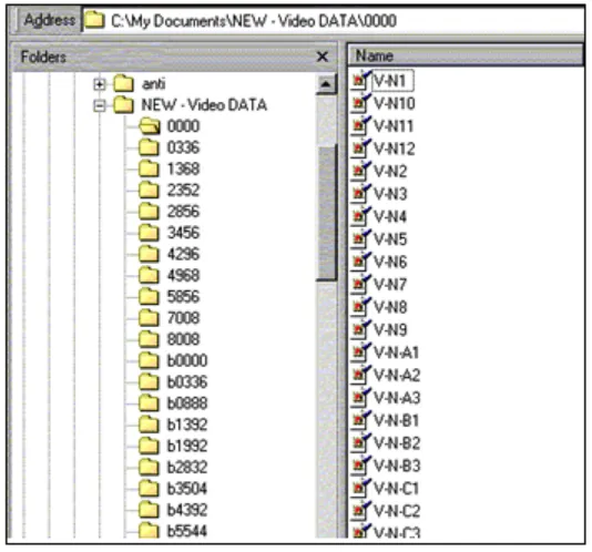
Figure 3.2 The structures in Video Library ... 71

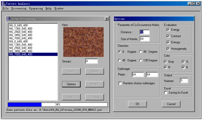
Figure 3.3 Visual library optimization user interface ... 74

Figure 3.4 Feature extraction user interface ... 74

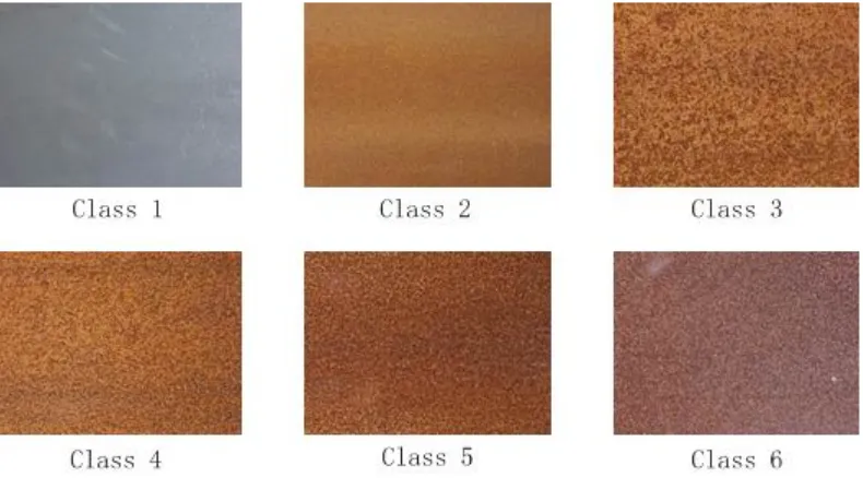
Figure 3.5 One set of rust images which contains six classes ... 76

Figure 3.6 Combinations of different feature sets ... 77

(6)

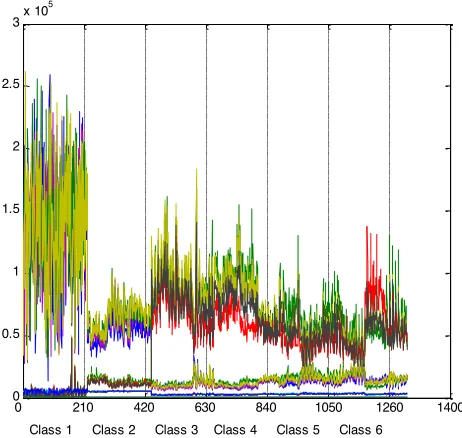
Figure 3.8 Co-Occurrence matrices of the six classes represented in all colour channels

- Colour Channel View ... 79

Figure 3.9 Co-Occurrence matrices of the six classes represented in all colour channels - 3D view ... 80

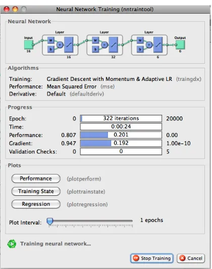
Figure 3.10 The training progress of a neural network which is used to classify six classes ... 83

Figure 3.11 The discriminant analysis ... 84

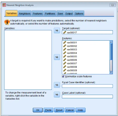
Figure 3.12 Nearest neighbour analysis ... 84

Figure 3.13 Overall structure of the classification system structure ... 86

Figure 4.1 Training performance and error histogram: the binary classification of the class one ... 97

Figure 4.2 Training performance and error histogram: the binary classification of the class two ... 98

Figure 4.3 Training performance and error histogram: the binary classification of the class three ... 99

Figure 4.4 Training performance and error histogram: the binary classification of the class four ... 100

Figure 4.5 Training performance and error histogram: the binary classification of the class five ... 101

Figure 4.6 Training performance and error histogram: the binary classification of the class six ... 102

Figure 4.7 Training performance and error histogram: the classification of three classes ... 103

Figure 4.8 Training performance and error histogram: the classification of four classes ... 104

Figure 4.9 Training performance and error histogram: the classification of five classes ... 105

Figure 4.10 Training performance and error histogram: the classification of six classes ... 106

Figure 4.11 Canonical discriminate functions of three classes ... 111

Figure 4.12 Canonical discriminate functions of four classes ... 112

Figure 4.13 Canonical discriminate functions of five classes ... 113

(7)

Figure 4.15 KNN feature space – classification of three classes ... 119

Figure 4.16 KNN feature space – classification of four classes ... 120

Figure 4.17 KNN feature space – classification of five classes ... 121

(8)

LIST OF TABLES

Number Page

Table 4.1 ADALINE - Evaluate results: the binary classification of the class one 89

Table 4.2 ADALINE - Evaluate results: the binary classification of the class two 89

Table 4.3 ADALINE - Evaluate results: the binary classification of the class three 89

Table 4.4 ADALINE - Evaluate results: the binary classification of the class four 90

Table 4.5 ADALINE - Evaluate results: the binary classification of the class five 90

Table 4.6 ADALINE - Evaluate results: the binary classification of the class six 91

Table 4.7 LVQ - Evaluate results: the binary classification of the class one ... 92

Table 4.8 LVQ - Evaluate results: the binary classification of the class two ... 92

Table 4.9 LVQ - Evaluate results: the binary classification of the class three . 92 Table 4.10 LVQ - Evaluate results: the binary classification of the class four 93 Table 4.11 LVQ - Evaluate results: the binary classification of the class five . 93 Table 4.12 LVQ - Evaluate results: the binary classification of the class six .. 94

Table 4.13 LVQ - Evaluate results: the classification of three classes ... 94

Table 4.14 LVQ - Evaluate results: the classification of four classes ... 95

Table 4.15 LVQ - Evaluate results: the classification of five classes ... 96

Table 4.16 LVQ - Evaluate results: the classification of six classes ... 96

Table 4.17 BP - Evaluate results: the binary classification of the class one .... 98

Table 4.18 BP - Evaluate results: the binary classification of the class two .... 99

Table 4.19 BP - Evaluate results: the binary classification of the class three .. 99

Table 4.20 BP - Evaluate results: the binary classification of the class four 100 Table 4.21 BP - Evaluate results: the binary classification of the class five . 101 Table 4.22 BP Evaluate results: the binary classification of the class six ... 102

Table 4.23 BP - Evaluate results: the classification of three classes ... 103

Table 4.24 BP - Evaluate results: the classification of four classes ... 104

Table 4.25 BP - Evaluate results: the classification of five classes ... 105

Table 4.26 BP - Evaluate results: the classification of six classes ... 107

(9)

Table 4.28 Discriminant analysis cross-validated result: Binary classification of the

class two ... 108

Table 4.29 Discriminant analysis cross-validated result: Binary classification of the class three ... 109

Table 4.30 Discriminant analysis cross-validated result: Binary classification of the class four ... 109

Table 4.31 Discriminant analysis cross-validated result: Binary classification of the class five ... 110

Table 4.32 Discriminant analysis cross-validated result: Binary classification of the class six ... 110

Table 4.33 Discriminant analysis cross-validated result: Classification of three classes ... 111

Table 4.34 Discriminant analysis cross-validated result: Classification of four classes ... 112

Table 4.35 Discriminant analysis cross-validated result: Classification of five classes ... 114

Table 4.36 Discriminant analysis cross-validated result: Classification of six classes 115 Table 4.37 KNN result: Binary classification of the class one ... 116

Table 4.38 KNN result: Binary classification of the class two ... 116

Table 4.39 KNN result: Binary classification of the class three ... 117

Table 4.40 KNN result: Binary classification of the class four ... 117

Table 4.41 KNN result: Binary classification of the class five ... 118

Table 4.42 KNN result: Binary classification of the class six ... 118

Table 4.43 KNN result: Classification of three classes ... 119

Table 4.44 KNN result: Classification of four classes ... 121

Table 4.45 KNN result: Classification of five classes ... 122

Table 4.46 KNN result: Classification of six classes ... 123

Table 4.47 The performances of the BP trained by different feature sets ... 126

(10)

ACKNOWLEDGMENTS

I would like to thank my wife for her help, an extraordinary patience, encourage and

support during the research that led to completion of this thesis.

I am most grateful to my supervisors Dr. Andrew Tuson, Dr. Peter Smith and Dr. Geoff

Dowling for their support, advice and attention to details. This thesis would not exist

without their help.

Thanks to for the Automated Inspection and Maintenance of Steel Structures (AIMS)

project team who supports me the entire steel surface visual library.

I thank all at the Department of Computing for providing a friendly environment to

work in.

Also thanks to all the other people, not mentioned here, who have supported and helped

(11)

University Librarian is allowed to copy the thesis in whole or in part without further

reference to the author. This permission covers only single copies made for study

(12)

ABSTRACT

The life and performance of steel structure depends directly upon the steel surface

preparation. The restoration of steel structure such as steel bridges, ships and storage

tanks is due mainly to the use of manual surface inspection methods accompanied by

surface preparation technologies. It requires a long project duration, high costs and

hazardous practices for both worker and environment to complete surface restoration.

The developments of surface preparation technologies make it essential to develop

technologies that allows patch restore of corrode steel structure in practice.

This thesis addresses the problem of classification of rust steel surfaces. Various Pattern

recognition methods are studied for classifying less subjective steel surfaces from a

time corrosion perspective. Our primary contribution is: with appropriate features from

the steel surfaces, artificial neural network pattern recognition methods have the

abilities to classify the less subjective rust steel surfaces reliably and be suitable for

automation. The results provide important information about the classification methods

for rust steel surface analysis.

(13)

ABBREVIATIONS AND TERMS

ADALINE Adaptive Linear Neuron network

ALC Adaptive Lineal Combiner

BP Back-Propagation network

ER Electrical Resistance

GLCM Gray Level Co-occurrence Matrices

KNN K-Nearest Neighbour method

LMS Least Mean Squares algorithm

LPR Linear Polarization techniques

LVQ Learning Vector Quantization

NDT Non Destructive Testing

MANOVA Multivariate analysis of variance

(14)

Chapter 1 - Introduction and Overview

1.1 Industry Background

Steel is the most commonly used metal material in the modern life. The reason to

choose steel among all metals is the strength and ease of production of steel.

However, steel corrode in many media including most outdoor atmospheres. The

serious consequences of the steel corrosion process have become a problem of

worldwide significance [Roberge 06]. Protective coatings are probably the most

widely used products for steel corrosion control. They are used to provide long-term

protection of steel structure under a broad range of corrosive condition, extending

from atmospheric exposure to the most demanding condition.

1.1.1 Steel Surface Preparation Definition

The life of a coating of steel structure depends as much on the degree of surface

preparation as on the subsequent coating system. Surface preparation is defined in IS0

12944-4 as ‘any method of preparing a surface for coating’. It is an important part of

any steel corrosion protection strategy [Momber 03].

The primary functions of steel surface preparation are to clean the steel surface of

material that will induce premature failure of the coating system and provide a surface

(15)

The ISO 8502 states that the performance of protective coatings of paint and related

products applied to steel is significantly affected by the state of the steel surface

immediately prior to painting. The principal factors that are known to influence the

performance are:

• The presence of rust and mill scale;

• The presence of surface contaminants, including salts, dust, oil and greases;

• The surface profile, which includes primary, roughness and waviness profiles.

The major factors for the selection of a corrosion protection system [Pietsch, Kaiser 02]

are shown in the Figure 1.1.

Evaluation Construction

material

Surface preparation

degree

Category of

corrosivity Lifetime Binder primer Binder top coat Local demands Selection of binder

Protective coating system

Figure 1.1 Evaluation process for a protective coating system [Pietsch, Kaiser 02]

1.1.2 Steel Surface Preparation Standards

(16)

extended the Swedish SIS 0559900, transformed into ISO 8501-1:1988 international

standard on rust. It defines rust grades and preparation grades of uncoated steel

substrates and steel substrates after overall removal of pervious coatings

The rust grades of uncoated steel surface are classified as A, B, C and D from

minimum to maximum by a human expert. The descriptions about them are shown

below and the images of rust grades show in the Figure 1.2.

• Rust grade A: Steel surface largely covered with adhering mill scale but litter,

if any, rust – This would correspond to a hot-rolled steel surface newly made.

• Rust grade B: Steel surface which has begun to rust and from which the mill

scale has begun to flake – This would correspond to a hot-rolled steel surface

exposed to wind and weather without protection into a moderately corrosive

atmosphere, for two or three months.

• Rust grade C: Steel surface on which the mill scale has rusted away or from

which it can be scraped, but with slight pitting visible under normal vision –

This would correspond to a steel surface exposed to wind and weather without

protection, into a moderately corrosive atmosphere, for about a year.

• Rust grade D: Steel surface on which the mill scale has rusted away and on

which general pitting is visible under normal vision – This would correspond

to a steel surface that was exposed to wind and weather, without protection,

(17)

[image:17.595.196.398.387.611.2]

Figure 1.2 International standard of rust grades A, B, C and D

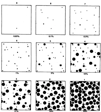
The Figure 1.3 shows a series of 1.5 inch squares with black dots representing various

area percentages. These diagrams are not proposed to reproduce the appearance of

actual rust patterns but simply to serve as a guide for judging the percentage of

surface covered by rust or rust blisters.

Figure 1.3 Diagrams representing rust grades and the correspond area percentage

1.1.3 Procedure for Visual Assessment of Steel Substrates

(18)

commonly used to assess the steel substrates. This procedure requires either in good

diffuse daylight or in equivalent artificial illumination to examine the steel surface

and compare it with each of the photographs of the standard rust grades, using normal

vision. Place the appropriate photograph close to, and in the plane of, the steel surface

to be assessed. For rust grades, record the assessment as the worst grade that is

evident.

1.1.4 Steel Surface Preparation Methods

Definition and subdivision of steel preparation methods are listed in ISO 12944-4

(1998). Basically, the following three principal surface preparation methods can be

distinguished:

• Water, solvent and chemical cleaning that includes water cleaning, steam

cleaning, emulsion cleaning etc.

• Mechanical cleaning method that includes hand-held tool cleaning, power-tool

cleaning, blast cleaning and water blast cleaning.

• Flame cleaning

(19)

Mechanical Cleaning methods

Hand-held tool

cleaning Power-tool cleaning Blast-cleaning

Water blast-cleaning (Hydro-blasting)

Figure 1.4 Mechanical cleaning method [Momber 03]

The hydro-blasting method is the most effective mechanical cleaning method by far.

Hydro-blasting is a technique for cleaning surfaces, which relies entirely on the

energy of water striking a surface to achieve its cleaning effect. The tool of any

hydro-blasting application is a high-speed water jet. Although the speed of the jet is

its fundamental physical property, the pressure generated by the pump unit that

produces the jet is the most important evaluation parameter in practice. Water jet

applications can be distinguished according to the level of the applied operational

pressure as follows [Momber 03]:

a) Pressure cleaning: the use of pressurised water, with or without the addition of

other liquids or solid particles, to remove unwanted matter from various

surfaces, and where the pump pressure is below 340 bar.

b) High-pressure water cleaning: the use of high-pressure water, with or without

(20)

from various surface, and where the pump pressure is between 340 and 2000

bar.

c) Ultra high-pressure water cleaning: the use of pressurised water, with or

without the addition of other liquids or solid particles, to remove unwanted

matter from various surfaces, and where the pump pressure exceeds 2000 bar.

The Figure 1.5 shows a typical working environment to apply hydro blasting method.

Figure 1.5 The working environment to apply the hydro-blasting preparation method

1.2 Problem Statement

1.2.1 Disadvantages of Visual Assessment of Steel Substrates

Firstly, the human inspection is commonly used to assess the steel substrates (see

section 1.1.3). The human experts normally assess rust conditions by surveying a steel

(21)

used in this evaluation process are often subjective in nature and are based on the

experiences of the evaluator. Currently, photographic standards are used for

classification of the level of corrosion of coated steel surfaces, as well as, to assess the

levels of cleanliness achieved by the established surface preparation methods. The

visual standard may difficult to use due to differing appearances of steel, hue and

lighting effects. Because of this, the possibility exists that an error may enter the

evaluation process that, due to the length of the maintenance cycle, could result in the

collapse of the structure before it can be repaired.

Secondly, destructive testing methods have to be applied to support coating condition

in some cases.

Final, Only spot inspection is practical.

1.2.2 The Hazards of Steel Surface Preparation

As the most common and effective method (see section 1.1.4), the blasting cleaning

operation is an activity with significant inherent hazards. If work task are approached

inappropriately, significant risks with the potential of serious injury, including fatality

are possible. The ISO 12944-4 stats the following for surface preparation in general:

‘All relevant health and safety regulations shall be observed.’ Hydro blasting has a

(22)

of danger to hydro-blasting operations include the following:

• Reactive forces generated by the exiting water jets.

• Cutting capability of the high-speed jets;

• Hose movements (especially during switch-on of the pump).

• Working in areas of electric devices;

• Uncontrolled escape of pressurised water.

• Damaged parts being under pressure.

• Dust and aerosol formation.

• Sound emitted from equipment and water jet.

• Impact from rebounding debris from the jet impact point.

1.2.3 Conclusions

To overcome the problems listed in section 1.2.1 and 1.2.2, it is essential to develop a

robotic system to automatically perform the inspection and cleaning operation. The

key design criterion for a robotic system is the rust detection and measurement

method. Currently, several methods for rust detection and measurement have been

research. There methods fall into two categories; they are non-direct (non-intrusive)

and direct (intrusive) techniques. Direct techniques such as Corrosion Coupons,

Electrical Resistance (ER) and the Linear-polarization techniques (LPR) are small

(23)

large scale and non-contacting method, the visual inspection method seems to be

more suitable for the robotic system.

1.3 Previous Research

1.3.1 Material Surface Classification

There are some relative researches related with material surface classification have

been done. Some typical researches are listed below:

• Reniers [[Reniers 08] has present a method to be sued to detect convex ridges

on voxel surface extracted from 3D scans.

• Lepistö [Lepistö 03] has introduced a rock texture classification method,

which is based upon textural and spectral features of the rock and the textural

features are calculated from the co-occurrence matrix. Two types of rock

textures are tested, and the experimental results show that the proposed

features are able to classify rock textures.

• Sharma [Sharma 00] has worked on Meastex images (A number of image sets

which contain examples of artificial and natural textures. Each image has a

size of 512×512 pixels and is distributed in raw PGM format) to evaluate the

textures methods for image analysis, in which four group images of asphalt,

concrete, grass and rock are tested.

• Bruno [Bruno 99] has applied the different statistical and spectral method to

(24)

• Don and Fu [Don 84] have inspected metal surface by the roughness of the

surface.

1.3.2 Steel Surface Classification

The fundamental research of steel surface classification has been done by Ünsalan and

Ercil [Ünsalan 95, Ünsalan 98 and Ünsalan 99]. They have considered the problem

of studying pattern recognition techniques for analysing textured surface and applied

the results to the classification of steel surface. In their research, various texture

analysis methods had been applied to extract features from steel surfaces. All the

features were optimized by feature selection and extraction algorithms and then fed

into a classifier.

They have used a K-Nearest Neighbour classifier (KNN) to classify six different steel

surface types (grades A, B, C of both rust grades and sandblasted forms, see section

1.1.2), and a Combining classifier for the binary classification. The system structures

are given in Figure 1.6 and Figure 1.7. Figure 1.8 shows the classification results for

(25)

Figure 1.6 Previous Research - System structure to classify six classes [Ünsalan 95]

Figure 1.7 Previous Research - System structure of the binary classification [Ünsalan

95]

Figure 1.8 Previous Research - Classification result for GLCM [Ünsalan 95]

(26)

from GLCM (Gray Level Co-occurrence Matrices Method) and MRF (Markov

Random Fields Method) can be used by a KNN classifier to discriminate the six types

(uncoated and prepared rust grades A, B and C) of steel surface with very high

accuracy.

1.4 Objectives

The previous research has made some results, but there are still some areas need to be

researched further:

• The statistical pattern recognition method (KNN classifier) is the only

approach applied in the previous research to classify six types of steel surface.

Two kind of artificial neural networks, Kohonen’s learning vector quantization

(LVQ) and ADALINE have only been applied to make the binary decision.

The artificial neural networks have been commonly used in pattern recognition

as a natural pattern classifier and cluster. The artificial neural network can

approximate every classification function as closely as required in theory. A

question has been raised is “can an artificial neural network solve the same

problem of non-destructive steel surface classification or even perform

(27)

• All previous researches are focused on the uncoated and prepared rust grade A,

B and C. Is there any possibility to discriminate the continuous and less

subjective rust grades

In this thesis, the problem of classification of steel surfaces is considered. This

research therefore will focus on the above two problems to use artificial neural

network and statistical pattern recognition techniques to classify continuous and less

subjective grades of rust rather than simply A to C grades.

1.5 Outline of the Thesis

Chapter 2 provides an overview of texture analysis methods and pattern recognition

methods which have been applied for this research.

Chapter 3 explains how to obtain features from the steel surface. A visual library

which contains 500 pictures representing rust between 0 to 8000 hours has been

adopted. Six different steel surface types are selected form this visual library and the

Co-occurrence Matrices method is applied as the feature extraction algorithms. The

classification approaches are also provided in this chapter. Various artificial neural

network and statistic pattern recognition methods are examined.

(28)

Chapter 2 - Literature Review

This chapter explains some key concepts for pattern recognition techniques as well as

and texture analysis methods

This research will implement some of the pattern recognition techniques and texture

analysis methods in order to solve the rust image classification problem.

Texture analysis is one possible method to detect features in images. As a well-know

statistical method it measures second-order texture characteristics of an image, the

Co-occurrence matrix method is introduced as the main method for feature extraction.

There are three major approaches to design a pattern recognition system. However,

we only focus on two approaches – statistical pattern recognition and artificial neural

network pattern recognition.

This chapter also explains various pattern recognition methods practised within this

research along with their advantages and disadvantages, which are:

1) The Discriminant analysis and K-Nearest Neighbour analysis are introduced

(29)

2) ADALINE neural network, LVQ (learning and vector quantization) network

and Multilayer feed-forward neural network are introduced as artificial pattern

recognition methods.

2.1 Introduction of Pattern Recognition

The definition of pattern is - “A pattern is essentially an arrangement or an ordering in

which some organization of underlying structure can be said to exist” [Pandya 96].

Pattern recognition is the scientific discipline that has a goal to classify objects into a

number of categories or classes. These objects can be images or signal waveforms or

any type of measurements that need to be classified by different applications.

Pattern recognition has a long history, but it was mostly the output of theoretical

research in the area of statistics before the 1960s. However, the demands for

practical applications of pattern recognition are increased by the advent of computers,

and pattern recognition becomes an important field of computer science and electrical

engineering that studies the operation and design of systems to recognize patterns in

data. Important tasks that have been tackled are image analysis, character recognition,

speech analysis, man and machine diagnostics, person identification and industrial

inspection etc. Pattern recognition also is an integral part in most machine intelligence

systems which built for decision making. Pattern recognition is very important in the

(30)

obtain descriptions of what is imaged [Theodoridis 06].

There are two paradigms for pattern recognition, classification and cluster analysis.

Classification pattern recognition is also called supervised pattern recognition – there

is a predefined set of classes of patterns and the tasks are to classify a future pattern as

one of these classes. The classifier is designed by exploiting this a priori known

information. In cluster analysis (also known as unsupervised pattern recognition),

the aim is to seek groups of patterns, where a pattern needs to be assigned to a so far

unknown class of patterns.

Pattern recognition aims to map input feature space to the output class space, and is

concerned with making decision from complex patterns of information [Ripley 96]

such that:

a) Each input vector is mapped to one and only one class. This is to say each

sample vector in the input space will be assigned to one class only.

b) Many input vectors map to one class. The classification algorithm categorizes

the input space.

c) The class space is constructed by the information that extracted from the

(31)

algorithms are the constructions of the class space. Each classifier has its own

characteristic rules to construct the class space.

d) All the vectors from the input space that have not been used in training are

also mapped to one class in the output class space. This is the generalization

principle of the classification algorithm. The performances of the classifiers

are measured by their correct classification rates of test sample set [Ünsalan

98].

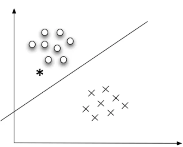
To give an example for the classification: Figure 2.1 shows two images, each having a

distinct region inside it. To distinct these two regions, the measurable quantities need

to be identified. Figure 2.2 shows a plot of the mean value of the intensity in each

(32)

[image:32.595.111.486.78.282.2]

Figure 2.1 Example of image regions corresponding to (a) class A and (b) class B.

Figure 2.2 Plot of the mean value versus the standard deviation for a number of

[image:32.595.140.446.415.660.2]

(33)

Each point corresponds to a different image from the available database. It shows that

class A patterns tend to spread in a different area from class B patterns. The straight

line seems to separate the two classes. If a new image which is not identified to

neither class is provided, we can measure the mean intensity and standard deviation in

the region of interest of the new image and plot the corresponding point. This is

shown by the asterisk (*) in Figure 2.2. Then it is more reasonable to assume that the

unknown pattern is more likely to belong to class A than class B. The mean value and

the standard deviation in this case, are known as features. In the more general case l

features xi i=1,2,...,l , are used and they form the feature vector

Where T denotes transposition and each of the feature vectors identifies uniquely a

single pattern (object).

The straight line in Figure 2.2 is called the decision line, and it establishes the

classifier whose role is to divide the feature space into regions that correspond to

either class A or class B.

Figure 2.3 shows the different stages followed for the design of a classification system.

These stages are interrelated, and depending on the results, one may go back to

(34)

Sensor _generationFeature _selectionFeature Classifier _design _evaluationSystem Patterns

Figure 2.3 The basic stages involved in the design of a classification system

The major approaches to design a pattern recognition system are:

• Statistical pattern recognition.

• Syntactic or structural pattern recognition.

• Artificial neural network (ANN) pattern recognition.

In statistical pattern recognition, the problem of pattern classification is described as a

statistical decision problem and it learns all information from examples. Statistical

pattern recognition is a mature theories and a number of commercial recognition

systems have been designed.

In structural pattern recognition, the properties of information about the class are used

to structure the problem. In syntactic pattern recognition, the information is provided

by the grammar of a formal language. The patterns are represented in a hierarchical

(35)

In artificial neural network pattern recognition, neural networks are implemented as a

class of mathematical algorithms and provide solutions to a number of specific

problems. Artificial neural network techniques are strongly related to corresponding

statistical method. More details about artificial neural network will be introduced

later.

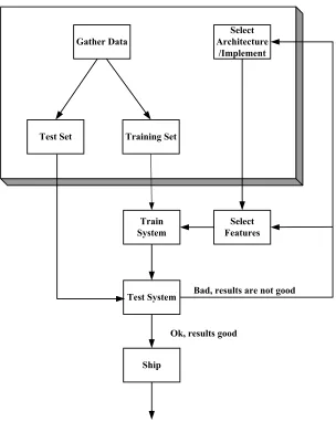
Figure 2.4 shows the steps involved in the design of a typical pattern recognition

(36)

Gather Data

Select Architecture

/Implement

Test Set Training Set

Train System

Select Features

Test System

Ship

Bad, results are not good

[image:36.595.141.445.69.451.2]

Ok, results good

Figure 2.4 The flow chart of the process of designing a learning machine for pattern

recognition

2.2 Statistical pattern recognition methods

2.2.1 Discriminant Analysis

There are many different ways to represent pattern classifiers. One of the most useful

is in term of a set of discriminant functions. Theory behind the discriminant function

(37)

A discriminant is a multivariate test to detect relationships between several dependent

variables. It is applied to determine which features discriminate between a numbers of

groups. A discriminant function is a linear combination of dependent variables and

can be described as a set of multiple regression equations. The standard expression of

multiple regression is shown below.

i n nX X

X β β ε

β β

γ = ₀ + ₁ ₁+ ₂ ₂+...+ +

Where, γ is the outcome variable, β_m(m∈[1,n])is the coefficient of _mth_predictor.

i

ε is the difference between the predicted and the observed value of γ for the _ith

subject.

The β values in the discriminant function are weights which describe the

contribution of each dependent variable to the variate and are obtained from the

eigenvectors of the product of the model sum of squares and cross-product (SSCP)

matrix (H) and the inverse of residual SSCP matrix (E-1). Matrix H contains the model

sums of squares for each dependent variable and the model cross-product between the

two dependent variables. Similarly, matrix E-1_{contains the residual sums of squares}

for each dependent variable and the residual cross-product between the two dependent

variables [Field 00].

Before giving an introduction to the product of the model SSCP matrix (H) and the

(38)

a) Model Sum of Squares (SSM): shows how much of the total variation can be

explained by the fact that different data points come from different groups, it

is obtained by SSM =

∑

ni(xi−xgrand)

2

.

Where x_i is the mean of each group. x_grand is the grand mean and n_i is the

number of scores of each group.

b) Residual Sum of Squares (SSR): shows how much of the variation cannot be

explained, =

∑

₍ − ₎2

i i

R x x

SS .

Where x_i is each score in a group and x_i is the mean of the group from

which x_i came.

c) Cross-product (CP): The difference between the scores and the mean in one

group multiplied by the difference between the scores and the mean in the

other groups. Two cross-products should be calculated, they are:

The model cross-product (CPM) – show how the relationship between the

dependent variable is influenced by experimental manipulation:

[

]

∑

− −

= ( group(group1) grand(group1))...( group(groupm) grand(groupm))

M n x X x X

CP

where xgroup(groupm) is the mean of each group, Xgrand(groupm) is the grand

(39)

The residual cross-product (CPR) – show how the relationship between the

dependent variables is affected by individual differences.

CPR =

∑

(xi₍group₁₎ −Xgroup(group1))...(xi₍group_m₎ −Xgroup(groupm))

where ₍ ₎

m group i

x is each score in group m, Xgroup(groupm) is the group mean.

Now, the definitions of the model SSCP matrix (H) and the residual SSCP matrix (E)

can be defined as:

⎥ ⎥ ⎥ ⎥ ⎥ ⎦ ⎤ ⎢ ⎢ ⎢ ⎢ ⎢ ⎣ ⎡ = ) ( ) ( ) ( ... ... ... ... ... ... ... 2 1 m group M M M M group M M M M group M SS CP CP CP SS CP CP CP SS H

H represents both the unsystematic variation that exists for each dependent variable

and the co-dependence between the dependent variables that is duo to chance factor

alone. ⎥ ⎥ ⎥ ⎥ ⎥ ⎦ ⎤ ⎢ ⎢ ⎢ ⎢ ⎢ ⎣ ⎡ = ) ( ) ( ) ( ... ... ... ... ... ... ... 2 1 m group R R R R group R R R R group R SS CP CP CP SS CP CP CP SS E

(40)

and the co-dependence between the dependent variables that is due to the model.

The product of HE-1 represents the ratio of systematic variance to the unsystematic

variance in the model.

It will have one regression equation for each group to calculate the discriminate score,

and then “the final step is to assess how large these values are compared to what we

would expect by chance alone” [Field 00]. There are four ways for us to access the

values.

• Pillai-Bartlett Trace (V), the sum of the proportion of explained variance on the

discriminant function: V = λi

1+λ_i

i=1 s

∑

.

• Hotelling’s T2, the sum of the eigenvalues for each variate:

∑

= = s i i T 1 λ

• Wilks’s Lambda(Λ), the product of the unexplained variance on each of the

variates:

∏

= + = Λ s

i 11 i 1

λ

• Roy’s Largest Root, the eigenvalue for the first variate: largest root = λ_largest

where, λ_i (i=1,2...s) is the eigenvalue for each of the discriminant variates, and s

is the number of variates.

(41)

section 2.4.1.2 and section 3.4) and the dependent variables are the predictors (rust

classes in this research). Discriminant analysis usually used to predict membership in

naturally occurring groups. It answers the question: can a combination of variables be

used to predict group membership? Usually, several variables are included in a study

to see which ones contribute to the discrimination between groups.

Discriminant function analysis is broken into a two-step process:

1) Testing significance of a set of discriminant function. This step is

computationally identical to MANOVA. There is a matrix of total variances

and covariances; likewise, there is a matrix of pooled within-group variances

in covariances. The two matrices are compared via multivariate tests in order

to determine whether or not there are any significant differences (with regard

to all variable) between groups. One first performs the multivariate test, and, if

statistically significant, proceeds to see which of the variable have

significantly different means across the groups.

2) Classification. Once group means are found to be statistically significant,

classification of variables is undertaken. Discriminant analysis automatically

determines some optimal combination of variables so that the first function

provides the most overall discrimination between groups; the second provides

(42)

orthogonal, that is, their contributions to the discrimination between groups

will not overlap. The first function picks up the most variation; the second

function picks up the greatest part of the unexplained variation, etc.

Computationally, a canonical correlation analysis is performed that will

determine the successive functions and canonical roots. Classification is then

possible from the canonical function. Subjects are classified in the groups in

which they had the highest classification scores. The maximum number of

discriminant functions will be equal to the degrees for freedom, or the number

of variables in the analysis, whichever is smaller.

2.2.2 K-Nearest Neighbour (KNN) classifiers

K nearest neighbour, KNN is a non-parametric discriminant technique very useful for

classification purpose [Ďurčeková 09], which does not need any assumption to the

destitution of errors. The intuition underlying Nearest Neighbour Classification is

very straightforward, examples are classified based on the class of their nearest

neighbours. The main variant of KNN is based the majority vote rule, which means

that K neighbour objects, nearest to the classification object, are search and then the

classification of the given object is made according to which class the neighbour

object are predominantly classified. It is often useful to take more than one neighbour

into account where k nearest neighbours is used in determining the class

(43)

K nearest neighbour algorithm is very simple; it works based on minimum distance

from the query instance to the training samples to determine the K nearest neighbours.

In Parzen Windows Approach bin size s taken constant, sample size is assumed

variable to improve approximation of likelihood probability distribution function

(PDF). The approximation for the likelihood PDF can be improved by taking constant

sample size and variable bin size also. It is called K nearest neighbour estimator.

Variable bin size can be given as dk(X).

The estimated PDF becomes:

f(X)= 1 n×dk(x)

x−X_i dk(x) ⎛ ⎝

⎜ ⎞_⎠⎟

i=1 n

∑

The kernel function is taken as:

K(u)= 1/2 if u<1 0 otherwise ⎧

⎨ ⎩

In KNN classifier, the volume of the bin is taken variable, while the number of

samples in the bin is taken as constant. The discriminant function KNN classifier

becomes form the above estimated probability distribution function:

g_i(x)= ki

(44)

where k is the neighbourhood size taken and ki is the number of samples belonging to

class i in the k neighbourhood.

There is a special case of KNN such that the neighbourhood size is taken as one. This

classifier is called Nearest Neighbour classifier. It simply assigns the test sample to

the class having a training sample closest to it.

As explained above, the KNN classification has two stages; the first stage is the

determination of nearest neighbours and the second is the determination of the class

using those neighbours.

KNN should be considered in seeking a solution to any classification problem as it

very easy to understand and implement. Some advantages of KNN are as follows

[Cunningham 07]:

• KNN is easy to implement and debug.

• KNN can be very effective if an analysis of the neighbor is useful as

explanation.

• There are some noise reduction techniques that work only for k-NN that can

(45)

These advantages of KNN, particularly those that derive from its interpretability,

should not be underestimated. However, some significant disadvantages are as

follows:

• Because all the work is done at run-time, k-NN can have poor run-time

performance if the training set is large.

• KNN is very sensitive to irrelevant or redundant features because all features

contribute to the similarity and thus to the classification. This can be

ameliorated by careful feature selection or feature weighting.

• On very difficult classification tasks, KNN may be outperformed by more

exotic techniques such as Support Vector Machines or Neural Networks.

2.3 Artificial Neural Networks

2.3.1 ADALINE Neural Networks

Widorw and Hoff introduced the ADALINE (Adaptive Linear Neuron) network and a

learning rule which is called Least Mean Squares (LMS) algorithm in 1960. The

ADALINE network is very similar to the perceptron, except that its transfer function

is linear, but the LMS algorithm is more powerful than the perceptron learning rule.

The perceptron rule is guaranteed to converge to a solution that correctly categorizes

the training patterns, but the network can be very sensitive to noise, since the patterns

(46)

mean square error, and tries to move the decision boundaries as far from the training

patterns as possible.

The structure of the ADALINE network includes an element which is denominated

Adaptive Lineal Combiner (ALC) that obtains a linear response which can be applied

to other element of bipolar commutation. So if the output of the ALC is positive, the

response of the ADALINE network is + 1, if ALC is negative, then the result of the

ADALINE network is – 1. The linear output that the ALC generates is given by:

The binary answer corresponding to the ADALINE network is:

ADALINE can be used to classify objects into two categories. However, it can do so

only if the objects are linearly separable [Hagan 95].

2.3.2 Multilayer Feed-forward Neural Networks

(47)

a century. Artificial neural networks are based on the neural structure of the human

brain. The first artificial neural network (Perceptron) was designed by F. Rosenblatt at

1957 [Yuan 99], which was the first time that the theoretical research was transferred

into a practical experiment. Unfortunately, the basic perceptron network is only able

to solve a limited class of problems (which was proved by Minsky and Papert [MiPa

69]), the researches therefore, were led to concentrate on the mathematical or

computer science aspect of pattern-formatted information processing [Pandya 96], for

example, statistical pattern recognition and classification of patterns with syntactic

structure. However, during the 1980s, the problems of lack of new ideas and powerful

computers with which to experiment were overcome. Since then the research of

artificial neural network has been greatly improved and brought us that much closer to

the goal of creating human-like behaviour systems [Pandya 96].

A neural network is a parallel, distributed information processing structure consisting of

processing elements. Each processing element has many collateral connections to other

processing elements – inputs and outputs. The actual output depends on the current

value of the input signals and transfer function of this element [Hecht-Nielsen 90]. A

neural network resembles the brain in two respects [Haykin 94]:

• Knowledge is obtained by the network through a learning process.

• Interneuron connection strengths (synaptic weight) are used to store the

(48)

The procedure to perform the learning process is called a learning algorithm [Haykin

94]. Actually, the traditional methods for the design of neural networks are the

modification of synaptic weights.

The artificial neural networks have some important characteristics [Masters 93]:

(1) Distribution storing and fault-tolerance: Information is not stored in any one

place. Instead, it is stored in the whole network. Every part of a network does not

store a single piece of information exactly, but stores combinations of many items

of information. The network is equipotential for information storing. For neural

networks we use an associative method to retrieve the information which we

originally stored in net. The advantage is that if some of the information is missing

(e.g. error or lost), the system still can work properly.

(2) Parallel processing: The structure of ANN is parallel, and every unit does similar

processing at the same time. By adopting this approach, artificial neural networks

have a very high speed, and they are much quicker than a normal serial computer.

(3) Adaptiveness: A neural network is able to self-adapt as per the requirement in a

continually changing environment by powerful learning algorithms and

(49)

(4) Nonlinear Processing: The ability to deal with nonlinear relationships and

noise-immunity, make artificial neural networks a good candidate for difficult

classification and prediction problems. Figure 2.5 shows a general model of a

multiple-input neuron.

Figure 2.5 Multiple-input Neuron

Where,

p

₁,

p

₂,...,

p

_R are individual inputs;

w

₁_,₁,

w

₁_,₂,..,

w

₁_,_R are corresponding

weights of

p

₁,

p

₂,...,

p

_R; b is a bias andf() is the transfer function. The neuron

(50)

Although there are many different neural networks for classification, clustering, and

modelling, the most popular and versatile form of neural network classifiers is by far

the multilayer perceptron (MLP) network trained by back propagation. “It has been

shown that multilayer perceptron networks with a single hidden layer and a nonlinear

activation function are universal classifiers. That is, such networks can approximate

decision boundaries of arbitrary complexity.” [Pandya 96].

A multilayer feed-forward network is structured by a set of neurons, which are arranged

into two or more layers. The basic structure of a multilayer feed-forward network is

made of three layers – input layer, output layer and one hidden layer.

2.3.2.1 Back-propagation algorithm

Back-propagation is a specific technique for implementing gradient descent in weight

space for a multilayer feed-forward network [Haykin 94]. The learning in

back-propagation has been separated to two distinct phases – the forward phase and the

backward phase. In the forward phase, all input signals propagate through the whole

network, layer by layer, to calculate the actual outputs. In the backward phase, the

network compares the actual outputs with expected outputs to generate error signals,

which are then propagated in the backward direction through whole network, and the

weights of the network are updated by minimising the sum of squared error. Those two

(51)

The back-propagation algorithm has appeared as the most popular algorithm for the

supervised training of multilayer perceptrons, and has two distinct properties:

• It is simple to compute locally.

• It performs stochastic gradient descent in weight space.

With all the algorithms that spring from the gradient descent methods, the convergence

speed of the back-propagation scheme depends on the value of the learning constant.

The value of the learning constant must be sufficiently small to guarantee convergence

but not too small, because the convergence speed becomes very slow.

The cost function minimization for a multilayer perceptron is a nonlinear minimization

task. Thus, the existence of local minimal in the corresponding cost function surface is

an expected reality. Hence, the back-propagation algorithm runs the risk of being

trapped in a local minimum. If the local minimum is deep enough, this may still be a

good solution. However, in cases in which this is not true, getting stuck in such

minimum is an undesirable situation and the algorithm should b reinitialised from a

(52)

To overcome some of the drawbacks of back-propagation (gradient descent), There are

many ways for improving the algorithm. The major variations of back-propagation are

heuristic modifications, which arise out of a study of the distinctive performance of the

standard back-propagation algorithm. Some heuristic modifications of

back-propagations are discussed with next two sections (see section 2.3.2.2 and

2.3.2.3).

2.3.2.2 Back-Propagation with momentum

This is a modification that intends to smooth out the oscillations in the trajectory to

improve a convergence. A low-pass filter is applied to do this. When the momentum

filter is added to the parameter changes, the following equations for the momentum

modification to back-propagation are obtained [Hagan 95].

Δ

W

m₍_k₎₌γΔ

W

m₍_k₋₁₎₋₍₁₋γ₎α

s

m₍_am−1₎T

Δ

b

m

(k)=γΔ

b

m(k−1)−(1−γ)α

s

m

Where, m=o,1,...M−1, Mis the number of layers in the network; Δ

W

is weight

change matrix; a is output; Δ

b

is bias matrix; α is learning rate; γ momentum

coefficient and

S

m_{is sensitivity.}

(53)

momentum by using same learning rate. The momentum tends to make the trajectory

continue in the same direction and to accelerate convergence when the trajectory is

moving in a consistent direction.

Figure 2.6 Trajectory with and without Momentum

2.3.2.3 Variable learning rate

Convergence will be speed up if the learning rate is increased on flat surfaces and

then decreased when the slope increases. There are several heuristics need to be

followed [Haykin 94]:

• Every adjustable network parameter of the cost function should have its own

individual learning rate parameter.

• Every learning rate parameter should be allowed to vary from one iteration to

(54)

• When the derivative of the cost function with respect to a synaptic weight has

the same algebraic sign for several consecutive iterations of the algorithm, the

learning rate parameter for that particular weight should be increased.

• When the algebraic sign of the derivative of the cost function with respect to a

particular synaptic weight alternates for several consecutive iterations of the

algorithm, the learning rate parameter for that weight should be decreased.

There are many different approaches for varying the learning rate. A very

straightforward batching procedure is introduced, where the learning rate is varied

based on the performance of the algorithm. The rules of the variable learning rate

back-propagation algorithm are:

a) If the squared error (over the entire training set) increases by more than some

set percentage ξ (typically one to five percent) a weight update is discarded

after the weight update, the learning rate is multiplied by some factor

0<ρ<1, and the momentum coefficient γ is set to zero if it is used.

b) If the squared error decreases after a weight update, then the weight update is

accepted and the learning rate is multiplied by some factor η>1. If γ has

(55)

c) If the squared error increases by less than ξ, then the weight update is

accepted and the learning rate is remain same. If γ has been previously set to

zero, it is reset to its original value.

2.3.2.4 Designing feed-forward network architectures

The difficult problem to design a feed-forward network is to choose the size of the

network. For multiple-layer feed-forward networks, the number of hidden can mean

the difference between success and failure. While there are no hard and fast rules for

defining the network parameters, the following three guidelines should be followed

[Masters 93]:

• Use one hidden layer.

• Use very few hidden neurons

• Train until you can’t stand it anymore.

It has been proved that there is no theoretical reason ever to use more than two hidden

layers. It has also been see that for the vast majority of practical problem, there is no

reason to use more than one hidden layer.

Beside the associated computational complexity problems, there is a major reason

why the size of the network should be kept as small as possible. This is imposed by

(56)

refers to the capability of the multilayer neural network to classify correctly feature

vector that were not presented to it during the training phase.

2.3.3 Learning and Vector Quantization (LVQ) networks

The learning vector quantization network is a hybrid network and it can be used in

both of unsupervised and supervised learning extension of the Kohonen network

methods to form classifications. In the LVQ network neurons in the first layer are

assigned to a class, each class is then assigned to one neuron in the second layer. The

number of neurons in the first layer will always be at least as large as the number of

neurons in the second layer. The LVQ algorithm may be expressed in the following

steps [Pandya 96].

As with the competitive network, each neuron in the first layer of the LVQ networks

learns a prototype vector, which allows it to classify a region of the input space.

However, instead of calculating the proximity of the input and weight vector by using

the inner product, the LVQ network will calculate the distance directly. On advantage

of calculating the distance directly is that the vector need not be normalized.

Step1. Initialization:

Initialize the weight vectors. The weight vectors may be initialized randomly and

(57)

Step2. For each vector x(p)_{in the training set follow steps 2a and 2b.}

Step 2a. Find the winning neuron k such that:

i(x(p)₎₌_k_{, where} _W k−x

(p) _<

Wj−x

(p)

j=1,2,...,n

Step 2b. Update the weight wk as follows:

W_knew= Wk

old ₊_η(

x(p)−W_kold) if T=C_j

W_kold −η(x(p)−W_kold) if T≠C_j

⎧ ⎨ ⎪ ⎩

⎪

Where Cj is the correct class of feature j, T is the decision made at time t and η is

the learning rate.

Step 3. Adjust the learning rate:

The learning rate is reduced as a function of iteration.

Step 4. Check for termination:

Exit if termination conditions are met. Otherwise go to step 2.

The LVQ network described above works well for many problems, but it does suffer

from a couple of limitations:

First, as with competitive layers, occasionally a hidden neuron in an LVQ network

(58)

Secondly, depending on how the initial weight vectors are arranged, a neuron’s

weight vector may have to travel through a region of a class that it does not represent.

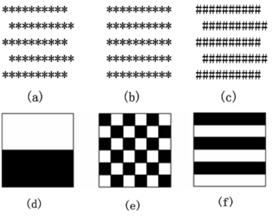
2.4 Texture Analysis

Texture analysis and classification are common tasks in pattern recognition. The main

aim of texture analysis is texture recognition and texture-based shape analysis. The

aim of texture description is to derive some measurements that can be used to classify

a particular texture [Nixon 02]. Texture refers to properties which represent the

surface or structure of an object [Sonka 98], it could be defined as a structure

composed of a large number of more or less ordered similar elements or patterns

without one of these drawing special attention [VanGool 85]. “The notion of texture

appears to depend upon three ingredients: (i) some local ‘order’ is repeated over a

region which is large in comparison to the order’s size, (ii) the order consists in the

nonrandom arrangement of elementary parts, and (iii) the parts are roughly uniform

entities having approximately the same dimensions everywhere within the textured

region.” [Hawkins 69]. Texture comprises texture primitives (also called texels) and is

highly dependent on the number considered (the texture scale). “A Texture primitive

is a contiguous set of pixels with some tonal and/or regional properties, and can be

depicted by its average intensity, maximum or minimum intensity size, shape, etc.”