Online two-section PV array fault diagnosis with optimized voltage sensor locations



Abstract—Photovoltaic (PV) stations have been built widely in the world to utilize solar energy directly. In order to reduce the capital and operational costs, early fault diagnosis is playing an increasingly important role by enabling the long effective operation of PV arrays. This paper analyzes the terminal characteristics of faulty PV strings and arrays, and develops a PV array fault diagnosis technique. The terminal current-voltage curve of a faulty PV array is divided into two sections: a high-voltage and a low-voltage fault diagnosis section. The corresponding working points of healthy string modules, healthy and faulty modules in an unhealthy string are then analyzed for each section. By probing into different working points, a faulty PV module can be located. The fault information is of critical importance for the maximum power point tracking (MPPT) and the array dynamical reconfiguration. Furthermore, the string current sensors can be eliminated while the number of voltage sensors can also be reduced by optimizing voltage sensor locations. Typical fault scenarios including mono-string, multi-string and partial shadow for a 1.6 kW 3×3 PV array are presented and experimentally tested to confirm the effectiveness of the proposed fault diagnosis method.

Index Terms—Fault diagnosis, optimization, photovoltaics, terminal characteristics, voltage sensors.

I. INTRODUCTION

Photovoltaic (PV) systems provide a promising solution to directly utilizing solar energy and are currently gaining in popularity as the technologies are mature and the material costs are driven down [1]-[5]. However, as they are installed in outdoor environments, operational and maintenance costs have always been an issue, demanding some fault diagnosis functions to improve system reliability.

A PV module consists of dozens of PV cells in series connections. A large number of PV modules connected in series form a PV string, which can be further connected in parallel to form a PV array. PV modules are characterized with low power density and low output voltage [6]-[8]. If the PV system is connected to a power grid, a large number of PV modules are needed to connect in series to achieve a high voltage level. Typically, a 400 V bus voltage is required for a 220 V 50 Hz single-phase grid, and a 600 V bus voltage for a three-phase grid. Similarly, a large number of PV strings are also needed to connect in parallel to increase their power level [9][10]. For example, a 20 kW grid-connected PV system generally employs 80 modules to form a 20×4 array (i.e. 20 modules in a string and 4 strings to form an array).

In field conditions, a number of factors can cause the PV array to reduce its output power. In this paper, any cause for this reduction is considered as the “fault”. It can be permanent (such as open-circuits, short-circuits and device aging), or temporary

(such as dust, leave, bird dropping and shadow). A temporary fault can be cleared after a short period of time while a permanent fault would persist over time. Temporary faults can normally be identified by human eyes and thus be cleared through maintenance. Some permanent faults can be seen if the damage is severe while other permanent faults are invisible to the naked eye so that they may propagate and cause the PV modules to deteriorate over time. PV faults can occur in the PV array and generate different effects on the performance and lifetime of the PV system [11]-[16]. Currently, thermal cameras [17]-[23], earth capacitance measurements (ECM) [24] and time domain reflectomery (TDR) [25] are the three popular methods for PV fault diagnosis. Thermal cameras can be employed to detect the temperature characteristics of a PV array under fault conditions. Thermal images can also be linked to the maximum power point tracking (MPPT) algorithm of the PV controller [22]. In practice, a gradual change in the thermal image of the PV module (e.g. due to device aging) poses a technical challenge [23], and high system costs also limit the wide application of thermal cameras. The ECM can locate the disconnection of PV strings while the TDR technology can predict the degradation of the PV array. Nonetheless, both ECM and TDR can only operate offline [24][25]. In practice, online diagnosis methods are highly desired, which can take measurements while the tested device is in operation. To improve this, an automatic supervision and fault detection is proposed in [26][27] based on power loss analysis. However, it requires surrounding environmental information and cannot identify the faulty module. An operating voltage-window is then developed based on the PV string operation voltage and ambient temperature [28]. It can locate the open and short faults but still cannot identify the faulty module from the array. Currently, both offline and online fault diagnosis methods have been developed. Offline diagnosis methods cannot give real-time fault information that is the key factor for PV array optimization operation under fault condition. Current, online fault diagnosis methods suffer from high costs or incapability of locating fault modules. A model-based reconfiguration algorithm is developed in [29] to realize the fault-tolerant operation. But it needs a large number of electrical relays to reconfigure PV arrays. A similar technology, the in-situ rearrangement strategy, can decrease the influence of shadow [30]-[33]. However, its success depends on three conditions: i) a large number of relays are used. ii) the health state of all PV modules should be monitored. iii) high computing resource of the controller is required to calculate complex optimal arrangements. These increase the system cost and control complexity. Paper [34] develops an improved strategy which combines power channels and relays to combat the shadow influence but it also needs the healthy state of PV modules. Paper [35] proposes a fingerprint curve of the PV array under shading

On-Field Two-Section PV Array Fault

conditions to find the key information (e.g. open-circuit and short-circuit points and MPP region) but it cannot locate the faulted modules. Paper [36] presents a fault diagnosis technique using current and voltage sensors but the system cost is quite high. Paper [22] presents a method to use the fault diagnosis information for global MPPT without a need to trace I-V curves. It becomes clear that online fault diagnosis is important because i) it is the prerequisite for any array dynamical reconfiguration. ii) it can provide crucial information for global MPPT; (iii) it contains key state-of-health information useful for system maintenance.

This paper proposes a low cost and online fault diagnosis method with optimized voltage sensor locations that can effectively locate the faulty PV strings and faulty modules. The paper is organized as follows. Section II introduces PV fault mechanisms. Section III illustrates the optimization of sensor locations. Section IV describes the two-section PV array fault diagnosis method. Section V presents experimental results to verify the proposed method, followed by a short conclusion in Section VI.

II. FAULT MECHANISMS

Firstly, it is crucial to understand fault mechanisms prior to developing fault diagnosis techniques.

A. PV string faults

The PV string is the basic structure of a PV array. Fig. 1 presents typical output characteristics of the PV string under faulty conditions; the PV module parameters are listed in Table I. The string includes three modules with non-uniform illumination, the corresponding environment parameters are 850 W/m2_{, 25}o_C; 620 W/m2_{, 25}o_{C; 400 W/m}2_{, 25}o_{C. Each module has uniform} illumination. It can be found that: i) The multi-stage characteristics are caused by the differing output current of each module; ii) In the low voltage diagnosis section, the faulty modules are short-circuited, and the terminal voltage of the corresponding faulty module is zero.

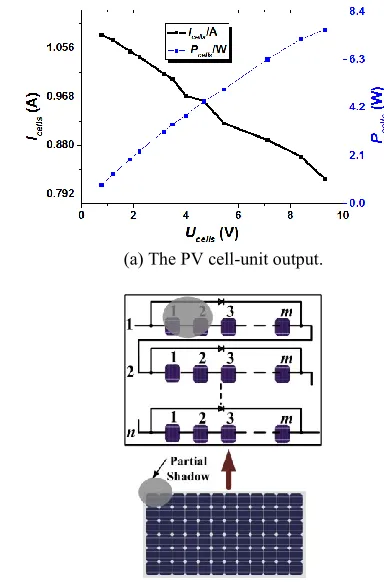
In order to restrict the hot-spots in a PV module, a bypass diode is connected in parallel to PV cells. The corresponding structure is named the cell-unit, which is composed of m PV cells. The PV module is connected in series by n cell units to achieve the high output voltage. Usually, partial shadow is also accrued in one PV module. Due to the cell-unit structure, even though only one cell is faulty (0 W/m2_{), the output power of the cell-unit will} decrease dramatically. Fig. 2(a) presents experimental results of the faulty cell-unit that includes 24 PV cells with one faulty PV cell; the experimental environment parameters are 790 W/m2 _at 24o_{C. The faulty cell is equivalent to a resistance. As the current} increases, the corresponding cell-unit output power is decreased dramatically. For instance, the faulty cell-unit works at 0.96 A, and its output power is 4.75 W (about 10% of the output at healthy condition) and this power reduces to nearly zero when the cell-unit current is higher than 1 A. In order to achieve a global MPP for the PV array, the current is much higher than 1 A under the condition in Fig. 2. Therefore, the output voltage for a faulty cell-unit is effectively negligible, as shown in Fig. 2.

Fig. 1 Output characteristics of the faulty string.

TABLE ISPECIFICATIONS OF THE PV MODULE

Parameter Value Open-circuit voltage 44.8 V Short-circuit current 5.29 A

Power output 180 W

MPP current 5 A

MPP voltage 36 V

Current temperature coefficient 0.037%/K Voltage temperature coefficient 4 Power temperature coefficient 8 Operating cell temperature 46±2°C

Therefore, when a PV module is subjected to partial shading, its terminal output voltage is lower than the healthy module but higher than zero. In Fig. 2(b), the PV module loses one of the cell-units and its output voltage is reduced to 𝑛−1_𝑛 of the output voltage.

(a) The PV cell-unit output.

PV string fault diagnosis can be achieved by measuring the PV module voltage, which changes with the string working point. When the string works in the low voltage diagnosis section, the faulty module can be located because its output voltage is zero (full shadow) or lower than the healthy module (partial shadow).

B. PV array faults

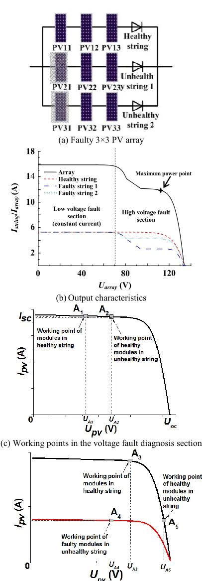
When a PV array is faulted, the faulty module has a lower effective illumination than healthy modules. Take a 3×3 array for example. Fig. 3(a) shows a multi-string faulty condition and Fig. 3(b) shows its I-V characteristics. In Fig. 3(a), the diodes are used to block the reverse current when a fault occurs. The output I-V characteristics can be divided into two sections: a high voltage diagnosis section and a low voltage diagnosis section (constant output current). In the latter section, the faulty module in the faulty string is shorted by bypass diodes where both healthy string and unhealthy string carry the same current. PV string current sensors cannot distinguish the unhealthy string from healthy strings. Nevertheless, the healthy modules in the faulty string have a higher output voltage than the modules in the healthy string, as points A1 and A2 illustrated in Fig. 3(c). The voltage difference between the healthy module in the unhealthy string, and the module in the healthy string can be employed to locate the faulty module.

In this paper, s modules are connected in series to form a PV string and p PV strings are connected in parallel to form a PV array. For a p row s column array, assume that there are x faulted modules in the unhealthy string. In Fig. 3(c), UA1 is the voltage of

a PV module in a healthy string, such as PV11; UA2 is the voltage

of a healthy PV module in an unhealthy string, such as PV22. UA1

and UA2 can be expressed as:

1 array A

U U

s



(1)

2 array A

U U

s x



 ₍₂₎ where Uarray is the output voltage of PV arrays.

The high voltage diagnosis section in Fig. 3(b) is due to a lower solar illumination of the faulty module. The output current of the unhealthy string is limited by the faulty module output current. Therefore, the unhealthy string output current is lower than the healthy string. Since all the modules contribute to electricity generation, there are three working points in two output characteristics. A3 is the working point of modules in the healthy string; A4 is working point of the faulty modules in the unhealthy string; A5 is the working point of normal modules in the unhealthy string; as in Fig. 3(d). Because both A3 and A5 are the working points of a healthy module, they share the same output curve characteristics. Because A4 and A5 are the working points of an unhealthy module and a healthy module in the same string, they have the same output current.

Voltages UA3, UA4 and UA5 for working points A3, A4 and A5 are given by:

3 4 5

(

)

A A A

U

 

s U

 

x U

 

s x

(a) Faulty 3×3 PV array

Maximum power point

Uarray (V)

Istri

ng

/

Iarray

(A

)

18

14

10

6

2

Array Healthy string Faulty string 1 Faulty string 2

Low voltage fault section (constant current)

High voltage fault section

0 40 80 120

(b) Output characteristics

(c) Working points in the voltage fault diagnosis section

(d) Working points in the high-voltage diagnosis section Fig. 3 PV array under fault conditions.

According to the previous analysis, UA4＜UA3＜UA5. This can

array output voltage is between 100~130 V, every module in the healthy string generates electricity and works in the high-voltage diagnosis section. In the unhealthy string, the faulty module cannot generate electricity. Although the healthy modules work in the high-voltage diagnosis section, the unhealthy string still cannot reach the PV array voltage. Therefore the healthy modules in the unhealthy string are effectively open-circuited, similar to the faulted modules. There is neither current flowing in the unhealthy string, nor in the bypass diodes. That is, all the modules in an unhealthy string are open-circuited.

Therefore, the fault diagnosis can be achieved by analyzing the module voltage at different diagnosis sections. This also removes the necessity of current sensors. In this work, the two-stage power conversion [37] is adopted so that the control of the PV system is load independent. That is, the PV’s working point can be chosen at will in the two-stage PV system where the front-end DC-DC converter tracks the desired working point of the PV array; the bus voltage control and the DC-AC inverter control ensure that the grid current is controlled as per the input power.

Fig. 4 Extreme case of the PV array fault.

III. OPTIMIZATION OF SENSOR LOCATIONS

In order to achieve the PV array fault diagnosis, the reading of PV module voltage is needed. Due to the large number of PV modules employed, a large number of voltage sensors are also needed in the first instance.

A. Sensor placement strategy

There are three basic sensor placement methods, as shown in Fig. 5. If every module’s terminal voltage is measured by a voltage sensor by method 1; and the total number of sensors is

ps. In method 2, each voltage sensor measures the voltage between two nodes in the same column of adjacent strings; and (p1)(s1) voltage sensors are needed. In method 3, the electric potential difference of adjacent modules is measured; the corresponding number of sensors is p(s2). The large number of voltage sensors may increase system capital cost and information processing burden. Therefore, the voltage placement method needs to be optimized.

Fig. 6 shows an equivalent PV matrix where a PV module is shown as a dot; the connection line of the adjacent module is represented by a node. The proposed voltage placement strategy is developed by the following steps:

V

V V

V. 5 V

V V

V V

V V V

V V V

V V

V

V

V

V

(a) Method 1 (b) Method 2 (c) Method 3 Fig. 5 Voltage sensor placement methods.

i) All the nodes should be covered by voltage sensors. ii) A sensor can only connect one node in a string.

iii) Voltage sensor nodes cover different isoelectric points from different strings.

iv) If p or s is an even number, each node is connected to and only to one sensor. If both p and s are odd, there is one and only one node to be connected to two different sensors, while each of remaining nodes is connected to one sensor.

Fig. 6 Equivalent matrix.

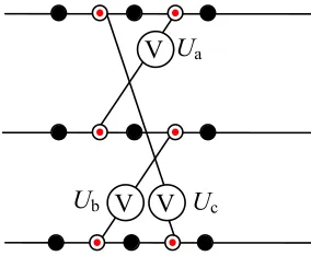
Fig. 7 presents an example of the 3×3 PV array. According to the proposed sensor placement strategy, only three voltage sensors are needed.

U

V

V

V

U

U

Fig. 7 Simplified voltage sensor placement method for a 33 PV array.

TABLE IINUMBER OF VOLTAGE SENSORS USED BY DIFFERENT METHODS

Method 1 2 3 Proposed

No. p s (p-1)(s-1) p(s-2) p(s-1)/2

B. Mathematical model of the proposed sensor placement strategy

The variable 𝑎𝑖𝑗 is defined as the state of the PV module sitting

at the i-th string and j-th module (denoted by (𝑖, 𝑗)) in the 𝑝 × 𝑠 array. If this module is healthy, then 𝑎𝑖𝑗=1, otherwise 𝑎𝑖𝑗=0. The

terminal voltage of the (i, j) module is denoted by 𝑢𝑖𝑗, and the

reading of a voltage sensor connecting the (i, j) module and another module sitting at the (r, k) position is denoted by 𝑅𝑖,𝑗,𝑟,𝑘.

Consider that each string has at least one healthy module. The number of healthy modules in the i-th string equalizes 𝑎𝑖1+

𝑎𝑖2+ ⋯ + 𝑎𝑖𝑠. The terminal voltage 𝑢𝑖𝑗 of the (i, j) module is

equal to a fraction of 𝑈𝑎𝑟𝑟𝑎𝑦, and this fraction is 0 if 𝑎𝑖𝑗 = 0, and

is 1/(𝑎𝑖1+ 𝑎𝑖2+ ⋯ + 𝑎𝑖𝑠) if 𝑎𝑖𝑗 = 1. That is,

𝑢

=

𝑎𝑖1+𝑎𝑖2+⋯+𝑎𝑖𝑠 (4)

Note that the total output voltage of the modules (i, 1), (i, 2),…, and (i, j) is the sum of the terminal voltage of j modules, i.e., 𝑢𝑖1+ 𝑢𝑖2+ ⋯ + 𝑢𝑖𝑗. Similarly the total output voltage of the

modules (r, 1), (r, 2),…, and (r, k) equalizes 𝑢𝑟1+ 𝑢𝑟2+ ⋯ 𝑢𝑟𝑘.

Therefore, the reading of the voltage sensor connecting the (i, j) module and the (r, k) module is calculated as

𝑅𝑖,𝑗,𝑟,𝑘 = (𝑢𝑖1+ 𝑢𝑖2+ ⋯ + 𝑢𝑖𝑗) − (𝑢𝑟1+ 𝑢𝑟2+ ⋯ 𝑢𝑟𝑘)

=

𝑎𝑖1+𝑎𝑖2+⋯+𝑎𝑖𝑠

−

(𝑎𝑟1+𝑎𝑟2+⋯+𝑎𝑟𝑘)𝑈array

𝑎𝑟1+𝑎𝑟2+⋯+𝑎𝑟𝑠 (5)

When the working point of a PV string moves to the high voltage section, the output voltage of the healthy modules increases until reaching the open circuit voltage 𝑈𝑜𝑐. The faulted

modules in the string will equally divide the remaining voltage

𝑈array−(𝑎𝑖1+ 𝑎𝑖2+ ⋯ + 𝑎𝑖𝑠)𝑈𝑜𝑐. The following relations hold for

a string including both healthy and unhealthy modules.

𝑢

= 𝑎

𝑈

+

𝑠−(𝑎𝑖1+𝑎𝑖2+⋯+𝑎𝑖𝑠)

=

𝑠−(𝑎𝑖1+𝑎𝑖2+⋯+𝑎𝑖𝑠)

+

(1−𝑎𝑖𝑗)𝑈array

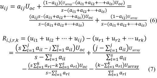
𝑠−(𝑎𝑖1+𝑎𝑖2+⋯+𝑎𝑖𝑠) (6)

𝑅𝑖,𝑗,𝑟,𝑘= (𝑢𝑖1+ 𝑢𝑖2+ ⋯ + 𝑢𝑖𝑗) − (𝑢𝑟1+ 𝑢𝑟2+ ⋯ 𝑢𝑟𝑘)

=(𝑠 ∑ 𝑎𝑖𝑙

𝑗

𝑙=1 − 𝑗∑𝑠𝑙=1𝑎𝑖𝑙)𝑈𝑜𝑐

𝑠 − ∑𝑠𝑙=1𝑎𝑖𝑙 +

(𝑗 − ∑𝑗𝑙=1𝑎𝑖𝑙)𝑈array ∑𝑠𝑙=1𝑎𝑖𝑙

−

𝑠−∑𝑠𝑙=1𝑎𝑟𝑙

−

(𝑘−∑𝑘𝑙=1𝑎𝑟𝑙)𝑈array ∑𝑠𝑙=1𝑎𝑟𝑙 (7)

The reading 𝑅𝑖,𝑗,𝑟,𝑘 at the high voltage section provides extra

equations to solve variable 𝑎𝑖𝑗.

There is a way to design the optimal sensor placement for any 𝑝 × 𝑠 array with ⌈𝑝 × (𝑠 − 1)/2⌉ sensors. If p is an even number, the 𝑝 × 𝑠 array can be divided into 𝑝₂ elements of 2 × 𝑠 arrays. For each 2 × 𝑠 array, it needs to apply the optimal sensor placement method by using 𝑝₂× 𝑠 sensors. If p is odd, the 𝑝 × 𝑠

array consists of one 3 × 𝑠 array and 𝑝−3₂ elements of 2 × 𝑠 arrays. It needs to apply the sensor placement method for these elements and the number of sensors needed is equal to ⌈3 × (𝑠 − 1)/2⌉ +𝑝−3₂ (𝑠 − 1). By considering both even and odd numbers, it can be found that:

⌈3 × (𝑠 − 1)/2⌉ +𝑝−3

2 (𝑠 − 1) = ⌈𝑝 × (𝑠 − 1)/2⌉ (8)

Therefore, the optimal number of sensors can be obtained. IV. TWO-SECTION PV ARRAY FAULT DIAGNOSIS STRATEGY The proposed PV array fault diagnosis strategy is implemented in three steps: locating healthy PV string, locating faulty module in the low-voltage diagnosis section, and in the high-voltage diagnosis section.

A. Locating healthy PV string

The information of healthy strings is useful to identify a faulty module. Thus the first step in fault diagnosis is to locate healthy PV strings. Because of the absence of current sensors in the string, the healthy string cannot be found directly. When a PV array changes from a healthy condition to an unhealthy condition, the voltage sensor can pick up the change.

i) If the voltage sensor reading 𝑅𝑖,𝑗,𝑟,𝑘 always satisfies

𝑅𝑖,𝑗,𝑟,𝑘=𝑗−𝑘_𝑠 𝑈array despite any changes of the working point along

the I-V curve, both i-th and r-th strings are healthy.

ii) If the i-th string is healthy, the sensor reading 𝑅𝑖,𝑗,𝑟,𝑘

satisfies 𝑅𝑖,𝑗,𝑟,𝑘

𝑈array −

𝑗 𝑠= −

𝑎𝑟1+𝑎𝑟2+⋯+𝑎𝑟𝑘

𝑎_𝑟1+𝑎_𝑟2+⋯+𝑎_𝑟𝑠 at low voltage working

points. This can be used to judge the number of faulty modules in the r-th string.

iii) If the i-th string is healthy, and (𝑅𝑖,𝑗,𝑟,𝑘−𝑗_𝑠𝑈array) remains

constant for all working points, there is no current flowing in the

r-th string, i.e., the r-th string is open circuited. This is because that (𝑅𝑖,𝑗,𝑟,𝑘−𝑗_𝑠𝑈array) is equal to the voltage of the first k modules

in the r-th string (i.e. 𝑢𝑟1+ 𝑢𝑟2+ ⋯ 𝑢𝑟𝑘). Whenever there is

current flowing in the r-th string, there will be at least one module works at low voltage working points (e.g., 𝑈array < 𝑈𝑜𝑐). At the

low voltage section, the reading of 𝑢𝑟1+ 𝑢𝑟2+ ⋯ 𝑢𝑟𝑘 is a

function of 𝑈array and cannot remain constant.

B. Locating faulty PV modules in the low-voltage section

TABLE IIISENSOR VOLTAGE OF THE MONO-STRING FULLY FAULTED MODULES

PV31~PV33 Ua Ub Uc

100 Uarray/3 2Uarray/3 Uarray/6

010 Uarray/3 Uarray/6 Uarray/6

001 Uarray/3 Uarray/6 2Uarray/3

110 Uarray/3 2Uarray/3 Uarray/3

011 Uarray/3 Uarray/3 2Uarray/3

101 Uarray/3 2Uarray/3 2Uarray/3

111

000

Uarray/3

Uarray/3

2Uarray/3-Uoc

Uarray/3

2Uoc -Uarray/3

Uarray/3

Note：0: healthy, and 1: faulty.

TABLE IVSENSOR VOLTAGE OF THE MULTI-STRINGS FULLY FAULTED MODULES

PV11~PV13/PV21~PV23 Ua Ub Uc

100/100 Uarray/2 Uarray/6 2Uarray/3 010/100 Uarray/2 Uarray/6 Uarray/6 001/100 Uarray Uarray/6 Uarray/6 100/010 Uarray/6 Uarray/6 2Uarray/3 010/010 Uarray/6 Uarray/6 Uarray/6 001/010 Uarray/2 Uarray/6 Uarray/6 100/001 0 2Uarray/3 2Uarray/3

010/001 0 2Uarray/3 Uarray/6 001/001 Uarray/2 2Uarray/3 Uarray/6 110/100 0 Uarray/6 2Uarray/3 101/100 Uarray Uarray/6 2Uarray/3 011/100 Uarray Uarray/6 Uarray/3

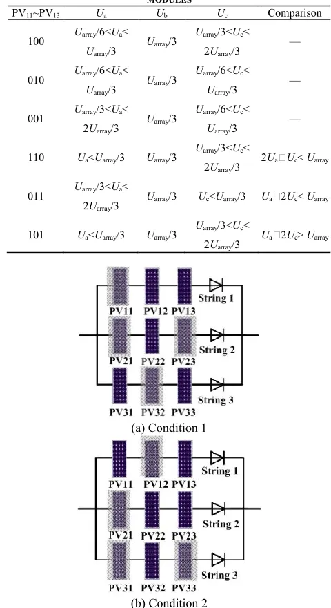
In practice, partial shading is a very common fault [2]-[3][5][12]-[14][22]-[33]. This is illustrated in detail in Table V. Both Tables III and V are concerned with PV module faults. Tables III deals with the fully-faulted module where all cell-units are faulted while Table V shows a partially faulted module including some faulted cell-units. Their output voltages are zero and non-zero, respectively.

C. Locating faulty PV module in the high-voltage diagnosis section

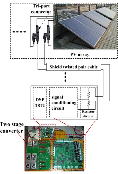
If all the PV strings are faulty, the eigenvalues of Tables III-V may be the same as other faulty conditions. This can lead to misjudgment in locating faulty modules.

For example, two types of the unhealthy 3×3 PV array with the same sensor placement strategy are presented in Fig. 8. PV11, PV21, PV23 and PV32 are faulty at fault condition 1; PV12, PV21, PV31 and PV33 are faulty at condition 2. Two fault conditions give the same voltage reading in the low-voltage diagnosis section, which is Uarray/2. In order to discriminate the

two conditions, the high voltage diagnosis section is employed to find the actual faulty modules.

As analyzed previously, when the PV array works in the high diagnosis voltage section, the faulty modules in string 2 are open-circuited while strings 1 and 3 can still operate. In a low-voltage section all the healthy modules in the array generate electricity and the faulty modules are shorted. The voltage value is different between the low-voltage and the high voltage sections, as

illustrated in Table VI. By changing the diagnosis section from low to high, different eigenvalues can be obtained to locate faulty modules.

TABLE V SENSOR VOLTAGE OF THE MONO-STRING PARTIALLY FAULTED MODULES

PV11~PV13 Ua Ub Uc Comparison

100 Uarray/6<Ua<

Uarray/3 Uarray/3

Uarray/3<Uc<

2Uarray/3 —

010 Uarray/6<Ua<

Uarray/3 Uarray/3

Uarray/6<Uc<

Uarray/3 —

001 Uarray/3<Ua<

2Uarray/3 Uarray/3

Uarray/6<Uc<

Uarray/3 —

110 Ua<Uarray/3 Uarray/3 Uarray/3<Uc<

2Uarray/3 2Ua Uc< Uarray

011 Uarray/3<Ua<

2Uarray/3 Uarray/3 Uc<Uarray/3 Ua 2Uc< Uarray

101 Ua<Uarray/3 Uarray/3 Uarray/3<Uc<

2Uarray/3 Ua 2Uc> Uarray

(a) Condition 1

(b) Condition 2 Fig. 8 The 3×3 array under two fault conditions.

TABLE VI EIGENVALUE UNDER DIFFERENT FAULT DIAGNOSIS SECTIONS

Fault condition Diagnosis section Ua Ub Uc 1 Low voltage _{Uarray/2 Uarray/2 Uarray/2}

2 Low voltage _{Uarray/2 Uarray/2 Uarray/2}

1 High voltage _{Uarray/2-Uoc 2Uoc-Uarray/2 Uarray/2}

2 High voltage _{Uarray/2 Uarray/2-Uoc 2Uoc-Uarray/2}

D. Implementation of the two-section fault diagnosis strategy

module can be located directly by the eigenvalue table in the low-voltage diagnosis section. If there does not exist a healthy string, both the low-voltage fault diagnosis and high-voltage fault diagnosis are needed to locate faulty modules.

Monitor values from voltage sensor

Are all values normal? Y

N Is there a healthy

string?

Low voltage area fault diagnosis

Low voltage area fault diagnosis Y

Locate faulty module

High voltage area fault diagnosis

Locate faulty module

Fig. 9 Flowchart of the two-section fault diagnosis.

V. EXPERIMENTAL TESTS

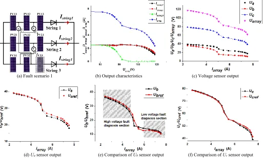
A 3×3 PV array and a signal conditioning system are built to verify the proposed fault diagnosis technique, as shown in Fig. 10. In this figure, resistor dividers are employed as differential voltage sensors to eliminate the grounding issue, tri-port connectors and shield twisted pair cables are used to transmit the voltage signal. In the signal conditioning circuit, the electrical isolation of sensor signals is achieved by using a linear optical coupling (HCNR201) to avoid the interaction of earth and ground connections. The voltage readings are processed by the conditioning circuit and then input to DSP TMS320F2812. The PV modules are the same for simulation, and the environment illumination is recorded by TS1333R. In the experiment, typical fault scenarios are studied and the sensor readings are compared with eigenvalues in the high-voltage and low-voltage diagnosis sections to check the effectiveness of the proposed fault diagnosis technique.

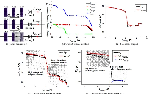
Fig. 11 shows the mono-string mono-module fault diagnosis. In the fault scenario 1 (see Fig. 11(a)), the voltage sensor connection method is identical to that in Fig. 7. The illumination is 550 W/m2 _{and the temperature is 15℃. The P33 PV module is} cast by shadow manually to emulate a partial-shading fault. Uaref,

Ubref and Ucref are the reference voltages for sensors a, b and c,

respectively, under the fault condition. Fig. 11(b) shows the I-V

characteristics of faulty PV arrays. Due to the fault on module P33, string 3 cannot generate electricity in the output voltage range 82~120 V. Fig. 11(c) presents the sensor output voltage. In the low-voltage diagnosis section (10~70V); the sensor a output voltage is Uarray/3 (as shown in Fig. 11(d)). This is a normal

output voltage and the corresponding strings are healthy. That is, strings 1 and 2 connected by this sensor are healthy, which coincides with fault scenario 1 in Fig. 11(a). Fig. 11(e) illustrates the high-voltage and voltage diagnosis sections. In the low-voltage section, the reference eigenvalue is Uarray/6; and in the

high-voltage section, it is 2Uarray/3-Uoc. The fact that the sensor b

output is close to the reference value also verifies the proposed diagnosis method. The reference eigenvalue of Uc is 2Uarray/3; and the corresponding sensor c output also agrees with the reference eigenvalues. There is a slight deviation between Ua, Ub and Uc

and their reference values. This is caused by the diode voltage drop and the minor product irregularity between PV modules. From the sensor output results and information in Table III, the fault type is classified as “001”. The faulty module is P33 that also agrees with fault scenario 1 (Fig. 11(a)).

signal conditioning circuit DSP

2812 Tri-port connector

PV array

Resistor divider

Shield twisted pair cable

Two stage converter

(a) Fault scenario 1 (b) Output characteristics (c) Voltage sensor output

(d) Ua sensor output (e)Comparison of Ub sensor output (f)Comparison of Uc sensor output

Fig. 11 Mono-string mono-module fully faulted diagnosis.

(a) Fault scenario 2 (b) Output characteristics

(c) Comparison ofsensor outputs Ua and Ub. (d) Sensor output voltage

(a) Fault scenario 3 (b) Output characteristics (c) Ua sensor output

(d) Comparisonof sensor output Uc (e)Comparisonof sensor output Ub

Fig. 13 Mono-string multi-module fault diagnosis.

Fig. 12 shows the diagnosis of the multi-string mono-module fault. In fault scenario 2, the illumination is 580 W/m2 _{and the} temperature is 25℃. Module P11 in string 1 and P33 in string 3 are cast by partial shadow manually. Fig. 12(b) presents the I-V characteristics of the faulty PV array. When faults occur in modules P11 and P33, strings 1 and 3 cannot generate electricity in the range of 82~120 V. In the low-voltage section, the sensors

a and b have the same output (Ua=Ub=Uarray/6), as illustrated in

Fig.12(c). The voltage sensors a and b also satisfy the rule for locating healthy strings. Therefore, string 2 is diagnosed as being healthy which coincides with the fault scenario in Fig. 12(a). Fig. 12(d) shows the sensor c output curves. It can be seen that there is a healthy string, and the values of Ua, Ub and Uc are Uarray/6,

Uarray/6 and Uarray, respectively, in the low-voltage diagnosis

section. The faulty modules identified are P11 and P33.

In fault scenario 3 (Fig. 13(a)), the illumination is 610 W/m2 _at 30℃. P32 and P33 in string 3 are cast by partial shadow and full shadow, respectively. Fig. 13(b) shows the output characteristics. String 3 can only generate electricity at 0~60 V. As presented in Fig. 13(c), Ua =Uarray/3 in the whole output voltage range,

indicating strings 1 and 2 are both healthy. In the low-voltage section of Fig. 13(d), Uc matches the reference value 2Uarray/3,

verifying that P33 is faulty. In the high-voltage section, Uc= 2Uoc

-Uarray/3. Therefore, either P31 or P32 is faulty. Fig. 14(e) presents

the output characteristics for sensor b. The corresponding output is equal to -Uarray/3 in the low-voltage range, proving that P32

module is faulty and P31 module is healthy.

From the analysis of three fault scenarios for a 3×3 PV array, the proposed fault diagnosis strategy is proven be effective.

For small-scale or low-voltage arrays, passive voltage sensors (e.g. resistor dividers) can be employed. Given that 16 channels are available for analog-digital (A/D) conversion in DSP TMS320F28335, there might not need for additional A/D chips. For large-scale PV systems at high voltages, Hall-effect voltage sensors (e.g. LEM LV25-P) are required. These sensors can be powered by the PV cell-unit directly. Nonetheless, they also need long sensor cables to transmit the voltage results unless wireless sensor networks are used [38][39]. Clearly, the cost of the fault diagnosis equipment and computational complexity handling for more extended PV arrays and large PV arrays will be increased. Given the gain in reduced voltage sensors and increased solar power production, the total capital cost is justified by using the proposed technique.

It needs to point out that this is a proof-of-concept work and its technology readiness level (TRL) is between 3-4. Ideally, the developed technology will eventually lead to a new product, in place of existing converters for PV systems. However, it can also be integrated into the exiting commercial converters.

i) If commercial converters allow for updating their software programs, the developed algorithm can be implemented into the control program of the front-end DC-DC converter and voltage sensors need to add to the system for voltage measurement. For fault diagnosis, the reference voltages of PV arrays in the low-voltage and high-low-voltage fault diagnosis areas are firstly chosen (0.3 and 0.9 times of the open-circuit PV array voltage in this work, respectively). The difference (error) between the PV array output voltage and the reference voltage is the input to the PI controller and its output is the duty cycle of the DC-DC converter.

their software programs, an extra DC-DC converter is needed and its output is connected across the DC-link capacitor. This arrangement bypasses the first stage of the commercial converter and fault diagnosis can be conducted when the PV system is operational.

VI. CONCLUSION

PVs are a cost-sensitive market. Online fault diagnosis is key to the success of the PV array reconfiguration and the global MPPT. This paper has proposed a low-cost online PV array fault diagnosis with optimized voltage sensor locations. This work can help increase productivity and reduce the capital and maintenance costs by reducing the number of sensors and by developing an effective fault diagnosis technique.

When compared to existing methods in the literature, this work has made the following improvements:

i) String current sensors are removed and the number of voltage sensors is also reduced by optimizing the location of voltage sensors.

ii) An online two-section fault diagnosis method is developed to locate faulty PV modules.

iii) The state of health information from this work can be also used for the MPPT and PV array dynamical reconfiguration.

REFERENCES

[1] Y. A. Mahmoud, W. Xiao, H. H. Zeineldin, “A parameterization approach for enhancing PV model accuracy,” IEEE Trans. Ind. Electron., vol. 60, no.12, pp. 5708-5716, 2013.

[2] B. N. Alajmi, K. H. Ahmed, S. J. Finney, B. W. Williams, “A maximum power point tracking technique for partially shaded photovoltaic systems in microgrids,” IEEE Trans. Industrial Electronics, vol. 60, no. 4, pp. 1596-1606, April 2013.

[3] L. Gao, R. A. Dougal, S. Liu, and A. P. Iotova, “Parallel-connected solar PV System to address partial and rapidly fluctuating shadow conditions,” IEEE

Trans. Ind. Electron., vol. 56, no. 5, pp. 1548-1556, May 2009.

[4] N Femia, G Petrone, G Spagnuolo, M Vitelli,” A technique for improving P&O MPPT performances of double-stage grid-connected photovoltaic systems,” IEEE Trans. Ind. Electron., vol. 56, no. 11, pp. 4473-4482, Nov. 2009.

[5] K. Ishaque, and Z. Salam, “A deterministic particle swarm optimization maximum power point tracker for photovoltaic system under partial shading condition,” IEEE Trans. Ind. Electron., vol. 60, no. 8, pp. 3195-3206, Aug. 2013.

[6] M. Boztepe, F. Guinjoan, G. Velasco-Quesada, S. Silvestre, A. Chouder, E. Karatepe, “Global MPPT scheme for photovoltaic string inverters based on restricted voltage window search algorithm,” IEEE Trans. Ind. Electron., vol. 61, no. 7, pp. 3302-3312, Jul. 2014.

[7] K. Ding, X. Bian, H. Liu, T. Peng, “A MATLAB-Simulink-based PV module model and its application under conditions of nonuniform irradiance,” IEEE

Trans. Energy Convers., vol. 27, no. 4, pp. 864-872, Dec. 2012.

[8] G Petrone, G Spagnuolo, M Vitelli, “Analytical model of mismatched photovoltaic fields by means of Lambert W-function,” Solar energy

materials and solar cells, vol. 91 no. 18, pp. 1652-1657, Nov. 2007.

[9] Y. Hu, Y. Deng, Q. Liu, X. He, “Asymmetry three-level grid-connected current hysteresis control with varying bus voltage and virtual over-sample method,” IEEE Trans. Power Electronics, vol. 29, no. 6, pp. 3214-3222, Jun. 2014.

[10] Y. Liu, B. Ge, H. Abu-Rub, and F. Z. Peng, “An effective control method for three-phase quasi-Z-source cascaded multilevel inverter based grid-tie photovoltaic power system,” IEEE Trans. Ind. Electron., vol. 61, no. 12, pp. 6794-6802, Dec. 2014.

[11] S. Djordjevic, D. Parlevliet, P. Jennings, “Detectable faults on recently installed solar modules in Western Australia” Renewable Energy, vol. 67, pp. 215-221, 2014.

[12] A. Maki, S. Valkealahti, “Effect of photovoltaic generator components on the number of MPPs under partial shading conditions,” IEEE Trans. Energy

Conversion, vol. 28, Issue 4, pp.1008-1017, 2013.

[13] M. Z. S El-Dein, M. Kazerani, M. M. A. Salama, “Optimal photovoltaic array reconfiguration to reduce partial shading losses,” IEEE Trans.

Sustainable Energy, vol. 4, Issue 1, pp. 145-153, 2013.

[14] E. V. Paraskevadaki, S. A. Papathanassiou, “Evaluation of MPP voltage and power of mc-Si PV modules in partial shading conditions,” IEEE Trans.

Energy Conversion, vol. 26, Issue 3, pp. 923-932, 2011.

[15] H. A. Lauffenburger, R. T. Anderson, “Reliability terminology and formulae for photovoltaic power systems,” IEEE Trans. Reliability, vol. R-31, Issue 3, pp. 289-295, 1982.

[16] L. H. Stember, W. R. Huss, M. S. Bridgman, “A methodology for photovoltaic system reliability & economic analysis,” IEEE Trans.

Reliability, vol. R-31, Issue 3, pp. 296-303, 1982.

[17] C. Buerhopa, D. Schlegela, M. Niessb, C. Vodermayerb, R. Weißmanna, C. J. Brabeca, “Reliability of IR-imaging of PV-plants under operating conditions,” Solar Energy Materials and Solar Cells, vol. 107, pp. 154-164, 2012.

[18] Y. Hu, B. Gao, G.Y. Tian, X. Song, K. Li, X. He. “Photovoltaic fault detection using a parameter based model,” Solar Energy, vol. 96, pp. 96-102, Oct. 2013.

[19] A. Krenzinger, A. C. Andrade, “Accurate outdoor glass thermographic thermometry applied to solar energy devices,” Solar Energy, vol. 81, pp. 1025-1034, 2007.

[20] M. Simon and E. L. Meyer, “Detection and analysis of hot-spot formation in solar cells,” Solar Energy Materials and Solar Cells, vol. 94, no. 2, pp. 106-113, 2010.

[21] J. Kurnik, M. Jankovec, K. Brecl and M. Topic, “Outdoor testing of PV module temperature and performance under different mounting and operational conditions,” Solar Energy Materials & Solar Cells, vol. 95, pp. 373-376, 2011.

[22] Y. Hu, W. Cao, J. Wu, B. Ji, D. Holliday, “Thermography-based virtual MPPT scheme for improving PV energy efficiency at partial shading conditions,” IEEE Trans. Power Electron. vol. 29, no. 11, pp. 5667-5672, Jun. 2014.

[23] Z. Zou, Y. Hu, B. Gao, W. L.Woo and X. Zhao, “Study of the gradual change phenomenon in the infrared image when monitoring photovoltaic array,”

Journal of Applied Physics, vol. 115, no. 4, pp. 1-11, 2014.

[24] T. Takashima, J. Yamaguchi, K. Otani, T. Oozeki, K. Kato, “Experimental studies of fault location in PV module strings,” Solar Energy Materials and

Solar Cells, vol. 93 issues. 6-7, pp. 1079-1082, Jun. 2009.

[25] R. A. Kumar, M. S. Suresh, J. Nagaraju, “Measurement of AC parameters of gallium arsenide (GaAs/Ge) solar cell by impedance spectroscopy,” IEEE

Trans. Electron Devices, vol. 48, issue 9, pp. 2177-2179, 2001.

[26] A. Chouder, S. Silvestre, “Automatic supervision and fault detection of PV systems based on power losses analysis,” Energy Conversion and

Management, vol. 51, issue 10, pp. 1929-1937, Oct. 2010.

[27] S. Silvestre, A. Chouder, E. Karatepe, “Automatic fault detection in grid connected PV systems,” Solar Energy, vol. 94, pp. 119-127, Aug. 2013. [28] N. Gokmen, E. Karatepe, S. Silvestre, B. Celik, P. Ortega, “An efficient fault

diagnosis method for PV systems based on operating voltage-window,”

Energy Conversion and Management, vol. 73, pp. 350-360, Sep. 2013.

[29] X. Lin, Y. Wang, D. Zhu, N. Chang and M. Pedram, “Online fault detection and tolerance for photovoltaic energy harvesting systems,” the 2012 IEEE/ACM International Conference on Computer-Aided Design

(ICCAD), San Jose, USA, pp. 1-6. 2012.

[30] D. Nguyen, B. Lehman. “An adaptive solar photovoltaic array using model-based reconfiguration algorithm,” IEEE Trans. Ind. Electron., vol. 55, no. 7, pp. 2644-2654, Jul. 2008.

[31] J. P. Storey, P. R. Wilson, and D. Bagnall, “Improved optimization strategy for irradiance equalization in dynamic photovoltaic arrays,” IEEE Trans.

Power Electron., vol. 28, no. 6, pp. 2946-2956, Jun. 2013.

[32] G. Velasco-Quesada, F. Guinjoan-Gispert, R. Pique-Lopez, M. Roman-Lumbreras, and A. Conesa-Roca, “Electrical PV array reconfiguration strategy for energy extraction improvement in grid-connected PV systems,”

IEEE Trans. Ind. Electron., vol. 56, no. 11, pp. 4319-4331, Nov. 2009.

[33] Y. Wang, X. Lin, Y. Kim, N. Chang, and M. Pedram, “Architecture and control algorithms for combating partial shading in photovoltaic systems,”

IEEE Trans. Computer-Aided Design Integr. Circuits Syst., vol. 33, no. 6, pp.

917-929, Jun. 2014.

[34] S. Jonathan, R. W. Peter, and B. Darren, “The optimized-string dynamic photovoltaic array,” IEEE Trans. Power Electron., vol. 29, no. 4, pp. 1768-1776, Apr. 2014.

[36] Y. Hu, H. Chen, R. Xu, R. Li. “Photovoltaic (PV) array fault diagnosis strategy based on optimal sensor placement,” Proceedings of the CSEE, vol. 31, issue 33, pp. 19-30, 2011.

[37] B. Yang, W. Li, Y. Zhao and X. He, “Design and analysis of a grid-connected photovoltaic power system,” IEEE Trans. Power Electron., vol. 25, no. 4, pp. 992-1000, Apr. 2010.

[38] P. Guerriero, V. d’Alessandro, L. Petrazzuoli, G. Vallone, and S. Daliento, “Effective real-time performance monitoring and diagnostics of individual panels in PV plants,” the 4th International Conference on Clear Electrical

Power (ICCEP), Alghero, Italy, pp. 14-19. 2013.

[39] P. Guerriero, G. Vallone, M. Primato, F. Di Napoli, L. Di Nardo, V. d’Alessandro, S. Daliento, “A wireless sensor network for the monitoring of large PV plants,” the International Symposium on Power Electronics,

Electrical Drives, Automation and Motion (SPEEDAM), Ischia, Italy, pp.