PT-symmetry breaking in complex nonlinear wave equations and their deformations

City, University of London Institutional Repository

Citation: Cavaglia, A., Fring, A. & Bagchi, B. (2011). PT-symmetry breaking in complex

This is the accepted version of the paper.

This version of the publication may differ from the final published

version.

Permanent repository link: http://openaccess.city.ac.uk/13893/

Link to published version: http://dx.doi.org/10.1088/1751-8113/44/32/325201

Copyright and reuse: City Research Online aims to make research

outputs of City, University of London available to a wider audience.

Copyright and Moral Rights remain with the author(s) and/or copyright

holders. URLs from City Research Online may be freely distributed and

linked to.

City Research Online: http://openaccess.city.ac.uk/ [email protected]

arXiv:1103.1832v1 [math-ph] 9 Mar 2011

PT

-symmetry breaking in complex nonlinear wave

equations and their deformations

Andrea Cavaglia•_{, Andreas Fring}• _{and Bijan Bagchi}◦

• _{Centre for Mathematical Science, City University London,}

Northampton Square, London EC1V 0HB, UK

◦ _{Department of Applied Mathematics, University of Calcutta,}

92 Acharya Prafulla Chandra Road, Kolkata 700 009, India

E-mail: [email protected], [email protected], [email protected]

Abstract:_{We investigate complex versions of the Korteweg-deVries equations and an Ito}

type nonlinear system with two coupled nonlinear fields. We systematically construct ra-tional, trigonometric/hyperbolic, elliptic and soliton solutions for these models and focus in particular on physically feasible systems, that is those with real energies. The reality of the energy is usually attributed to different realisations of an antilinear symmetry, as for instance PT-symmetry. It is shown that the symmetry can be spontaneously broken in two alternative ways either by specific choices of the domain or by manipulating the parameters in the solutions of the model, thus leading to complex energies. Surprisingly the reality of the energies can be regained in some cases by a further breaking of the symmetry on the level of the Hamiltonian. In many examples some of the fixed points in the complex solution for the field undergo a Hopf bifurcation in the PT-symmetry breaking process. By employing several different variants of the symmetries we propose many classes of new invariant extensions of these models and study their properties. The reduction of some of these models yields complex quantum mechanical models previously studied.

1. Introduction

to regard certain complex quantum mechanical Hamiltonians also as perfectly acceptable self-consistent descriptions of physical systems [4], in the sense that they possess real energy eigenvalue spectra and well defined unitary time-evolution (see [5, 6, 7] for recent reviews). To consider pseudo/quasi Hermitian systems provides a very clear conceptual view in this respect as it makes use of a similarity transformation towards a Hermitian Hamiltonian system for which everything is well defined in a standard conventional sense, although such transformations do not exist for all types of such systems. A more radical view is to give a direct meaning to the non-Hermitian Hamiltonians without any reference to the Hermitian system. This latter point of view has to be taken in order to explain recent experiments in which non-Hermitian systems are studied on optical lattices, see e.g. [8], as the observed gain and loss can not be explained in a purely Hermitian setting. A further experimental realization has recently been proposed for graphene nanoribbons, where non-Hermitian Hamiltonians arise as effective Hamiltonians [9].

Largely inspired by the study of the quantum systems, also classical complex systems have been investigated recently. Naturally one may view them too in various ways, either as directly meaningful or only sensible when transformed to a real system. Many classical models have already been investigated from these various perspectives, such as complex extensions of standard one particle real quantum mechanical potentials [10, 11, 12, 13], non-Hamiltonian dynamical systems [14], chaotic systems [15] and deformations of many-particle systems such as Calogero-Moser-Sutherland models [16, 17, 18, 19]. These inves-tigations led to new insights into the quantum theories based on the features found in these classical models, such as tunneling behaviour [13, 20], band structures [21] and even a complex generalizations of Bohr’s correspondence principle has been formulated [22].

Extensions of field theories of nonlinear wave type, such as Korteweg-deVries (KdV) equations [23, 24, 25] and closely related models [26, 27, 28, 29] have also been investigated. These type of models will be the main subject of our investigations in this manuscript.

Pseudo or quasi-Hermiticity are often equivalent to a simultaneous parity and time reversal, so-called _PT-symmetry. Remarkably this property, or more general antilinear symmetry [30], of quantum mechanical systems is already visible on the classical level. It is known for more than fifty years that when this symmetry is unbroken the reality of the spectrum of the theory is guaranteed. Unbroken refers here to the property that

[_PT, H] = 0 and _PTΦ = Φ, (1.1)

Here we will trace these properties on the classical level and use the reality of the classical energy as a criterium to select physically meaningful complex models including their boundary and initial conditions. The role of Φ in (1.1) is in this case played by the solution of the classical field equation of motion, say u(x, t). For a given Hamiltonian density_H depending onu(x, t) the energy on the interval x_∈[₋a, a] is computed by

E =

Z a

−aH

[u(x)]dx=

I

ΓH

[u(x)]du

ux

. (1.2)

Here and throughout the manuscript we use the standard convention ux ≡du/dx. When

the system possesses periodic solutions, that is whenu(a) =u(₋a) along a path Γ in the complexu-plane, we can employ the alternative contour integral version in (1.2). A simple argument [24] shows that the energy in the interval x _∈ [₋a, a] is guaranteed to be real if the symmetry property _H∗_{[u(x)] = H[u(−x)] holds for the Hamiltonian density. We}

will present here some unexpected examples of real energy solutions for which neither of the relations in (1.1) hold, i.e. the _PT-symmetry is broken for the Hamiltonian and the solutions.

Here we will investigate two different types of complexified wave equations. First of all we study in section 2 the most immediate way to complexify wave equations by introduc-ing complex boundary values and initial conditions for the KdV-system. We investigate systematically the traveling wave and soliton solutions. We study complex trajectories in the complex plane of the KdV-field especially with regard to their properties under

PT-symmetry breaking. In section 3 we employ the different types of _PT-symmetry as a construction principle to propose new extended versions of the KdV-system. We inves-tigate the new models in a similar fashion as their undeformed counterparts. Particular attention is paid to the question of what kind of conditions will lead to physical models, in the sense that they possess real energies. In section 4 we study the effect of complex boundary conditions and initial values on a nonlinear system with two fundamental fields coupled to each other, which is referred to as Ito system for some specific parameter choice. We also investigate the _PT-symmetry properties of these models. Due to the presence of an additional field when compared with the KdV-system we can identify four different versions of_PT-symmetry being realised in these systems, which we exploit in section 5 to construct new models. We study them from similar points of view as the previous ones. We draw our conclusions in section 6.

2. Complex Korteweg-deVries equation

Complex extensions of the KdV equation have been investigated already some time ago for instance in [32, 33, 34, 35]. However, _PT-symmetry has only been utilized recently in [23, 24, 25] in order to understand some of their properties and in particular to construct new models. The standard KdV system is known to be a Hamiltonian system with density

HKdV =−

β

6u

3₊ γ

2u 2

leading to the Korteweg-deVries equation in the form

ut+βuux+γuxxx= 0. (2.2)

Usually the constantsβandγ are chosen to be real, but here we allow them to take complex values, thus including the possibility for u(x, t) to be complex. _PT-symmetry may then be realised in two alternative ways as

PT+ :x7→ −x, t7→ −t, i7→ −i, u7→u forβ, γ∈R, (2.3)

PT− :x7→ −x, t7→ −t, i7→ −i, u7→ −u foriβ, γ∈R, (2.4)

both possibilities guaranteeing that _PT± :_HKdV 7→ HKdV holds. The underlying models respect one of the two symmetries and are therefore different as they correspond to two distinct choices of the coupling constant which may, however, be related by a simple rotation inu. Nonetheless, with regard to possible deformations to be discussed below this second symmetry allows to construct different types of new models.

A crucial feature of the model to be acceptable as physically consistent is the reality of the energy (1.2). In case of the Hamiltonian density_HKdV the reality of the energy (1.2) is guaranteed for the two possibilities u∗_{(x) = u(−x) when β, γ ∈} R _{or u}∗_{(x) = −u(−x)}

when iβ, γ _∈R_{, resulting fromPT+ or PT−, respectively.}

2.1 _PT-symmetric, spontaneously broken and broken solutions

Let us now see which complex boundary conditions and initial values are physically per-missible. In order to establish this, we first briefly recall how the traveling wave solutions of the KdV-equations of motion may be constructed systematically. Integrating (2.2) twice leads to the equation

u2_ζ = 2

γ

κ2+κ1u+

c

2u

2₋β

6u 3

=:λP(u) (2.5)

with integration constants κ1, κ2 ∈ C and P(u) denoting a third order polynomial in u multiplied by an overall constantλ. A further integration yields

±√λ(ζ₋ζ₀) =

Z

dup1

P(u), (2.6)

where we made the usual assumption that the fieldu(x, t) acquires the form of a traveling wave u(x, t) =u(ζ) withζ =x₋ctandcdenoting the wave speed. In complete generality this is an elliptic integral, but it is instructive to generate simpler solutions by systemati-cally making some specific assumptions on the factorization of the polynomialP(u). This solution method may then be extended to the deformed cases.

Demanding specific boundary conditions will impose further restrictions or might be entirely incompatible with certain factorizations of P(u). For instance, in case we wish to implement vanishing asymptotic boundary conditions for u and its derivatives, the once integrated version of equation (2.2) and (2.5) implies

lim

In the following we will study the solutions in the complexu-plane. For this purpose it is useful to separate u into its real and imaginary part uR and uI, respectively, and decouple (2.5) into two first order differential equations in these variables

uR_ζ =_±Re

√

λ

q

P(uR_+iuI₎

and uI_ζ =_±Im

√

λ

q

P(uR_+iuI₎

. (2.8)

In this set up we may then apply many of the techniques which have been developed for two dimensional dynamical systems, see for instance [36]. Most immediate is the application of the linearisation theorem at some fixed point uf, converting the nonlinear system into

uR ζ

uI_ζ

!

= J(uR, uI)

u=uf

uR ζ

uI_ζ

!

, (2.9)

with Jacobian matrix

J(uR, uI)

u=uf =



±

∂Re[√λ√P(u)]

∂uR ±

∂Re[√λ√P(u)]

∂uI

±∂Im[ √

λ√P(u)]

∂uR ±

∂Im[√λ√P(u)]

∂uI  

u=uf

. (2.10)

We denote the eigenvalues ofJ(u=uf) byj1,j2. Provided the system (2.9) is simple and Reji6= 0 the linearisation theorem applies, stating that the phase portraits of the systems

(2.8) and (2.9) are qualitatively the same in some neighbourhood of the fixed point uf.

The ten similarity classes for 2_×2-matrices fully characterizing all possible behaviours for the fixed points of (2.8) are reported for reference in appendix A.

2.1.1 Rational solutions

FactorizingP(u) at first in the simplest way asP(u) = (u₋A)3 with one constantAleaves no freedom when solving (2.5), as all constants are fixed

λ=₋β

3γ, κ1=− c2

2β, κ2 = c3

6β2 and A= c

β. (2.11)

Clearly asymptotically vanishing boundary conditions (2.7) are only possible for a static solution withc= 0. The evaluation of the expression (2.6) produces for this factorization the rational solution

u(ζ) = c

β −

12γ

β(ζ₋ζ₀)2, (2.12)

with additional integration constantζ_{0 ∈}C_{. Takingζ}

0 as purely imaginary maintains the

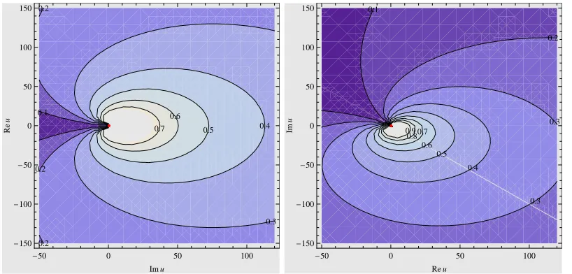
PT-symmetry of the solution, whereas any real part may be compensated by a shift inζ, which is kept to be real. Independently of the parameter choice, asymptotically all rational solutions of the type (2.12) end up at limζ→±∞u(ζ) =c/β, as we can also observe in figure

1.

Focussing at first on the _PT-symmetric scenario, we notice that while keeping the speed of the wave c real there are two possible choices for the conjugation leading to physical solutions, namely u∗_{(ζ) = u(−ζ) when iζ}

0, β, γ ∈ R or u∗(ζ) = −u(−ζ) when

different initial conditionsζ₀. We have taken the plus and minus sign in (2.6) for the upper and lower half plane, respectively. We observe that for a specific branch the pointAin the

u-plane appears to be either a stable or an unstable improper asymptotic fixed point. We adopt here the notion for the characterizations of fixed points from the linearisation (see appendix A for a classification), despite the fact thatuζ is not a meromorphic function and

the system is not easily linearized. This implies that only the choice with different branches for the upper and lower half will give rise to closed orbits as depicted. For increasing ζ, they run either out of the fixed point in the upper half plane and into it in the lower half or vice versa. The crossing of the trajectories with the real line is easily computed to be at u(0) =c/β+ 12γ/β(Imζ₀)2. This makes it evident that only complex trajectories may be closed, whereas the real solution is the only trajectory drifting off to minus infinity.

Since the rational solution (2.12) does not have any free parameter left, as specified in (2.11), there is no possibility to break the_PT-symmetry spontaneously for this type of solution. We may, however, break the _PT-symmetry completely directly on the level of the Hamiltonian by fully complexifying β or γ, an example of which is depicted in figure 1b. As expected we observe that the symmetry u∗_{(ζ) =u(−ζ) has been lost, but instead}

the trajectories are almost symmetric about the line passing the two points A and u(0), which are now both located away from the real axis. However, the nature of the fixed point, being either an unstable or stable improper node, has not changed.

0.1

0.2

0.2 0.2

0.3 0.4 0.5

0.6 0.7

-50 0 50 100

-150 -100 -50 0 50 100 150

Im u

Re

u

0.1

0.2

0.3

0.3 0.4

0.5 0.6 0.7 0.8 0.9

-50 0 50 100

-150 -100 -50 0 50 100 150

Re u

Im

u

Figure 1: Complex rational solutions of the KdV equation for different values of purely complex initial conditionsζ0: (a)PT-symmetric solutions forc= 1,β = 2,γ= 3 andA= 1/2; (b) Broken PT-symmetric solutions forc= 1,β = 2 +i2,γ= 3 and A= (1−i)/4. Different trajectories are characterized by different initial conditions ζ0. Some values for the imaginary part of Imζ0 <1

are indicated on the trajectories. The unresolved white region corresponds to values for Imζ0>1.

Throughout this manuscript we label panels from the left to the right as (a), (b), (c), etc.

Considering the expression for the energy (1.2) it is evident that it will be real when we have the symmetry u∗_{(x) = u(−x). We also compute the expression explicitly for the}

computed to

Ea=−ac

2

3β2

c+ 36γ

a2_−ζ2 0

+ 72γ 2

15β2

"

10c a3+ 3aζ2₀

a2_−ζ2 0

3 −

48γ a5+ 10a3ζ2₀+ 5aζ4₀

a2_−ζ2 0

5

#

.

(2.13) EvidentlyEais real even when iζ0, β, γ ∈Ror iζ0, iβ, γ∈Rand complex otherwise, that is for the _PT-symmetric and broken _PT-symmetric case, respectively.

2.1.2 Trigonometric/hyperbolic solutions

As the next possibility for the factorization we specify P(u) = (u₋A)2(u₋B) involving now two constantsA and B, thus leaving one of them at our disposal when solving (2.5)

λ=₋ β

3γ, κ1 = A

2(βA−2c), κ2=

A2

6 (3c−2βA) and B = 3c

β −2A. (2.14)

Having now some freedom in the choice of the constants one may ask which ones are the most natural to use for the symmetry breaking. As we will see the constants A and B

have a direct physical meaning and it appears therefore natural to view them as the free parameters to tune for a concrete model with fixed coupling constantsβ, γ, rather than the integration constantsκ1 or κ2 emerging more indirectly without immediate interpretation. By (2.7) vanishing asymptotic boundary conditions require the choiceA= 0.

In general, the solution to (2.6) produces in this case the trigonometric/hyperbolic solution

u(ζ) =B+ (A₋B) tanh2

1 2

√

A₋B√λ(ζ₋ζ₀)

. (2.15)

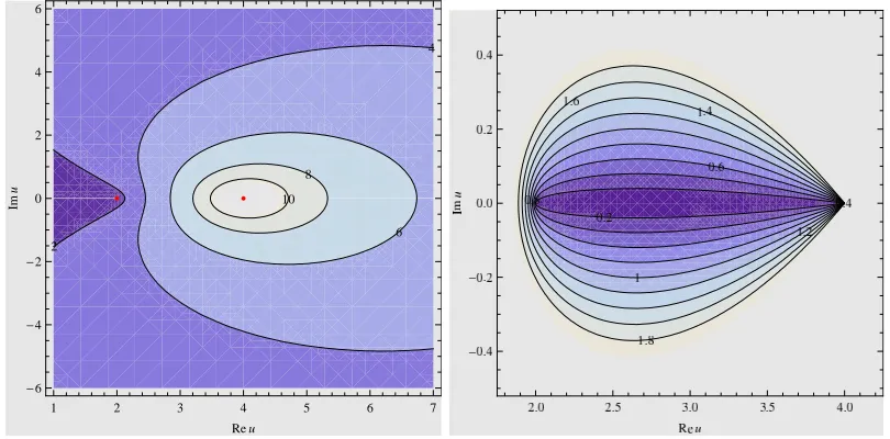
Let us first discuss the_PT-symmetric scenario for which all constants are taken to be real except for ζ₀, which we still allow to be complex. When in that case either A < B,λ >0 or A > B, λ < 0 we obtain a periodic solution with period T = 2π/(p_|A₋B_|p_|λ_|) as depicted in figure 2a. The closed trajectories surround the point A, whereas the point

B is situated on its outside, following from the fact that on the real axis we always have

u(ζ) < B or u(ζ) > B, in the respective cases. This behaviour is also confirmed by the linearisation (2.9) at the fixed point A. ParameterizingA₋B=rABeiθAB and λ=rλeiθλ

the Jacobian (2.10) is easily computed to

J(u)_|u=A= ±

√_r

ABrλcos

₁

2(θAB+θλ)

∓√rABr_λsin

₁

2(θAB+θλ)

±√rABrλsin₂1(θAB+θλ) ±√rABrλcos₂1(θAB +θλ)

!

, (2.16)

with eigenvalues

j1 =±√rABrλexp

i

2(θAB+θλ)

and j2 =±√rABrλexp

−₂i(θAB+θλ)

. (2.17)

Clearly for the two cases here, that is A < B,λ > 0 or A > B,λ < 0, the eigenvalues of the Jacobian are purely complex, i.e. j1/2 =±i

p

|A₋B_|p_|λ_|, indicating that the point

For this periodic case we may also compute the energy ET for one period T from

−π/p_|A₋B_|p_|λ_|to π/p_|A₋B_|p_|λ_|analytically to

ET =

I

ΓH

[u(ζ)]du

uζ

=

I

Γ

H[u]

√

λ√u₋B(u₋A)du=−π

r

βγ

3

A3

√

A₋B. (2.18)

Here the contour Γ is taken to be any complex trajectory resulting for iζ_{0 ∈} R_{. Then}

(2.18) follows from Cauchy’s residue theorem and the fact that B will always be outside the contour Γ. We find that the energy is real and takes the same value for all trajectories independently of the concrete choice for the initial conditionζ₀. Notice that the energy for the real solution, i.e. ζ_{0 ∈}R_{, can not be computed in such an easy way as in that case Γ}

does not form a closed contour. Thus demanding_PT-symmetry leads inevitably to purely complex initial value conditions and constitutes a natural ”ǫ-prescription” to deform the real solution with the purpose to compute the energy for one period.

For the remaining possibilities A > B, λ > 0 or A < B, λ < 0 all solutions tend asymptotically to A, which we depict for some examples in figure 2b. The linearisation (2.9) at the fixed pointAyields in these cases the two degenerate real eigenvaluesj1=j2 =

p

|A₋B_|p

|λ_| or j1 =j2 = −

p

|A₋B_|p

|λ_| for J depending on the plus or minus sign in (2.8), respectively. The Jacobian (2.16) is diagonalisable in these cases and therefore A

is an unstable or stable star node. As for the rational solutions, this implies that only the choice with different branches for the upper and lower half will give rise to closed orbits as seen in figure 2b. Now the energies can not be computed in a simple manner as for the periodic case since the singularity at A is situated on the contour.

2

4

6 8

10

1 2 3 4 5 6 7

-6 -4 -2 0 2 4 6

Re u

Im

u

Figure 2: Complex trigonometric/hyperbolic solutions of the KdV equation: (a) PT-symmetric periodic solutions withc= 1,β = 3/10,γ = 3,A= 4,B = 2 andT = 2√15π; (b) PT-symmetric asymptotically constant solutions withc= 1,β = 3/10,γ=−3, A= 4 andB= 2.

parameters at our disposal. From (2.14) and (2.15) it is clear that when 2βκ1+c2 <0 the constant A becomes complex and we no longer have the propertyu∗_{(ζ) =u(−ζ) ensuring}

the reality of the spectrum. The nature of the fixed point is now changed again to an unstable or stable focus depending on whether Reji >0 or Reji <0, respectively. Thus

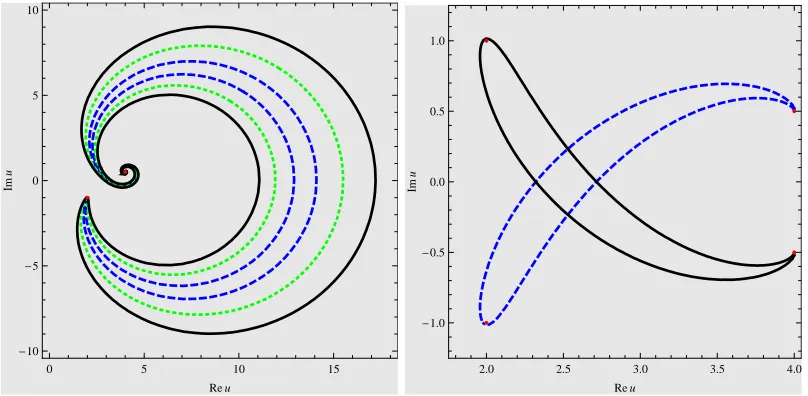
once again closed orbits are obtained with the choice of different branches for the upper and lower half plane. This means of course that the periodic solution ceases to be periodic. The energiesET for one period in the periodic solution corresponding to the two choices

A, B, ζ₀ and A∗_{, B}∗_{, ζ}∗

0 occur in complex conjugate pairs. This is the typical scenario for spontaneously broken _PT-symmetry, i.e. the Hamiltonian is still _PT-symmetric but the solutions to the Schr¨odinger equation in the quantum case and in the classical case to the equation of motion, are not. Formula (2.18) may still be used in this case for the computation of the energy even though the singularities are moved away from the real axis as they still lie within the contour. Once again the result does not depend on the choice of

ζ₀. We depict some trajectories for this type of spontaneous symmetry breaking in figure 3. The conjugate solution is simply obtained by a reflection about the real axis, as shown explicitly for the asymptotically constant solution in panel (b).

0 5 10 15

-10 -5 0 5 10

Re u

Im

u

2.0 2.5 3.0 3.5 4.0

-1.0 -0.5 0.0 0.5 1.0

Re u

Im

u

Figure 3: Complex trigonometric/hyperbolic solutions of the KdV equation: (a) Spontaneously broken PT-symmetry of the periodic solution with c = 1, β = 3/10, γ = 3, A = 4 +i/2 and B = 2−ifor Imζ0 = 0.5 solid (black), Imζ0= 0.3 dotted (green) Imζ0= 0.1 dashed (blue); (b)

Spontaneously brokenPT-symmetry of the asymptotically constant solution withc= 1,β= 3/10, γ=−3 forA= 4−i/2,B= 2 +iImζ0=−0.5 solid (black)andA= 4 +i/2,B= 2−i, Imζ0= 0.5

dashed (blue).

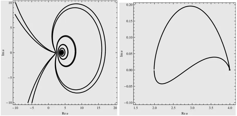
Finally, there is of course also the possibility to break_PT-symmetry directly for the Hamiltonian itself. For instance when β /_∈R _{and/or γ /∈}R _{we expect the energies to be}

complex. In that case the complex conjugate energy would be obtained by considering a new type of Hamiltonian with β∗, γ∗ _{and thus it does not arise from within one specific}

model. We depict an example trajectory for this scenario in figure 4.

qualitatively the same as the one for the spontaneously broken case, namely a stable or unstable focus. This behaviour follows from the eigenvalues (2.17), which indicate that there is no distinction at this point in whether the complexification of theji result from a

spontaneous or a complete breaking of the _PT-symmetry. Note that the trajectories still close even though this is not shown in figure 4a, but this may be seen on a larger scaled plot. We find a similar behaviour for the fixed point of the broken asymptotic solution as depicted in figure 4b.

-10 -5 0 5 10 15 20

-10 -5 0 5 10

Re u

Im

u

1.5 2.0 2.5 3.0 3.5 4.0

-0.10 -0.05 0.00 0.05 0.10 0.15 0.20

Re u

Im

u

Figure 4: Complex trigonometric/hyperbolic solutions of the KdV equation: (a) Broken PT -symmetry of the periodic solution withA= 4,B = 2,c= 1,β= 3/10,γ= 3 +i/2 and Imζ0= 6;

(b) Broken PT-symmetry of the asymptotically constant solution with A = 4, B = 2, c = 1, β= 3/10,γ= 3 +i/2 and Imζ0= 1/2.

So far we have simply broken the symmetry by choosing some more or less random complex value for γ. However, we can also carry out this process in a more controlled fashion producing periodic motion and even some non-Hermitian non-_PT-symmetry cases with real energies. First of all we observe from eigenvalues of the Jacobian (2.10) that the fixed point A becomes a centre when θAB +θλ = π, which is also compatible with the

solution (2.15) from which we notice that a periodic motion occurs when λ(A₋B) <0. This allows for complex values of the parametersβ, γ, A andB. Combining this constraint with the last equation in (2.14) leads to

A= sinθγ

|β_|sin (θγ−θβ −θA)

exp (iθA). (2.19)

Thus, for a given model, that is forany fixed values ofβ andγwe obtain a periodic motion around the point A, given by the expression in (2.19) for any value ofθA. Indeed this is

the case as we observe for instance in figure 5a. When using the constraintθAB+θλ =π

for the periodic motion in the expression for the energy (2.18) we find

ET =−

π

3

βA3

p

Hence, demanding that the energy is to be real leads to the further constraint 3θA+θβ =

0, π. Implementing this in (2.19) yields

ET ∈R forA=

sinθγ

|β_|sin (θγ−2θβ/3)

exp

−iθβ

3

. (2.21)

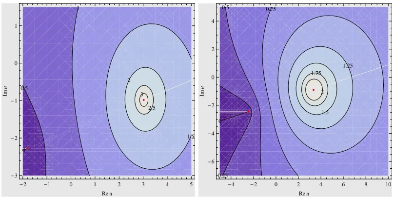
This means for a given model, that is for any fixed values of β and γ we can find a point A, given by the expression in (2.21), around which the trajectory is periodic and the corresponding energy is real. This holds irrespective of whether β and γ are real or complex, or in other words whether the_PT-symmetry is intact or completely broken. In figure 5b we depict an example solution of (2.21) corresponding to a periodic motion with completely broken_PT-symmetry but real energy. An obvious question to ask at this point is whether by breaking this symmetry the system has acquired a new kind of anti-linear symmetry, which could serve to explain the reality of the energy. A systematic study of this more general issue will be presented elsewhere.

0 0.5

1

1.5 2

2.5 3

-2 -1 0 1 2 3 4 5

-3 -2 -1 0 1

Re u

Im

u

0

0.25

0.5 0.75

1 1.25

1.5 1.75

2

-4 -2 0 2 4 6 8 10

-6 -4 -2 0 2 4

Re u

Im

u

Figure 5: Complex trigonometric/hyperbolic solutions of the KdV equation with completely bro-kenPT-symmetry: (a) Periodic solution with complex energyET =−10.518 +i1.666 forc = 1,

β = 1/2 exp(iπ/4), γ = 1/3 exp(iπ/3), A = √3 sin(11π/60) exp(−iπ/10) ≈ 3.025−i0.983 and B = 6 exp(−iπ/4)−2√3 sin(11π/60) exp(−iπ/10) ≈ −1.806−i2.277; (b) Periodic solution with real energy ET =−4π for c = 1, β = 1/2 exp(iπ/4), γ = 1/3 expiπ/3, A = 2

√

3 exp(−iπ/12)≈ 3.346−i0.896 and B=−√6(1 +i)≈ −2.449−i2.449.

In general we observe from the various cases studied in this subsection that when we let the parameters vary one of the fixed points for the periodic solution undergoes a Hopf bifurcation, i.e. it changes its behaviour from a stable focus to a centre and then to an unstable focus. As we can see from (2.17) this behaviour is governed by the sign of_±cos₁

2(θAB+θλ)

2.1.3 Elliptic solutions

Next we specifyP(u) = (u₋A)(u₋B)(u₋C) with three constants A,B and C leaving two constants at our disposal when solving (2.5)

λ= ₋β

3γ, κ1=

1 6

β(A2+AC+C2)₋3c(A₋C)

, (2.22)

κ2 =

AC

6 [3c−β(A+C)] and B = 3c

β −(A+C). (2.23)

Vanishing asymptotic boundary conditions reduce this case to the previous one as by (2.7) they require either A=B = 0,A =C = 0 or B =C = 0. The evaluation of (2.6) yields in this case the elliptic solution

u(ζ) =A+ (B₋A) ns2

1 2

√

B₋A√λ(ζ₋ζ₀)

A₋C A₋B

, (2.24)

with ns(z_|m) being one of the Jacobi elliptic functions. Thereforeu(ζ) is a double periodic function

u(ζ) =u(ζ+ω1+ω2) (2.25)

with periods

ω1=

8

√

B₋A√λK

A₋C A₋B

and ω2 =i

16

√

B₋A√λK

C₋B A₋B

. (2.26)

Here K(m) denotes a complete elliptic integral of the first kind. As expected we recover the previous case when two of the constantsA, B, C coincide as in these cases the periods become dependent on each other, i.e. limA→Bω1/ω2 = 1/2 sign(C−A), limA→Cω1/ω2 =

−i_∞ and limB→Cω1/ω2= 0.

Studying at first the _PT-symmetric solutions, we find periodic solutions encircling some of the fixed points. For instance in figure 6 we depict an example in which the fixed points A and B are encircled, whereas C is situated outside of the trajectories. Different types of scenarios are also expected, changing for instance the sign in γ will lead to a periodic orbit surrounding the pointsB and C.

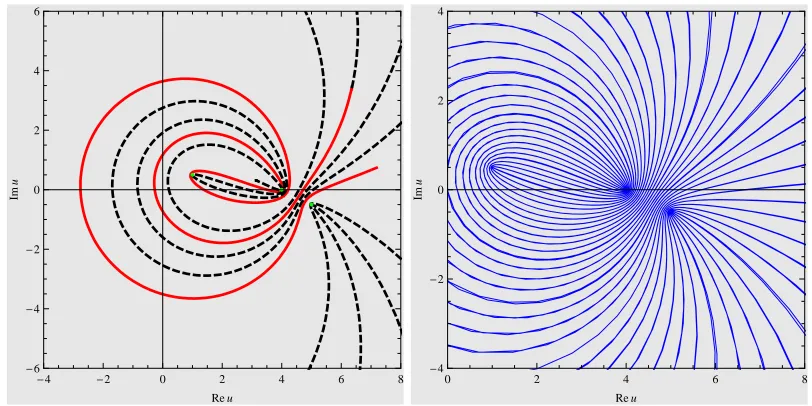
Next we break the_PT-symmetry spontaneously by complexfying the free parameters of the solutions. We find that the periodic trajectories open up and cease to be periodic. In figure 7a we trace part of the trajectory to illustrate the behaviour. Starting at the point u(₋64)_≈7.19 +i0.74 the trajectory passes down between the pointsA and B and moves then up again surrounding once the pointsCandAin a clockwise sense. Thereafter it encircles C once more but instead of moving around A it passes inbetween C and A

surroundingAin an anti-clockwise sense. It keeps progressing in an anti-clockwise manner encircling C before passing from below between the points A and B reaching the point

3 3

4

5

6 7

8 9

-4 -2 0 2 4

-4 -2 0 2 4

Re u

Im

u

0 0.5

1 1.5

2

2.5 3_3.5

-40 -20 0 20 40

-40 -20 0 20 40

Re u

Im

u

Figure 6: PT-symmetric complex elliptic solutions of the KdV equation with A = 1, B = 3, C= 6,c= 1,β = 3/10,γ=−3 for different values of Imζ0.

-4 -2 0 2 4 6 8

-6 -4 -2 0 2 4 6

Re u

Im

u

0 2 4 6 8

-4 -2 0 2 4

Re u

Im

u

Figure 7: Spontaneously broken PT-symmetric complex elliptic solutions of the KdV equation for Imζ0= 6 withA= 4,B= 5−i/2,C= 1 +i/2,c= 1,β = 3/10 andγ= 3: (a) −64≤ζ≤18

solid (red) and 18< ζ≤200 dashed (black); (b)−200< ζ <1400.

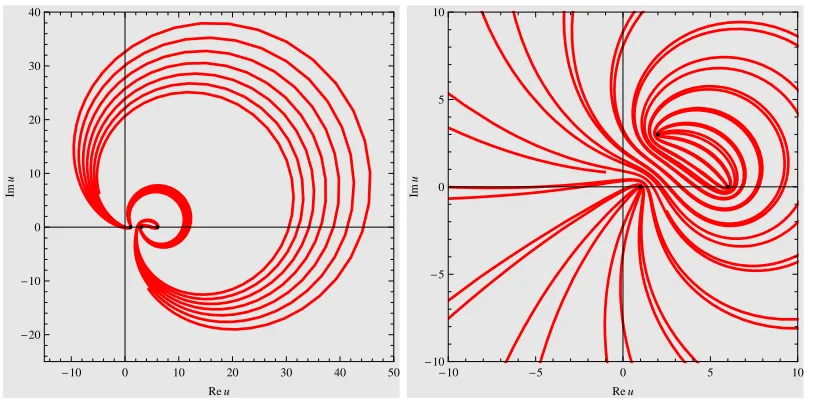
Finally we may also break the_PT-symmetry completely by complexfying the param-eters of the modelβ or/andγ. Examples for such a scenario are depicted in figure 8. The behaviour is similar to the one of the spontaneously broken case, i.e. the periodic motion has turned into open trajectories with a noncompact limit set. Increasing the range for ζ

will fill the depicted part of the phase space similarly as in the spontaneously broken _PT -symmetry case, thus suggesting a chaotic behaviour, albeit once again we do not observe the typical sensitivity towards the initial conditions.

-10 0 10 20 30 40 50 -20

-10 0 10 20 30 40

Re u

Im

u

-10 -5 0 5 10

-10 -5 0 5 10

Re u

Im

u

Figure 8: BrokenPT-symmetric complex elliptic solutions of the KdV equation for Imζ0= 6: (a)

A= 1,B = 3,C= 6,c= 1,β = 3/10 andγ= 3 + 2ifor−200≤ζ≤200;(b)A= 1,B = 2 + 3i, C= 6,c= 1,β = 3/10−i/10 andγ= 3 for−200≤ζ≤200.

reference [12]. This is not surprising as formally the differential equations solved in there for the quantum mechanical setting for the potential V _∼x3 _{are special cases of our more} general treatment when making the identification u_→x and ζ _→tfor our traveling wave equation. With the further identifications

κ1= 0, κ2 =γE, β = 6cg and γ =−c (2.27)

equation (2.5) converts precisely into the quantum mechanical Hamiltonian

H =E = 1 2p

2₊1

2x

2_−gx3_{, (2.28)}

treated in [12]. The identification (2.27) explains why no analogue to our rational solution was found in [12], since κ1 = 0 implies c = 0 and therefore the vanishing of κ2, i.e. the confining potential, andA. However, as can be seen from (2.14) there should be an analogue to our trigonometric solution with energy E = ₋4c3_/γβ2 _{when setting A = 2c/β. This} energy depends on the coupling constant and is of course not freely choosable as in the elliptic case presented in this section whereκ2 is a free parameter. More potentials of the type treated in [12] can be obtained systematically from the deformations discussed below. The new elliptic solutions recently found for generalized shallow wave equations [37] are expected to exhibit a similar behaviour as the solution discussed in this subsection.

2.1.4 Soliton solutions

There exist various techniques to construct soliton solutions. Here we briefly recall and apply Hirota’s direct method [38] for that purpose. The starting point of this approach is Hirota’s bilinear form, which reads in general

withp(D) being a polynomial in the Hirota derivatives, i.e.Dxf ·g=fx·g−f·gx where

the dot ”_·” indicates the noncommutative nature of the productf_·g. The soliton solutions to (2.29) may then be constructed perturbatively order by order inε from the expansion

τ =

∞

X

n=0

εnτn. (2.30)

Defining the functionτ(x, t) via the relation

u(x, t) = 12γ

β (lnτ)xx, (2.31)

the KdV-equation (2.2) can be brought into Hirota’s bilinear form

6γ β γD

4

x+DxDt

τ_·τ = 0. (2.32)

We have set here the integration constant to zero. Taking the zeroth order solution to be

τ0 = 1 the first order tau-function results toτ1(x, t) = exp(p1x−γp31t+φ1) and we obtain the well-known one-soliton solution up to this order

u(x, t) = 3γp 2 1

βcosh2₁

2(p1x−γp31t+φ1)

. (2.33)

A _PT-symmetric variant of this solution is depicted in figure 9a. As expected the origin in theu-plane is an asymptotic fixed point, reached for x_{→ ±∞} or t_{→ ±∞}.

Breaking the_PT-symmetry in various ways yields more unexpected results. Regarding

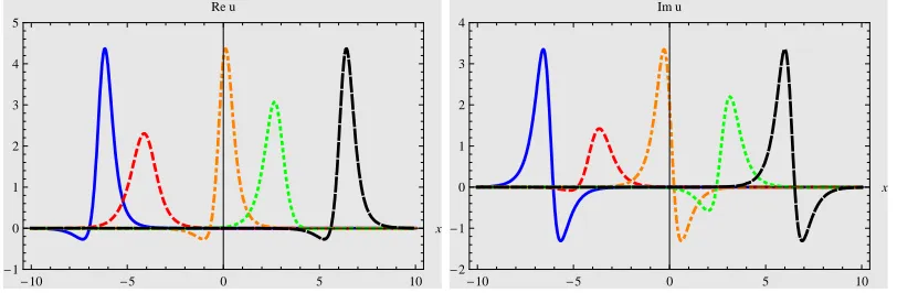
p1, φ1,ζ0 as parameters of the solution and β, γ as model defining constants, their com-plexification constitutes a spontaneous or complete _PT-symmetry breaking, respectively. The corresponding solutions in the u-plane appear as distorted versions of the symmetric case, as can be seen in figure 9b. An interesting feature of the broken complex solution is that, unlike its real counterpart, the soliton does not maintain its overall shape while traveling. Instead, it becomes a breather and regains its shape after a certain distance ∆x

and certain amount of time ∆tgoverned by the equation

u(x+ ∆x, t) =u(x, t+ ∆t). (2.34)

Separating γ,p1 into their real and imaginary part as γ =γr+iγi and p1 =pr+ipi, we

can solve (2.34) for the one-soliton solution (2.33) to

∆t =

2πpr

p4

i −p4r

γ_i−2pipr p2i +p2r

γ_r, (2.35)

∆x = 2π

pi 3p2r−p2i

γ_i+ 2πpr 3p2i −p2r

γ_r p4

i −p4r

γ_i−2pipr p2i +p2r

γ_r . (2.36)

The speed of the soliton is therefore given by

v =₋∆x ∆t

= 3p2_{i −}p2_r

γ_r−pi p

2

i −3p2r

γ_i pr

0.0 0.2 0.4 0.6 0.8 1.0 -0.4

-0.2 0.0 0.2 0.4

Re u

Im

u

0 2 4 6

-2 0 2 4 6

Re u

Im

u

Figure 9: Complex one-soliton solution of the KdV-equation at fixed time t = −2: (a) PT -symmetric solution withβ= 6,γ= 1,p1= 1.2 forφ=i0.3 solid (blue),φ=i0.8 dashed (red) and

φ=i1.1 dotted (black); (b) BrokenPT-symmetric solution withβ = 6,γ= 1 +i0.4,p1= 1.2 for

φ=i0.3 solid (blue),φ=i0.8 dashed (red) andφ=i1.1 dotted (black).

Clearly for the_PT-symmetric solution the shape will be the same in theu-plane even at different times, whereas the complex solution will change its shape as we observe in figure 9. In figure 10 we observe that the one-soliton changes its shape while progressing in time but regains it after ∆t=−π/2 for the chosen values.

-10 -5 0 5 10

-1 0 1 2 3 4 5

x

Re u

-10 -5 0 5 10

-2 -1 0 1 2 3 4

x

Im u

Figure 10: Complex spontaneously broken one-soliton solution of the KdV-equation withβ = 6, γ = 1 +i/2,p1 = 2, φ =i0.8 and ∆t =−π/2 for different times t =−π/2 solid (blue), t =−1

dashed (red),t= 0 dasheddot (orange),t= 0.7 dotted (green), andt=π/2 dasheddotdot (black) (a) real part; (b) imaginary part.

Proceeding to the next order inεwe compute the two soliton solution to

u(x, t) = 24γ

P6

k=0ck(−1)kpk2p61−k

β(p1+p2)4

h

2 cosh 1₂(η₁₋η₂)

+e−η1 2 −

η2 2

eη1+η2_(p1−p2)4

(p1+p2)4 + 1

i2 (2.38)

where we abbreviated η_i=pix−γpi3t+φi fori= 1,2 with

0.0 0.5 1.0 1.5 2.0 -0.20

-0.15 -0.10 -0.05 0.00 0.05 0.10 0.15 0.20

Re u

Im

u

0.0 0.5 1.0 1.5 2.0

-0.15 -0.10 -0.05 0.00 0.05 0.10 0.15

Re u

Im

u

Figure 11: PT-symmetric two-soliton solutions of the KdV equation forβ = 6, γ= 1,p1= 1.2,

p2 = 2.2,φ1 =i0.1 and φ2 =i0.2. (a)t =−2 solid (blue), t=−0.2 dashed (red),t = 0.2 dotted

(black); (b)t= 0.3 dotted (black),t= 0.8 dashed (red),t= 2.0 solid (blue).

We observe in figure 11 the typical scenario for soliton scattering, albeit in the complex plane. For large negative time the two-solitons are separated, indicated here by two indi-vidual one-soliton solutions resembling the type depicted in figure 9 touching each other only in the asymptotic point at the origin. In the scattering regime the two solutions merge in a non_PT-symmetric manner until they separate again for large positive time, acquiring once again their individual one-soliton shape.

0 2 4 6

-2 0 2 4 6

Re u

Im

u

0 2 4 6

-2 0 2 4 6

Re u

Im

u

Figure 12: Broken PT-symmetric two-soliton solutions of the KdV equation for β = 6, γ = 1 +iπ/8,p1= 2(2/3)1/3,p2= 2,φ1=i0.1 andφ2=i0.2. (a)t=−4 solid (blue),t=−3.5 dashed

(red),t=−2.dotted (black); (b)t= 0.7 solid (blue), t= 2 dashed (red),t= 8 dotted (black).

For the values in figure 12 the periods for the one-soliton breather to regain its shape withp1 and p2 are computed by (2.35) to be ∆t1=−3 and ∆2t =−2, respectively. Indeed

we observe in figure 12a that one of the solitons has recovered its shape comparing the solutions att=₋4 and t=₋2. In figure 12b we observed that both solitons have almost regained their original shape passing from t= 2 to t = 8, that is after 2∆1

t = 3∆2t. The

slight discrepancy visible in the figure is due to the well known time delay occurring in a multi-soliton scattering, see e.g. [39].

with formula (1.2)

E1s=−

36γ3p5₁

5β2 , (2.40)

exhibiting the typical behaviour, that is being real for the_PT-symmetric case and complex for the (spontaneously) broken scenario. The integral (1.2) withu(x, t) given by two-soliton solution (2.38) is not easily computed analytically. For large values of time we compute numerically real energies for _PT-symmetric solutions, for instance for the values used in figure 11 we obtain E2s ≈ −10.8049 =E1s(p1) +E1s(p2). On the other hand we compute complex energies for broken_PT-symmetric solutions, such as for the values used in figure 12 for which we evaluateE2s≈ −7.8876−i9.4327 =E1s(p1) +E1s(p2). This means that in all scenarios the energy of the two-soliton equals the sum of the two separate one-solitons.

3. _PT-symmetric deformations of the KdV equation

Employing the standard arguments used in the study of non-Hermitian Hamiltonian sys-tems with real eigenvalues, we may now _PT-symmetrically deform the Hamiltonian and maintain the possibility to have well defined physical systems, e.g. we still obtain real energies resulting from the new models despite their non-Hermitian nature. The general principle is simply to deform _PT-anti-symmetric quantities, that means if we have the property_PT :φ(x, t) _{7→ −}φ(x, t) for some fieldφ(x, t), we define a deformation map δε :

φ(x, t) _{7→ −}i[iφ(x, t)]ε_{. The undeformed case is recovered in the limit ε = 1. The new}

quantity will remain anti-_PT-symmetric with the crucial difference that the overall minus sign is generated from the antilinear nature of the _PT-operator, i.e. i_{7→ −}i, rather than from φ(x, t) _{7→ −}φ(x, t). This means for the Hamiltonian resulting from the density (2.1) we can make use of either of the two possibilities

δ+_ε :ux 7→ux,ε:=−i(iux)ε or δ−ε :u7→uε:=−i(iu)ε, (3.1)

depending on whether we choose u(x, t) to be _PT-symmetric or _PT-anti-symmetric, re-spectively. Accordingly we define the deformed models with some suitable normalisation by the following Hamiltonian densities

H+ε =−

β

6u

3₋ γ

1 +ε(iux)

ε+1_{, and H}−

ε =

β

(1 +ε)(2 +ε)(iu)

ε+2₊γ 2u

2

x, (3.2)

with corresponding equations of motion

ut+βuux+γuxxx,ε= 0 and ut+iβuεux+γuxxx= 0, (3.3)

respectively. The Hamiltonian _H+_ε was proposed in [24] whereas _H−

ε corresponds to a

complex version of the generalized KdV equation. For the higher deformed derivatives we use here the notationuxx,ε:= ∂xux,ε,uxxx,ε:=∂x2ux,ε,. . . , unx,ε :=∂xn−1ux,ε, which means

we only deform the first derivative and keep acting on it with∂x to define the higher order

derivatives. On the level of the equation of motion we could also deform the dispersion term proportional toβ, as investigated in [23] for the KdV-equation. However, such deformations do not lead to Hamiltonian systems and the question of how_PT-symmetry may be utilized in this scenario remains an open issue.

3.1 The _H+

ε-models

Proceeding similarly as in the previous section, we integrate the first equation in (3.3) twice and obtain the deformed version of equation (2.5)

u(_ζn)= exp

iπ

2(ε+ 1)(1−ε+ 4n)

[λεP(u)]

1

1+ε, (3.4)

where we abbreviated λε = −β(1 +ε)/(6γε) and denote different branches by n. The

polynomial P(u) is identical to the one introduced in (2.5), which means we can employ the same factorization as in the previous section. Integrating once more yields

ζ(n)₋ζ₀ = exp

iπ

2(ε+ 1)(ε−1 + 4n)

Z

du 1

[λεP(u)]

1 1+ε

. (3.5)

We may now proceed as before and specify further the form ofP(u). As for the caseε= 1, in some specific cases we succeed to compute the remaining integral and subsequently solve the resulting equation for u, thus obtaining u(ζ). However, even when this is not possible analytically we can still investigate (3.5) numerically forall cases by viewingζas a function of the complex variableu and plotting the contours of Im[ζ(u)] =ζ₀ in the u-plane, while taking special care about the different Riemann sheets labeled byn. One should distinguish here these type of Riemann sheets from those arising due to the technique employed in our solution procedure. Consideringζ as a function of u, as we do in some intermediate steps, will introduce new branch cuts which are sometimes seen in our figures, e.g. figure 27b. However, we do not attribute any meaning to them in the u-plane. Genuine branch cuts can always be distinguished from the “technical” ones by the fact that they have to be connected to the fixed points which are branch points.

3.1.1 Rational solutions

We start with the same assumption as in the previous section, namely P(u) = (u₋A)3, which will impose the same constraints (2.11) for the factorization. The case ε = 2 is special since we may take the root 1/3 in this case. Integrating (3.5) and solving the result foru we find

u(n)(ζ) =A+ exp

"

−ie −2

3inπ 22/3

β γ

1/3

(ζ₋ζ₀)

#

. (3.6)

For the remaining integer values ε_∈Z_{\{2}we can compute also a particular solution}

u(ζ) = c

β + exp

iπ

2 5 +ε

2₋ε

6γε β

ε−2

(1 +ε)ε−ε2 (ε−2)

ε+1

ε−2 (ζ−ζ₀)

ε+1

ε−2 . (3.7)

However, in general we have to take care about the different branches present in (3.5). Our numerical findings for some specific cases are depicted in the figures below.

point u=A is characterized by a constant value for arg(˜u₋A) =:θ0. On the other hand the change ofu with respect toζ has to point into the same direction, i.e. arg(_±u˜ζ) =θ0. Hence the lines of real initial conditions are determined by solving

arg(_±u˜(_ζn)) = arg(˜u(n)₋A) + 2πm. (3.8)

Employing (3.4) and the factorized form ofP(u) we can solve (3.8), obtaining

θ(₀n,m,±) : = arg(˜u(n)₋A) (3.9)

= π

2(2₋ε)[ε−1 + 4(m−n+mε)−(1 +ε)(1±1)] + 1

ε₋2argλε for the angle in which the trajectories withζ₀= 0 enter the point A.

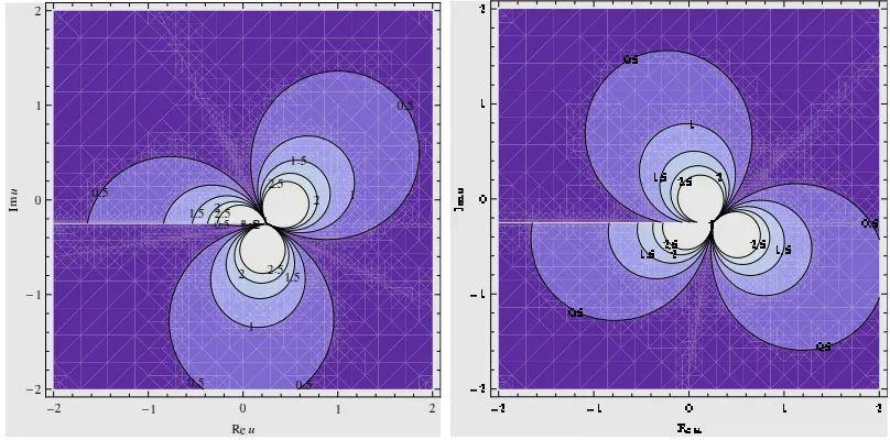
In figure 13 we show the first two members of the sequel parameterizing the deformation parameter asε=₋n/(n+1) withn= 1,2, . . .We observe that the pictures resemble flowers with 4 + 6n petals. We may predict the number of petals analytically as they are equal to the number of ζ₀ = 0 solutions computable by (3.9). For instance for the case n = 3 the formula (3.9) predicts the 16 valuesθ0 = (2ℓ−1)π/16 for the parameter choice c= 1,

β = 2 and γ = 3 with ℓ= 1, . . . ,16. We recognize these values in figure 13b. Note that the wedge regions separate different solutions from each other as the pointA is always an asymptotic fixed point.

Figure 13: Complex PT-symmetric rational solutions of the deformed KdV equation with A= 1/2, c= 1,β= 2 and γ= 3 for (a) H+₋1/2and (b)H

+

−2/3.

The trajectories appear to be qualitatively quite different for negative integer values of ε. For instance in figure 14a and 14b we depict some trajectories for the models with

Figure 14:ComplexPT-symmetric rational solutions of the deformed KdV equation withA= 1/2, c= 1,β= 2 and γ= 3 for (a) H+−2 and (b)H

+

−3.

For positive rational values of ε a complete trajectory extends over several different Riemann sheets. Figure 15a and 15b show the solutions ζ(1) and ζ(2), respectively. The angles for the ζ₀ = 0 solutions are predicted correctly by (3.9) to be θ0 = 4ℓπ/5 for

ℓ = 1, . . . ,5. A closed trajectory is obtained when passing the branch cut at_−∞ to 1/2 from the upper half plane in panel (a) to the lower half plane in panel (b). In figure 17a a single trajectory is depicted for Imζ₀= 1.

Figure 15: PT-symmetric rational solutions for H+1/3 : Different Riemann sheets for A = 1/2,

c= 1,β= 2 and γ= 3 (a) ζ(1) and (b)ζ(2).

is illustrated in figure 17b, where we depict just one single trajectory for Imζ₀ = 1. The trajectories for the _PT-symmetric and broken_PT-symmetric case look qualitatively very similar, the major difference being that the fixed point has moved away from the real axis, thus leading to a loss of the symmetry.

Figure 16: Broken PT-symmetric rational solutions for H1+/3 : Different Riemann sheets for

A= (1−i)/4,c= 1,β= 2 + 2iandγ= 3 (a)ζ(1) and (b)ζ(2).

Figure 17: Single trajectory for the rational solution ofH+1/3 with Imζ0= 1 : (a)PT-symmetric

solutions for the values as specified in figure 15, (b) BrokenPT-symmetric solutions for the values as specified in figure 16.

Figure 18: Single trajectory for the rational solution for ofH+3 with Imζ0= 1: (a)PT-symmetric

solutions for A = 1/2, c = 1, β = 2 and γ = 3, (b) BrokenPT-symmetric solutions for A = 1/4(1−i),c= 1,β= 2 + 2iandγ= 3.

another type of characteristics as more and more branches have to be taken into account for increasingε. In figure 18 and 19 we depict all branches for the trajectory with Imζ₀ = 1 forε= 3 and ε= 6, respectively.

Figure 19: Single trajectory for the rational solution for ofH+6 with Imζ0= 1: (a)PT-symmetric

solutions for A = 1/2, c = 1, β = 2 and γ = 3, (b) BrokenPT-symmetric solutions for A = 1/4(1−i),c= 1,β= 2 + 2iandγ= 3.

distort the trajectories, giving rise to new directions of the asymptotes, but not changing their numbers.

3.1.2 Trigonometric/hyperbolic solutions

As in the non-deformed case we assume next the factorization P(u) = (u₋A)2(u₋B), which will impose once more the constraints (2.14). Also in this case we can compute (3.5) numerically.

Again we supplement our numerical findings by some analytical results. We can predict once more the lines for which ζ₀ = 0 explicitly following the arguments of the previous subsection, with the difference that we have to take the limit to either the point A or B. For the angle of lines near the point Awe find

θ(_An,m,±)= π

2(ε₋1)[1−ε+ 4(n−m)−4mε] + 1

ε₋1arg(A−B) + 1

ε₋2arg(±λε) (3.10) whereas for the angle of lines near the pointB we compute

θ(_Bn,m,±)= π

2(ε−1−4n) + (1 +ε)2πm+ (ε−1) arg(B−A)−arg(±λε). (3.11) We depict some specific examples with different characteristics in the figures 20 to 24.

Figure 20: ComplexPT-symmetric trigonometric/hyperbolic solutions of the deformed KdV equa-tion withA= 4, B= 2, c= 1,β= 2 and γ= 3 for (a)H₋+1/2and (b)H

+

−2/3.

Figure 21: Single trajectory for the complexPT-symmetric trigonometric/hyperbolic solutions of the deformed KdV equation for H₋+1/2 with the same values as specified in figure 20 for (a)

Imζ0= 1 and (b) Imζ0=−1.

Figure 22: BrokenPT-symmetric trigonometric/hyperbolic solutions of the deformed KdV equa-tionH₋+1/2: (a) Spontaneously brokenPT-symmetry withA= 4 +i,B= 2−2i,c= 1,β = 3/10

andγ= 3; (b) brokenPT-symmetry withA= 4,B= 2,c= 1,β= 3/10 andγ= 3 +i.

−n/(n+ 1) with n = 1,2, . . . Notice also that unlike as in the case ε = 1 there is no distinction between a periodic and an asymptotically constant solution.

observe a connected trajectory in the two light shaded wedge region to the left of the vertical as can also be seen in figure 21. Such type of trajectories do not exist in the broken case as we can observe in figure 22. We note that instead trajectories from the light shaded region in the upper half plane connect to a dark shaded region in the lower half plane to the left of the corresponding light shaded region in the unbroken case.

Figure 23: ComplexPT-symmetric trigonometric/hyperbolic solutions of the deformed KdV equa-tion withA= 4,c= 1,β = 2 andγ= 3 for (a)H+−2 and (b)H

+

−3.

Figure 24: BrokenPT-symmetric trigonometric/hyperbolic solutions of the deformed KdV equa-tion forH+−2: (a) Spontaneously brokenPT-symmetry withA= 4 +i/2, B= 2−i, c= 1,β= 3/10

andγ= 3; (b) brokenPT-symmetry withA= 4, B= 2, c= 1,β= 3/10 andγ= 3 + 4i.

Comparing next the solutions for ε_∈R− _{we observe in figure 23a a similar}

Again we find that the rational solution resembles this solution for the same values of the deformation parameters, with the difference that the characteristic behaviour around the point Ain the rational case has been distorted to the points A andB.

The broken _PT-symmetric case for this model is presented in figure 24. In panel (a) we depict the spontaneously broken _PT-symmetric scenario for _H−+₂, observing that the symmetry is lost since the trajectories rotate together with the two fixed points. The_PT -symmetry is completely broken in the presentation in 24b for the same model. Having kept the values for the fixed points, we note that in this case the orbits rotate around them.

We have investigated also other models observing similar patterns, which we will how-ever not present here.

3.1.3 Elliptic solutions

-4 -3 -2 -1 -1 -1 0 0 0 0 1 1 1 1 2 2 2 2 3 3 3 3 4 4 4 4

-4 -2 0 2 4 6 8

-4 -2 0 2 4 Re u Im

u -3-2

-1 -1 -1 0 0 0 0 1 1 1 1 2 2 2 2 3 3 3 3 4 4 4 4

-4 -2 0 2 4 6 8

-4 -2 0 2 4 Re u Im u -1.5 -1 -1 -1 -0.5 -0.5 -0.5 0 0 0 0 0.5 0.5 0.5 0.5 1 1 1 1 1.5 1.5 1.5 2 2 2

-4 -2 0 2 4 6 8

-4 -2 0 2 4 Re u Im u

Figure 25: Elliptic solutions forH+−2: (a)PT-symmetric with A= 1, B = 3, C = 6, β = 3/10,

γ = −3 and c = 1; (b) spontaneously broken PT-symmetry with A = 1 +i, B = 3−i, C = 6, β = 3/10, γ = −3 and c = 1; (c) broken PT-symmetry with A = 1, B = 3, C = 6, β = 3/10, γ=−3 + 4iand c= 1.

Figure 26: Elliptic solutions for H+₋1/2: (a)PT-symmetric withA= 1,B = 3,C= 6,β = 3/10,

Proceeding just as in the undeformed case we specify nextP(u) = (u₋A)(u₋B)(u₋C), which imposes the constraints (2.22) and (2.23), thus leaving two constants free. We present here only the results for the cases ε=₋2 and ε=₋1/2 in the figures 25 and 26, respectively.

In all three possible scenarios we observe a similar qualitative behaviour as for the trigonometric/hyperbolic solutions of the previous subsection with the difference that we have three instead of two fixed points.

3.2 The _H−

ε-models

Let us now turn to the second type of deformation. In order to construct the solutions we proceed in a similar manner as in the previous case. Integrating now twice the second equation in equation (3.3) we obtain

u2_ζ = 2

γ

κ2+κ1u+

c

2u

2_−β iε

(1 +ε)(2 +ε)u

2+ε

=:λQ(u), (3.12)

where

λ=₋ 2βi

ε

γ(1 +ε)(2 +ε). (3.13)

A crucial difference between_H+

ε andH−ε is that unlike as the polynomialP(u), which was

of fixed order 3, the order of Q(u) depends on ε, meaning that we have more and more possibilities to factorize it for growingε. For instance, for a given integer valuen_∈N_{0 the}

factorization of Q(u) as

Q(u) = (u₋A1)ε+2−n

Yn

i=1(u−Ai+1), (3.14)

admits solutions provided n₋2 _≤ ε _≤ n+ 1 and ε _∈ N_{. This allows of course for yet}

another infinity of possibilities.

When κ1 = κ2 = 0 we can find a closed solution valid for all ε by integrating (3.12) and solving it foru

u(ζ) =





c(ε+ 1)(ε+ 2)

iε_βh_cosh√cε_√(ζ−ζ0)

γ

+ 1i





1/ε

. (3.15)

The generic scenario does not yield such a simple answer.

3.2.1 _H−₂

This case is especially interesting as it corresponds to a complex version of the modified KdV-equation. Specifying (3.14) for instance asQ(u) = (u₋A)3(u₋B) we can factorize the polynomial in (3.12) with the choice

κ1=− 2c3/2

3√₋β, κ2 =− c2

4β, A=− B

3 and B =−

3√c √

−β. (3.16)

Notice that this fixes all the boundary conditions for a given model. Solving (3.12) then yields a rational solution for the second equation in (3.3)

u(ζ) =

r

−c β

2cζ2₋9γ

As is well know for the real case one may construct solutions for the KdV-equation from those of the modified KdV-equation by means of a Miura transformation. We expect this also to hold for their complex versions. Indeed, using the transformation of the form

uKdV(ζ) =

r

6γ β uζ−u

2 _(3.18)

yields the rational solution of the KdV-equations (2.12) from (3.17) when we identify

ζ₀ =ip

3γ/2c therein.

Assuming in (3.14) instead Q(u) = (u₋A)2(u ₋B)(u ₋C) we can factorize the polynomial in (3.12) with the constraints

κ1 =

βC2_{(ϑ−5Cβ) + 9c(ϑ−3Cβ)}

81β , κ2 =

C(2ϑ₋Cβ) (Cβ+ϑ)2

324β2 , (3.19)

A = ₋1

2(B+C) and B =

2ϑ₋Cβ

3β (3.20)

where we abbreviated ϑ := √2p

−β(βC2_{+ 9c). Notice that in this case one constant} remains free. The integration of (3.12) yields in this case a trigonometric solution, which, using the same Miura transformation (3.18), may also be converted into a solution of the KdV-equations.

3.2.2 _H−₄

In this case the polynomial of the right hand side of (3.12) is of sixth order. We present here just one very symmetric solution by assuming a factorization of the form Q(u) =

u2(u2₋B2)(u2₋C2), which is possible with the simple choice

κ1 =κ2 = 0, B=iC and C4= 15c

β . (3.21)

Thus we have made contact with the solution (3.15). Parameterizing B = rBeiθB and

λ=rλeiθλthe eigenvalues of the Jacobian when linearized aboutu= 0 are easily computed

to

j1 =±i√rλrB2 exp

i

2(4θB+θλ)

and j2 =∓i√rλrB2 exp

−₂i(4θB+θλ)

. (3.22)

This means for the_PT-symmetric solution we always obtain two real degenerate eigenvalues and therefore a star node at u = 0. For the positive square root in (3.12) with B =

±(15c/β)1/4 or with B = _±i(15c/β)1/4 the node is stable or unstable, respectively. The stability property is reversed for the negative square root. Taking the branch cuts at Imu = 0, Reu= 0, Imu= Reu and Imu=₋Reu into account we obtain closed curves. The four zeros ofQ(u), i.e. _±(15c/β)1/4,_±i(15c/β)1/4, are surrounded by the trajectories. All these features can be seen in figure 27a. We may also tune the coupling constants in such a way that 4θB+θλ = 0, which by (3.22) implies that the fixed point at the origin

Figure 27: PT-symmetric solutions forH−

4 : (a) Star node at the origin forc = 1,β = 2, γ= 1

andB= (15/2)1/4_{; (b) centre at the origin forc= 1,β = 1,γ=−1 andB = (15/2)}1/4_.

Figure 28: BrokenPT-symmetric solution forH−

4: (a) Star node at the origin forc= 1,β = 2+i3,

γ = 1 and B = (15/2 +i3)1/4_{; (b) centre at the origin for c = 1, β = 2 +i3, γ = −1 and}

B= (30/13−i45/13)1/4_.

Since we have no free parameter left in our factorization this solution can not be broken spontaneously. A complete breaking is carried out by complexifyingβ orγ. When choosing Imβ ₆= 0 we can still achieve in (3.22) that 4θB+θλ =±π, such that the star node nature of

the fixed point is preserved despite the fact that the_PT-symmetry is lost. For a particular choice this behaviour is depicted in figure 28a. More surprising is the fact that we can also achieve that 4θB+θλ = 0 in the broken case. This means the eigenvalues in (3.22) are

case.

In contrast for Imγ ₆= 0 the eigenvalues ji will become complex and the fixed point

at the origin turns into an unstable or stable focus. Taking the branch cut structure into account we observed this behaviour in figure 29a for β _∈ R_{, γ ∈} C _{and in figure 29b for}

β _∈C_{,γ ∈}C_.

-3 -2 -1 0 1 2 3

-3 -2 -1 0 1 2 3

Re u

Im

u

Figure 29: Broken PT-symmetric solution for H−

4: (a) focus at the origin for c = 1, β = 2,

γ= 1 +i3 andB = (15/2)1/4_{; (b) focus at the origin for Imζ}

0= 0.8,c= 1,β= 2 +i3,γ=−1 +i2

andB= (30/13−i45/13)1/4_.

Once again we observed that when identifying a coupling constant as a bifurcation parameter, the origin undergoes a Hopf bifurcation.

Making once more the identificationu_→xand ζ _→tfor our traveling wave equation together with the identification

κ1 = 0, κ2 =γE, and β=γg(1 +ε)(2 +ε) (3.23)

equation (3.12) converts into the classical deformation of the harmonic oscillator

H=E = 1 2p

2

−₂c_γx2+gx2(ix)ε. (3.24)

Setting furthermorec= 0, which in our setting corresponds to a static solution, we obtain precisely the potential treated in the seminal paper by Bender and Boettcher [4].

4. Complex coupled nonlinear wave equation of Ito type

the second fieldv(x, t) and the assumption of a specific form of the evolution equation for this field. The coupled system describing this type of scenario acquires the general form

ut+αvvx+βuux+γuxxx = 0, α, β, γ∈C, (4.1)

vt+δ(uv)x+φvxxx = 0, δ, φ∈C. (4.2)

Imposing the constraints β = 3γ, φ = 1, δ = 3 on the constants and leaving α, γ free, the Hirota method can be applied to establish that the system (4.1) and (4.2) possesses N-soliton solutions [40]. When selecting in addition γ = ₋1/2 as in [41] or α = ₋2,

β =₋6, γ = ₋1, δ = ₋2 and φ= 0 as in [42], it was established in both cases that the system possesses infinitely many charges. Forφ= 0 the system (4.1) and (4.2) was shown to possess soliton solutions of cusp type [43]. Notice also that when complexifying the KdV-field in (2.2) as uKdV → u+iv we obtain the system (4.1) and (4.2) for the special choiceα=₋β_KdV,β =β_KdV,γ =γ_KdV,δ=β_KdVand φ=γ_KdV. In the following we will mainly discuss the case φ = 0, such that even the real case of (4.1) and (4.2) is distinct from the complexified version of the KdV equation.

It is straightforward to verify that for the choice δ =α the system of equations (4.1) and (4.2) results from a variation of a Hamiltonian whose density is given by

HI =−

α

2uv 2

−β₆u3+γ 2u

2

x+

φ

2v 2

x, (4.3)

when using the variational derivative and time evolution in the standard way

wt=

∂ ∂x

X∞

n=0(−1)

n dn

dxn

∂_HI

∂wnx

x

for w=u, v. (4.4)

The Hamiltonian resulting from the density (4.3) is manifestly_PT-symmetric as it remains invariant under a simultaneous parity transformation and time reversal which may be realised in four alternative ways as

PT++ : x7→ −x, t7→ −t, i7→ −i, u7→u, v 7→v forα, β, γ, φ∈R, (4.5)

PT+− : x7→ −x, t7→ −t, i7→ −i, u7→u, v 7→ −v forα, β, γ, φ∈R, (4.6) PT−+ : x7→ −x, t7→ −t, i7→ −i, u7→ −u, v7→v foriα, iβ, γ, φ∈R, (4.7)

PT−− : x7→ −x, t7→ −t, i7→ −i, u7→ −u, v7→ −v foriα, iβ, γ, φ∈R, (4.8)

depending on whether we choose the fieldsu, vto be_PT-symmetric or anti-symmetric. All possibilities ensure that _PTij :HI 7→ HI holds withi, j ∈ {+,−}. First we will exploit

these possibilities to explain the reality of the energies and in section 5 we use them to define new physically feasible models.

4.1 _PT-symmetric, spontaneously broken and broken solutions

As usual in this context we assume that the fields acquire the form of a traveling wave

u(x, t) = u(ζ) and v(x, t) = v(ζ) with ζ = x₋ct. In [44] it was shown for the case

inconsistent. We extrapolate here without rigorous proof that this assumption can be made without loss of generality even in other cases. Let us briefly recall how these equations may be solved in a systematic way. To begin with we integrate (4.1) and (4.2) to

−cu+ α 2v

2₊β

2u

2_+γu

ζζ = κ1, (4.9)

−cv+αuv = κ2, (4.10)

with integration constants κ1, κ2. In the following we always exclude the case κ2 = 0 as this implies the vanishing of the new fieldv= 0, which means a reduction to the deformed KdV equation, or a constant KdV-field u=α/c. Multiplying (4.9) by uζ, using (4.10) to

replace vby u in (4.9), we can integrate once more and obtain

u2_ζ = 2

γ

κ3+κ1u+

c

2u 2

−β₆u3+κ 2 2 2

1

αu₋c

. (4.11)

This equation is difficult to solve directly, but following [43] we trade theu field for thev

field with

u= c

α + κ2

αv and uζ=− κ2

αv2vζ (4.12)

and obtain

v_ζ2=₋ v 3αγκ2₂

4

X

k=0

akvk, (4.13)

where

a0 =βκ32, a1= 3cκ22(β−α), a2 = 3κ2(βc2−2αc2−2α2κ1),

a3 =c3(β−3α)−6α2(cκ1+ακ3), a4 =−3α3κ2.

(4.14)

At first sight this looks even less encouraging than (4.11). However, now the right hand side is a polynomial and in case we can factorize the sumP4

k=0akvk into some convenient

form we may be able to integrate (4.13) similarly as in the previous section. Up to one integration the solution is therefore

±√λ(ζ₋ζ₀) =

Z

dv p1

R(v), (4.15)

withλ=α2/γκ2 and λR(v) corresponding to the right hand side of (4.13). We note that not all conceivable assumptions for the sum will lead to meaningful or nontrivial solutions. Taking for instance R(v) = v4(A+v) or R(v) = v3(A+v)(B +v) with some unknown constantsA andB leads in both cases to κ2 = 0 orβ = 0, which we exclude for the above mentioned reasons.

When demanding vanishing asymptotic boundary conditions for the u-field and its derivatives, the relations (4.9) and (4.11) imply that we satisfy the additional constraints

lim

ζ→±∞u, uζ, uζζ = 0 ⇒ κ1 = ακ2

2

2c2 , κ3=

κ2 2

2c, ζ→±∞lim v=− κ2