A Method for detection and quantification of building damage using post-disaster LiDAR data

Rochester Institute of Technology

RIT Scholar Works

Theses Thesis/Dissertation Collections

8-4-2011

A Method for detection and quantification of

building damage using post-disaster LiDAR data

Richard Labiak

Follow this and additional works at:http://scholarworks.rit.edu/theses

This Thesis is brought to you for free and open access by the Thesis/Dissertation Collections at RIT Scholar Works. It has been accepted for inclusion

in Theses by an authorized administrator of RIT Scholar Works. For more information, please [email protected].

Recommended Citation

A METHOD FOR DETECTION AND QUANTIFICATION OF BUILDING DAMAGE USING POST-DISASTER LIDAR DATA

by

Richard C. Labiak

Bachelor of Science, Electrical Engineering

United States Air Force Academy, 2006

A thesis submitted in partial fulfillment of the

requirements for the degree of Master of Science

in the Chester F. Carlson Center for Imaging Science

Rochester Institute of Technology

August 4, 2011

Signature of the Author____________________________________________

CHESTER F. CARLSON CENTER FOR IMAGING SCIENCE

ROCHESTER INSTITUTE OF TECHNOLOGY

ROCHESTER, NEW YORK

CERTIFICATE OF APPROVAL

M.S. DEGREE THESIS

The M.S. Degree Thesis of Richard C. Labiak has been examined and approved by the

thesis committee as satisfactory for the thesis requirement for the M.S. degree in Imaging Science

_____________________________________ Dr. Jan A.N. van Aardt, Thesis Advisor

_____________________________________ Dr. David W. Messinger

_____________________________________ Dr. Harvey E. Rhody

_____________________________________ Date

THESIS RELEASE PERMISSION

CHESTER F. CARLSON CENTER FOR IMAGING SCIENCE

ROCHESTER INSTITUTE OF TECHNOLOGY

Title of Thesis:

A Method for Detection and Quantification of Building Damage Using Post-Disaster LiDAR Data

I, Richard C. Labiak, hereby grant permission to the Rochester Institute of Technology to reproduce my print thesis or dissertation in whole or in part. Any reproduction will not be for commercial use or profit.

Abstract

There is a growing need for rapid and accurate damage assessment following natural disasters, terrorist attacks, and other crisis situations. The use of light detection and ranging (LiDAR) data to detect and quantify building damage following a natural disaster was investigated in this research. Using LiDAR data collected by the Rochester Institute of Technology (RIT) just days after the January 12, 2010 Haiti earthquake, a set of processes was developed for extracting buildings in urban environments and assessing structural damage. Building points were separated from the rest of the point cloud using a combination of point classification techniques involving height, intensity, and multiple return information, as well as thresholding and morphological filtering operations. Damage was detected by measuring the deviation between building roof points and dominant planes found using a normal vector and height variance approach. The devised algorithms were incorporated into a Matlab graphical user interface (GUI), which guided the workflow and allowed for user interaction. The semi-autonomous tool ingests a discrete-return LiDAR point cloud of a post-disaster scene, and outputs a building damage map highlighting damaged and collapsed buildings.

Acknowledgments

This thesis would not have been possible without the help and support of many

individuals. First and foremost, I would like to thank my advisor, Dr. Jan van Aardt, for

guiding me through this process and always having my best interests in mind. He

challenged me to think critically and taught me to be confident in my work. Thank you

Jan for being so responsive and always having the time to meet with me. I would also

like to thank my other committee members, Dr. David Messinger and Dr. Harvey Rhody,

for helping me stay on track and for providing valuable insight.

This project required understanding and access to the data collected during the

Haiti campaign. To this end, Jason Faulring and Steve Cavilia were invaluable resources

and I really appreciate all of their help. I would also like to thank Don McKeown for

providing the EEFIT truth data, and Cindy Schultz for all of her administrative support. I

would like to acknowledge all of my Imaging Science instructors, for not only giving me

the knowledge base to complete this research, but also for developing my interest in the

field. A special thanks goes out to my fellow Air Force and LiDAR students, who have

been great officemates and friends.

Finally, I would like to thank my parents and close friends. I truly appreciate the

constant support you guys have given me throughout the past two years. Thanks for

being so patient with me, and know that your encouragement and love did not go

Table of Contents

Page

Abstract...iv  

Acknowledgments ...v  

Table of Contents...vi  

List of Figures... viii  

1   Introduction...1  

2   Project Overview ...6  

2.1   Research Questions ...6  

2.2   Objectives...6  

3   Background...9  

3.1   Chapter Overview ...9  

3.2   Light Detection and Ranging (LiDAR) Remote Sensing Systems ...9  

3.3   LiDAR Technology in Disaster Management...12  

3.4   Digital Terrain Model (DTM) Extraction from a LiDAR Point Cloud...15  

3.5   Building Detection from LiDAR Point Cloud ...19  

3.6   Recognizing Damaged Buildings in LiDAR Data ...26  

3.7   Chapter Summary...27  

4   Methodology...29  

4.1   Chapter Overview ...29  

4.2   World Bank/ImageCat Inc./RIT Haiti Earthquake Dataset...29  

4.3   LiDAR Point Cloud Preprocessing ...33  

4.4   Building Segmentation...41  

4.6   Validation ...71  

4.7   Chapter Summary...75  

5   Results and Discussion ...76  

5.1   Chapter Overview ...76  

5.2   Building Segmentation Performance ...76  

5.3   Building Damage Detection Performance...87  

5.4   Chapter Summary...97  

6   Conclusion ...99  

References...103  

Appendix A...109  

A.1   Validation Sites ...109  

A.2   Building Segmentation Results – Output Building Maps ...109  

A.3   Damage Detection Results ...112  

Appendix B...117  

B.1   Matlab GUI Screenshots ...117  

List of Figures

Figure Page

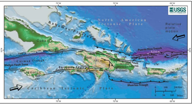
Figure 1. Topographic map showing the northern Caribbean plate boundary. The January

12, 2010 Haiti earthquake, marked by a star, occurred along the Enriquillo Fault

(Eberhard et al., 2010). ...2  

Figure 2. Logistical challenges presented relief workers with a difficult task. Above:

Toussaint Louverture International Airport in Port-au-Prince with one runway and a

small cargo ramp. Below: The main seaport in Port-au-Prince was closed after the

docks, a gantry crane, and some shipping containers collapsed into the water

(Wildfire Airborne Sensing Program (WASP) imagery)...2  

Figure 3. Example GEO-CAN damage assessment map of Port-au-Prince. The buildings

outlined in red were manually classified as being damaged by a network of over 600

skilled volunteers (Eberhard et al., 2010)...5  

Figure 4. Map showing damage assessment and location and condition of field hospital

sites in Port-au-Prince. The data are current as of January 26, 2010, two weeks

following the magnitude 7.0 earthquake (ReliefWeb, 2010)...5  

Figure 5. LiDAR instrument mounted to a fixed-wing aircraft. Combining the range, scan

angle, laser position from GPS, and laser orientation from INS, accurate X, Y, Z

ground coordinates can be calculated for each laser pulse (Lohani, 2010). ...11  

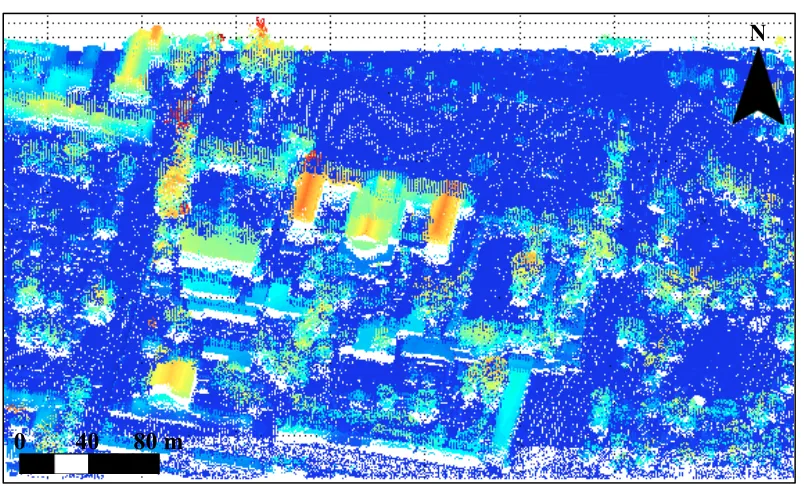
Figure 6. LiDAR point cloud of Haiti's Presidential Palace and surrounding area. The

The ground points are shown in royal blue, while the highest points are displayed in

red. ...11  

Figure 7. Nadir view of the point cloud of Haiti's Presidential Palace and surrounding

area colored to show different information. Top Left: Height image with ground

points shown in royal blue and the highest points in red. Top Right: Intensity image

with white representing high intensity or the most reflective objects, and black

representing low intensity. Bottom: Multiple return image displaying non-first return

points in red...13  

Figure 8. One-dimensional view of TIN ground surface adapting to LiDAR points. Note

how well the surface is approximated from below, despite the intermittent gaps

caused by buildings (Axelsson, 2000). ...18  

Figure 9. Catalog of different damage types of buildings occurring after earthquakes

(Schweier and Markus, 2004). ...28  

Figure 10. Comprehensive flowchart showing the workflow broken down into three

distinct tasks: Preprocessing, building segmentation, and damage detection. Dotted

lines represent links between tasks, as inputs needed for certain processes come from

earlier stages of the workflow...30  

Figure 11. Main menu of the Matlab-based LiDAR Building Damage Detection Tool. ..31  

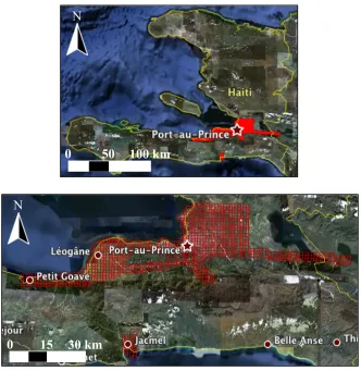
Figure 12. Above: Map of Haiti showing the data collection region in red. Below:

Zoom-in view of the area affected by the earthquake. Each 1 km x 1 km tile outlZoom-ined Zoom-in red

represents an individual LAS file containing on average 3 to 5 million LiDAR points

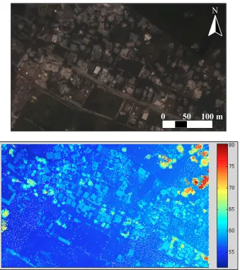
Figure 13. Scene captured over the city of Darbonne on January 25, 2010. Above: WASP

image with a spatial resolution of 0.15 m. Below: Corresponding raw LiDAR point

cloud colored by elevation. Point heights in the scene range from 51 m to 80 m,

before the effect of terrain is considered...33  

Figure 14. Angle and distance parameters must be met every iteration for a point to be

added to the ground surface model. The iteration angle is defined at the maximum

angle between a point, its projection on the triangle surface, and the closest triangle

vertex. The iteration distance is defined as the maximum distance from a point to the

triangle surface (TerraScan, 2011)...36  

Figure 15. One-meter resolution Digital Terrain Model (DTM) of the region surrounding

Haiti’s National Palace. The colored mesh represents the ground surface

approximation, and the black points are the vendor-classified ground points. Above:

Oblique view with a stretched z-axis to show elevation change. Below: Nadir view.

...39  

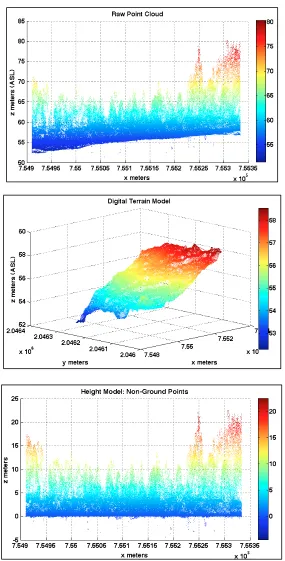
Figure 16. The effect of the terrain is eliminated from the point cloud of the city of

Darbonne. The points are colored by elevation according to the colormap for each

plot. Top: Raw point cloud prior to DTM extraction. Middle: DTM approximated

using natural neighbor interpolation of the ground points. Bottom: Height model

created by subtracting the height of the terrain from each non-ground point...40  

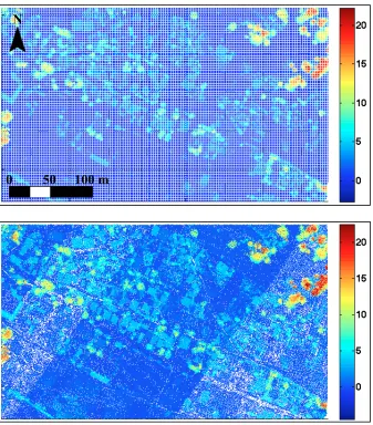
Figure 17. Height models of Darbonne created using two different techniques. Above:

model. Below: Point-based height model created by subtracting the corresponding

DTM height from non-ground points. ...41  

Figure 18. Two prominent building construction types found in Haiti. Above: Shanty

housing made of wood and a corrugated metal roof. Below: Residential buildings

constructed of reinforced concrete columns, infill concrete walls, and concrete slab

floors and roofs (Eberhard et al., 2010)...43  

Figure 19. Normalized intensity metric used to identify building regions. Building

regions are assumed to have uniform intensity, so building pixel values should be

close to one. Left: Haiti's National Palace and surrounding area. Right: The Darbonne

area...44  

Figure 20. Vegetation points are removed from the raw point cloud by finding points with

high height variance. The tile resolution used was 2 m x 2 m, resulting in

approximately 14 points per tile. ...46  

Figure 21. Binary masks with the tiles flagged for removal shown in black. Above: Mask

created by assigning a value of one to high height variance tiles (black). Below: Mask

after applying a Gaussian lowpass filter with a 2 x 2 kernel. ...47  

Figure 22. Raw point cloud with additional vegetation tiles removed as a result of

Gaussian lowpass filtering. ...47  

Figure 23. A profile view of the Darbonne point cloud used to determine the best height

threshold...51  

Figure 25. The LiDAR point cloud, referenced above ground, with points below 2 m

removed...51  

Figure 26. Images portraying different metrics that can be used for building

segmentation. Top to bottom: normalized height, normalized intensity, maximum

height, and multiple returns. ...52  

Figure 27. Normalized height image with pixel values less than 0.9 removed. ...53  

Figure 28. Result of using a Gaussian lowpass filter, with a 2 x 2 kernel, on the image in

Figure 27. ...53  

Figure 29. Result of applying a normalized height threshold of 0.8 to Figure 28...53  

Figure 30. Binary multiple return mask created by applying a Gaussian lowpass filter to

the multiple return image. Black pixels correspond to areas with more than one

multiple return, which is indicative of vegetation. ...54  

Figure 31. Result of masking out the areas with more than one multiple return from the

initial building map in Figure 29. ...54  

Figure 32. Building map after morphological opening using a two-pixel wide square

structuring element...56  

Figure 33. Final building map of Darbonne showing the 205 building regions detected.

Each unique building region is shown in a different color. ...56  

Figure 34. Point cloud of a building region, extracted from the Darbonne scene...58  

Figure 35. Histogram of the angles between the normal vector to every tile plane and a

Figure 36. Building point cloud with the normal vectors shown for each tile. The blue

vectors correspond to undamaged points, while the red vectors indicate damage.

According to the normal angle metric, 42% of the building points are damaged. ...60  

Figure 37. Histogram of the height variances of tiled points within a building region point

cloud. Of the 52 tiles, 33 have variances below the 0.03 threshold, shown in red. The

19 tiles with larger variances are likely to contain damaged points. ...62  

Figure 38. Building region point cloud with damaged points, as defined by the variance

metric, shown in red. According to the metric, 30% of the building points are

damaged. ...62  

Figure 39. The slopes between consecutive points can be used to detect damaged points.

In the set of points on the left, the slopes between points A and B and points B and C

are constant, so point B is undamaged. On the right, the slope between points A and

B is much steeper than the slope between points B and C, so in this case it is assumed

that point B is damaged...63  

Figure 40. Nadir view of a building region point cloud. The scan lines followed to

compute the slope differences are overlaid in the x direction (left) and y direction

(right). ...64  

Figure 41. Building region point cloud with damaged points, as defined by the line-based

slope difference metric, shown in red. According to the metric, 22% of the building

points are damaged. ...64  

Figure 42. Plots comparing combinations of the three damage detection metrics. The

Figure 43. Plots comparing combinations of the three damage detection metrics. The

points represent building truth from the scene surrounding Haiti’s National Palace. 67  

Figure 44. Building damage maps of the scene surrounding Haiti’s National Palace (left)

and Darbonne (right). GEO-CAN assessments in this scene range from Grade 1

(undamaged) to Grade 5 (destroyed). ...69  

Figure 45. Example damage assessment maps that could be given to emergency managers

or responders on the ground following a disaster. The buildings assessed to be highly

damaged are shown in red, while building in black are assumed to be undamaged...70  

Figure 46. Slope map in degrees of the Darbonne terrain calculated by ArcMap. The

average slope of the scene is 1.66°, so the terrain would be considered “flat”. ...73  

Figure 47. Image of the Turgeau validation site located in Southeast Port-au-Prince. The

blue dots correspond to GEO-CAN damage assessments, while the yellow dots

represent EEFIT evaluations...74  

Figure 48. Truth building outlines for the National Palace validation site are overlaid on

the output building map (left) and WASP imagery (right). Haiti’s Bicentennial

Monument, located in the top-right corner of the scene, was the only building not

detected. The normalized height and normalized intensity metrics that are used to

classify building points and look for uniform point areas, were hampered by the

monument’s tall and very steep sides. ...79  

Figure 49. Zoom-in area of the Darbonne validation site illustrating the effects of

over-segmentation. Arrows point to building segments in the output building map (left)

by the thick vegetation that was not completely removed during the building

segmentation process. ...79  

Figure 50. Zoom-in area of the Palace validation site where over-segmentation of a long

building has resulted in two separate building regions. Close examination of the

WASP image (right) shows that the building was heavily damaged from the

earthquake, which influenced the segmentation results...80  

Figure 51. Section of the Palace validation site showing poor segmentation results for an

area with a high concentration of buildings. All of the buildings were detected but the

segments do not accurately represent the actual buildings. ...81  

Figure 52. Truth building outlines for the Léogâne validation site are overlaid on the

output building map (left) and WASP imagery (right). Though 24 of the buildings

were detected, the segmentation results do not characterize the size, shape, and

orientation of the actual buildings in the scene...82  

Figure 53. Zoom-in area of the Riviere Froide validation site. Over 20 buildings exist in

this 50 m x 70 m area, but were too small and dense to be properly segmented...83  

Figure 54. Truth building outlines for the Grand Goave validation site are overlaid on the

output building map (left) and WASP imagery (right). Notice that many of the small

building regions, typically those less than 5 m x 5 m in size, went undetected by the

building segmentation routine...84  

Figure 55. Zoom-in area of Grand Goave showing five small buildings that went

m wide, too small to survive the filtering and morphological operations that were

used as part of the segmentation. ...84  

Figure 56. Truth building outlines for the Darbonne validation site are overlaid on the

output building map (top) and WASP imagery (bottom). Ten of the 30 truth buildings

went undetected in this scene, primarily due to small building size and questionable

truth data. ...86  

Figure 57. Zoom-in area of the Darbonne site showing three questionable building

regions that were all given GEO-CAN damage assessments. The two areas indicated

by yellow arrows were incorrectly included in the truth data set. Google Earth

imagery (right) was useful in discerning actual buildings from bare earth and

livestock corrals. ...86  

Figure 58. Some ground points are included in the building point cloud due to small

geometric registration errors between the LiDAR height model and the WASP

imagery, used to trace the building outline. The extra ground points affected the

overall damage percentage, but not enough in this case for the algorithm to

incorrectly classify the building as damaged. ...90  

Figure 59. Building located in the Riviere Froide validation site whose outline was not

traced accurately. This caused many tree points, ground points, and points from

adjacent buildings to be included in the building point cloud. As a result, the

algorithm detected enough damage to misclassify the building as Damage Grade 3-5.

Figure 60. The damage detection routine incorrectly identified damage along all the roof

joints due to the way the points were tiled. The truth undamaged building was

determined to be 66% damaged (classified into Damage Grade 3-5). ...92  

Figure 61. The major damage in this building from the Grand Goave validation site was

detected, but it was not enough to classify the building as damaged. This was the

only building in the Grand Goave site that was under-classified. ...92  

Figure 62. The damage detection routine did not recognize the smaller building plane and

therefore classified all the points on that plane as damaged. The entire building was

assessed to be 59% damaged and ended up being misclassified as Damage Grade 3-5.

The building was rated Damage Grade 1 by the GEO-CAN effort...93  

Figure 63. Léogâne building that was rated Damage Grade 3 by GEO-CAN, but was

classified as undamaged by the damage detection routine. The LiDAR building point

cloud (left), WASP image (middle), and Google Earth image (right) appear to

confirm the results of the routine. ...94  

Figure 64. Partially collapsed building in the Turgeau validation site that was classified as

Damage Grade 1 by the damage detection routine. The concrete roof slab remained

intact, which caused the algorithm to assume it was undamaged...95  

Figure 65. Building in the Turgeau validation site that appeared undamaged and was

classified as Damage Grade 1 by the damage detection algorithm. Based on ground

observations, EEFIT assessed the building at Damage Grade 3. This level and

Figure 66. The damage detection routine calculated the percent damage for this building

to be 50%, just shy of the 51% threshold for classifying a building as damaged...96  

Figure 67. Collapsed Grade 5 building in the Palace validation site that was calculated to

be 100% damaged. ...97  

Figure 68. The damage detection algorithm performed well on the Bicentennial

1 Introduction

On January 12, 2010 at 4:53 PM local time, a magnitude 7.0 MW earthquake

struck the Republic of Haiti. This natural disaster, one of the most destructive in history,

killed an estimated 230,000 people, injured 300,000, and displaced 1.6 million from their

damaged or destroyed homes (USAID, 2010). The epicenter of the earthquake was

located 25 km southwest of Port-au-Prince, Haiti’s largest city and densely populated

capital. At the time of the disaster, roughly 2 million people lived within the zone that

suffered heavy to moderate structural damage (CIA, 2011). According to the United

States Geological Survey (USGS), 97,294 houses were destroyed and 188,383 were

damaged in Port-au-Prince and in much of southern Haiti (USGSa, 2011). In the days

following the earthquake, individuals and organizations from around the world descended

upon Haiti to help search for survivors, provide food, water, medicine, and shelter, and

start the rebuilding effort.

Logistical challenges quickly surfaced as international humanitarian relief and

military aid poured into the Caribbean country. Toussaint Louverture International

Airport, Port-au-Prince’s only international airfield, had just a single runway, single

taxiway, and a small, crowded ramp (Jones, 2011). The city’s main seaport was closed

after severe damage to the docks and its one major gantry crane. In addition, many of the

roads were impassable, either directly damaged by the earthquake or blocked by rubble

(Davidson and Smith, 2011). The sheer scale of the disaster presented rescuers with a

seemingly overwhelming task, and a need quickly arose for the ability to provide timely

Figure 1. Topographic map showing the northern Caribbean plate boundary. The January 12, 2010

Haiti earthquake, marked by a star, occurred along the Enriquillo Fault (Eberhard et al., 2010).

Figure 2. Logistical challenges presented relief workers with a difficult task. Above: Toussaint

Louverture International Airport in Port-au-Prince with one runway and a small cargo ramp.

Below: The main seaport in Port-au-Prince was closed after the docks, a gantry crane, and some shipping containers collapsed into the water (Wildfire Airborne Sensing Program (WASP) imagery).

0 150 300 m

N

N

According to Ronald Eguchi, President and CEO of ImageCat, Inc., the Haiti

earthquake was one of the first events where remote sensing technology was “embraced

at such a large scale in a real operational sense” (Eguchi et al., 2010). Starting within

days of the disaster, vast amounts of high-resolution satellite and aerial optical imagery

and Light Detection and Ranging (LiDAR) data were collected on a daily basis.

ImageCat, the World Bank’s Global Facility for Disaster Reduction and Recovery

(GFDRR), the Rochester Institute of Technology (RIT), the Earthquake Engineering

Research Institute (EERI), and the Multidisciplinary Center for Earthquake Engineering

Research (MCEER) were among the organizations that used these data to guide damage

assessment and rescue and recovery efforts (Eberhard et al., 2010).

ImageCat, in partnership with many of the organizations listed above, formed a

worldwide network of engineers and scientists tasked with analyzing Haiti imagery and

performing damage assessment on more than 30,000 buildings. The Global Earth

Observation – Catastrophe Assessment Network (GEO-CAN), consisting of over 600

volunteers at its height, manually identified damaged buildings by comparing a

combination of 50 cm resolution Geo-Eye-1 imagery and 15 cm resolution Google and

Wildfire Airborne Sensing Program (WASP) imagery with imagery collected before the

disaster (Bevington et al., 2010). GEO-CAN officially started on January 21, 2010,

though thermal IR and LiDAR were not used until March 5, 2010, when the third phase

of the effort got underway to identify debris, liquefaction, and investigate thermal and

geological anomalies caused by the earthquake (EERI, 2010). An example GEO-CAN

In addition to the GEO-CAN campaign, the National Geospatial-Intelligence

Agency (NGA), the German Space Agency (DLR), Information Technology for

Humanitarian Assistance Cooperation and Action (ITHACA), and the United Nations

Operational Satellite Applications Program (UNOSAT) were among numerous other

agencies that either used or made available imagery to aid in recovery and rebuilding in

Haiti (Eberhard et al., 2010). Figure 4 shows a damage assessment product that

combines information from these agencies. The map not only highlights areas of

moderate to catastrophic damage in red, but it also displays the location and condition of

field medical sites (ReliefWeb, 2010).

Since the availability of high quality remote sensing data is no longer a limiting

factor in disaster response, focus is now being directed towards developing useful

information products that can be derived from the data. Eguchi states, “While the area of

remotely-sensed damage assessment took a quantum step forward in the Haiti campaign,

there is still significant room for improvement” (Eguchi et al., 2010). Much of the

damage assessment in Haiti took days to weeks to perform, mostly due to the intense and

manual nature of the work. The availability of a damage map produced in near real-time

would help satisfy the never-ending need to reduce the response phase in the disaster

management cycle. Creating a damage map within hours of a natural disaster is not a

trivial task, but this research details an effort using LiDAR technology and limited human

Figure 3. Example GEO-CAN damage assessment map of Port-au-Prince. The buildings outlined in red were manually classified as being damaged by a network of over 600 skilled volunteers

(Eberhard et al., 2010).

Figure 4. Map showing damage assessment and location and condition of field hospital sites in Port-au-Prince. The data are current as of January 26, 2010, two weeks following the magnitude 7.0 earthquake (ReliefWeb, 2010).

Trinity Norwegian Sanatorium Sacre Coeur Pere Damien Bernard Mevs MSF Hospital

Freres Rehab (unv) Asile Communal

Caritas Hospital

Hospital Francais

Hopital St. Esprit

St. Joseph Hospital

iti

Maternite Isaie Jeanty

Hospital Frances (unv) De Sante De Cathedrale

Red Cross Blood Bank

Hopital Le Messie (unv)

Sainte Catherine Laboure

Grace Childrens Hospital

Hospital of Peace (la Paix) National Reference Lab

Community Hospital of Haiti University Hospital of Haiti

Eliazer Germain Heath Center

Chinese Field Hospital (UNV)

St. Francois de Sales Hospital

Hospital Canape Vert Health Center of Portail Leogane

De L'Ofatma (Maternity Hospital)

Argentina Military Hospital/MINUSTAH

Centre de Psychiatrie/Neuropsychiatre

Hospital St. Charbel/Delmas Multimed 2

OFATMA

CLIMAPEV Hopital Espoir

Japanese BHC Unit

Brazilian Hospital Spanish Field Hospital/Belgian (unv)

Russian Field Hospital Israeli Field Hospital

Finnish BHC Unit Croix-Deprez Finnish BHC Unit - Place Jeremie

Italian Hospital and St. Damien Chateaublond/Nos Petit Freres et Soeurs

Gheskio Univ. Quisqueya

DP DP DP6 DP5 DP8 DP1 DP3 DP4 DP13 DP14 Stadium-DP2

WFP Warehouse (WFP) Warehouse

PROMESS (WHO)Warehouse

Petion Ville Club-DP11

Petion Ville Square - DP12 Saint Luis Gonzaga School - DP18

Killick

US Embassy Compound

FOB Grey-Petionville Port au Prince Airport

USNS Comfort - Port Varreux

DELMAS

PORT-AU-PRINCE

PETION-VILLE CARREFOUR

CROIX DES BOUQUETS

DEL MA S RUTA DE_DELMAS

AVENIDAMAIS GATE RUTA DELA HAS

CO

AVENIDA H SELASSIE

RUT ANA CIONA L 1 ST MA RTIN DELMAS DEL M AS UN/OSOCC HQ MINUSTAH Log Base

U.S. EMBASSY Toussaint Louverture International Airport

Damage Assessment and Field Medical Locations* - Port Au Prince, Haiti

UNCLASSIFIED

Current as of: January 26, 2010 0900 EDT

Staging Area

Intl. Port

Commodity Distribution Sites UN/OSOCC - Field Hospitals

NGA/SOUTHCOM_HTI_PaP_MEDICAL as of 1/24/2010 - 1400 EST

UNKNOWN Undamaged Heavily Damaged

*note: Hospital sites are currently being surveyed for accuracy. There are currently unverified field locations included and inaccuracies have

been noted. Multiple Sources - As of 1/24/10 - U.S. Center for Disease COntrol (CDC) is conducting an authoritative ground GPS survey, which will replace this product. Current Damage assessment data are incomplete - and may conflict with other sources

U.S. HHS/MEDICAL - Current/Anticipated Missions Haiti_adm2_2000-2010 Damaged

Adventiste De Haiti German/Finnish MSF - Hopital Carrfour

Killick

200

Haiti Port au Prince Area of Detail

Carrefour, Haiti

Hopital de Diquini

Turgeau Hospital

Created by and in Coordination with: Homeland Security Integrated Response Team (DHIRT) - UN MENUSTAH GIS - UN OSOCC/MAPACTION - U.S. HHS/USAID - File: DIST_FACILITIES_12192010.mxd

0.250.1250 0.25 0.5 0.75 1 Miles 00.1250.25 0.5 0.751

Kilometers

Data Sources: Hospital Locations Hospital_Status_23JAN10 - SOURCE: NGA/SOUTHCOM 0118_Hospitals_GPS_MINUSTAH-UN/OSOCC.xls U.S. Health and Human Services/CDC U.S. Agency for International Developmend - Health Office French Field Hospital

Damage Assessment Port Au Prince, Haiti

2 Project Overview

2.1 Research Questions

Immediately following the occurrence of a natural disaster, a quick survey of the

damage is often more important than a detailed damage assessment (van den Broek et al.,

2009). A rapid damage map can help to determine where first responders and relief

workers should be sent and how to prioritize their efforts. It informs those on the ground

about the relative safety of areas and structures, and in the case of Haiti, where displaced

personnel camps should be constructed. On a strategic level, initial damage estimates can

help to budget and allocate relief and recovery funds, and highlight critical areas for

future data collection and detailed damage assessment.

In this project, the use of LiDAR data to detect and quantify building damage

following a natural disaster was investigated. Using only LiDAR data, and only data

collected after the earthquake, the goal of this research was to develop processes for

rapidly and accurately mapping urban environments and assessing damage. Although

algorithm development, testing, and validation were accomplished on LiDAR data of

Haiti collected nine days after the earthquake, the intent is that the devised techniques can

be extended and available for immediate use in future emergency situations.

2.2 Objectives

The main objective of this research was to develop an end-to-end operational tool

that will ingest a discrete-return LiDAR point cloud of a post-disaster scene, and

semi-autonomously output a building map showing damaged and collapsed buildings. The

occurs and within hours a LiDAR sensor is deployed to scan the affected area. The

LiDAR data are retrieved in near real-time and undergo initial point-cloud processing,

where the range and orientation of each laser pulse is converted into an X, Y, Z position.

The resulting point cloud is then used as input to the tool, and within minutes a damage

map is created and available to those directing the response activities.

Due to the unknown operating environment and available infrastructure

immediately following a disaster, the tool was designed to function within common

operating systems on standard hardware. The algorithms were developed and tested

using Matlab, but will eventually be implemented in either Java or C++ where processing

can be optimized for large data sets. Efficient data structures and parallel computing can

also be used, since fast processing of large amounts of data are critical in the disaster

response environment.

A number of steps were required to complete this project, as outlined below.

1. Select several study areas. Study sites were carefully selected in order to

develop robust building segmentation and damage detection algorithms. Multiple

study areas were chosen that reflect an assortment of building shapes and sizes,

differing levels of building damage, and varying topography.

2. Preprocess the LiDAR data. Before buildings can be identified and assessed for

damage, the point cloud was processed to accurately reflect height above ground

and be free of gross outlier points. Simple height thresholding can remove outlier

points, but it can be challenging to remove the effect of the terrain.

3. Segment buildings. This research was aimed at enhancing existing algorithms

regions, while removing vegetation, roads, and other unwanted points from the

point cloud.

4. Detect and quantify building damage. Structure and texture-based metrics were

explored at the “roof level” to develop a process for distinguishing between intact

and damaged building points.

5. Validate results. The accuracy of the resulting building damage map was

evaluated using the GEO-CAN assessment as truth data. In addition to reporting

the classification results, recommendations were made regarding sensor

parameters, and how a future LiDAR instrument should be configured in order to

3 Background

3.1 Chapter Overview

This research leveraged previously published work to segment building regions

and evaluate structural damage from a LiDAR point cloud in a post-disaster scenario.

Before developing a methodology, the current state of the art is assessed by examining

LiDAR technology and understanding how it can be used for emergency response. This

is followed by an overview of Digital Terrain Model (DTM) extraction from LiDAR

data. Finally, several existing algorithms for building extraction and damage detection

are assessed for potential use in this work.

3.2 Light Detection and Ranging (LiDAR) Remote Sensing Systems

In order to understand the issues related to the processing of LiDAR data, and the

creation of derived products, it is necessary to first understand the LiDAR mapping

process. LiDAR, a type of active remote sensing, uses a pulsed laser to illuminate a field

of view and then detects the radiation that is backscattered off an object or medium

(Argall and Sica, 2003). Insight into the material properties or position of the scanned

object can be gained by analyzing the reflected energy.

LiDAR instruments are typically mounted on small to medium fixed-wing

aircraft, though they can be fitted to operate in helicopters, space-borne platforms, or on

the ground (Terrapoint, 2008). Airborne systems often use a beam director to scan laser

pulses over a strip of terrain orthogonal to the direction of flight (Lohani, 2010). The

measured using an on-board clock, and can be converted into range measurements using

the equation

€

D=c×t

2 , (1)

where D is the distance from the aircraft to the object and c is the speed of light.

In addition to the transmitter, receiver, and detector, each LiDAR system is also

comprised of a global positioning system (GPS) receiver and an inertial navigation

system (INS). An example airborne LiDAR system is shown in Figure 5. The precise

position of the aircraft at the time of each measurement is determined by GPS, while the

INS calculates aircraft roll, pitch, and yaw values. By combining the range measurement,

location of the beam director, and aircraft position and orientation information, LiDAR

sensors can accurately determine the position of each interaction on the surface of the

terrain (Lohani, 2010).

As LiDAR sensor technology has advanced, the laser emission rates have

increased from a few pulses per second, to hundreds of thousands of pulses per second.

One such technological advancement, termed Multiple Pulses in Air (MPiA), allows

LiDAR systems to transmit a second laser pulse prior to the receipt of a previous pulse’s

return (Roth and Thompson, 2008). This effectively doubles the pulse rate at a given

flight altitude. The Leica ALS60, the LiDAR instrument flown by RIT over Haiti,

utilized this technology and was operated at pulse rates up to 150,000 Hz.

The resulting range scan output from a LiDAR system is commonly referred to as

a “point cloud”, since it is comprised of a large number of points, each containing X, Y, Z

6, a topographic mapping of a region surrounding Haiti’s National Palace. The data

collected over Haiti by the Leica ALS60 have a point cloud density of roughly 2-5

points/m2.

Figure 5. LiDAR instrument mounted to a fixed-wing aircraft. Combining the range, scan angle,

laser position from GPS, and laser orientation from INS, accurate X, Y, Z ground coordinates can be

calculated for each laser pulse (Lohani, 2010).

Figure 6. LiDAR point cloud of Haiti's Presidential Palace and surrounding area. The point heights range from 0 m (ground) to almost 27 m, and are colored accordingly. The ground points are shown in royal blue, while the highest points are displayed in red.

0 40 80 m

In addition to providing position information, LiDAR instruments can also record

the intensity of the return signal. Intensity, or the amplitude of the reflected response, is

dependent on the emitted wavelength of the laser and reflectance properties of the

interacting object (Lach, 2008). The intensity of the return signal will change as surface

types and characteristics vary, making the parameter useful in point classification and

feature extraction.

Most LiDAR systems can also record multiple returns, often up to seven, from the

same outgoing pulse. Multiple returns occur when the beam diameter of the laser pulse

does not completely encompass an object. As a result, some of the light continues

traveling until it encounters another object, instead of being directly reflected or

absorbed. Multiple return information can be used to differentiate points on trees and the

edges of rooftops from the rest of the point cloud. Figure 7 shows the point cloud of

Haiti’s National Palace and surrounding area, colored differently to display height,

intensity, and multiple return LiDAR points.

3.3 LiDAR Technology in Disaster Management

For a little over a decade, LiDAR has been used to assist emergency managers in

making better decisions. LiDAR has been employed in all stages of the emergency

management cycle: mitigation, preparedness, response, and recovery. Mitigation and

preparedness activities minimize the impact of future disasters, while response and

recovery actions are taken once an event has occurred (Adams, 2006). This section will

summarize LiDAR usage in emergency management, considering both pre- and

The identification of probable hazards and assessing risk, are pre-event activities

where LiDAR has played an important role. One example is in the creation of landslide

inventory maps, which can be used to predict landslide susceptibility. In the Flemish

Ardennes, the hilly regions of southern Belgium, these maps are of interest to authorities

who are considering imposing land use regulations (Van Den Eeckhaut et al., 2007).

Land use regulations and building codes are also directly linked to flood hazard maps,

which are created using hydrodynamic-numerical models (Mandlburger et al., 2008).

LiDAR is often used to derive precise Digital Terrain Models (DTMs) that serve as a

geometric basis for these simulations.

Figure 7. Nadir view of the point cloud of Haiti's Presidential Palace and surrounding area colored to

show different information. Top Left: Height image with ground points shown in royal blue and the

highest points in red. Top Right: Intensity image with white representing high intensity or the most

reflective objects, and black representing low intensity. Bottom: Multiple return image displaying

non-first return points in red.

0 75 150 m

In addition to landslide mapping and river flow modeling, LiDAR can be used to

evaluate potential evacuation routes prior to a disaster. This was demonstrated in a study

that used 3D data to identify tall objects next to major roads (Laefer and Pradhan, 2006).

The research developed an automated method to recognize potential hazards by

predicting areas where debris or trees could fall on overhead lines or block the highways.

With this knowledge, reliable evacuation routes can be selected before a disaster occurs.

LiDAR data have been used extensively in active disaster response situations as

well. LiDAR played a major role in the emergency response effort following the World

Trade Center attack on September 11, 2001. For the first couple of weeks after the

disaster, EarthData collected LiDAR imagery of Ground Zero on a daily basis. LiDAR

enabled emergency managers to assess damage through the smoke and dust, which lasted

for days following the terrorist attack (Kwan and Ransberger, 2010). Along with using

the 3D elevation data to map the debris pile, fire chiefs, FEMA, and other response

personnel used LiDAR difference images to track debris removal and compared surface

depressions with the location of hazardous materials and fuel sources (Huyck et al.,

2003).

The USGS, NASA, and the U.S. Army Corps of Engineers use laser mapping

systems to survey coastal regions before and after hurricanes (USGSb, 2011). The

program has documented coastal change in response to Hurricanes Ivan, Katrina, Rita,

and Ike, among others. Hurricane Katrina LiDAR data have also been used to detect road

obstructions and to analyze the effect that blockages have on traffic patterns and the

Though there are several remote sensing imaging modalities that could be used

for disaster prevention and management, LiDAR’s ability to provide a 3D visualization

of the disaster area makes it an effective tool for emergency managers. LiDAR has

several advantages over traditional photogrammetry, for instance the data can be

collected quickly and with a high degree of automation (Baltsavias, 1999). In addition,

LiDAR data can be acquired at night or in adverse conditions, such as in poor

illumination or through clouds and smoke.

LiDAR, which is well known for being a primary data source for the generation

of DTMs and 3D building and city models, is therefore quickly emerging as an effective

tool for assessing structural damage. LiDAR data inherently provide precise and reliable

elevation information, and thus the capability to identify and measure collapsed and

standing buildings.

3.4 Digital Terrain Model (DTM) Extraction from a LiDAR Point Cloud

One objective of this research was to generate a DTM from LiDAR data. A DTM

is a digital representation of the bare ground surface, or what is left of the point cloud

after buildings, vegetation, and other objects are removed. In order to automatically

generate a DTM from LiDAR data, an algorithm must be developed to separate terrain

points from non-terrain points (Forlani et al., 2006). Buildings can be extracted from the

non-ground points through further processing (Ma, 2005). Though closely related, this

section will discuss techniques for classifying points as either ground or non-ground.

Feature classification, specifically building extraction approaches, will be explored in

Many approaches for DTM extraction have been proposed in the literature,

though they tend to fall under two broad categories. The first type involves local area

processing and the use of morphology and slope-based filters. These techniques are

based on the assumptions that the ground is smooth and that ground points are lower than

neighboring object points (Ma, 2005). The second strategy attempts to model the ground

using a parametric function, and looks for deviations from the predicted surface (Lach,

2008).

Prior to performing point classification, it is typical to resample the irregularly

distributed raw point cloud to a uniform 2D grid, or raster image. Though some

algorithms use the raw point cloud directly, using raster images is often more

advantageous, especially when applying conventional image processing techniques

(Lach, 2008). For clarity in the following sections, the raster image of the raw point

cloud will be called a Digital Surface Model (DSM), not to be confused with the DTM.

First proposed by Lindenberger (1993), the use of mathematical morphology to

filter LiDAR data was one of the original techniques applied to separate terrain from

non-terrain points. The technique used a sliding window translated over the DSM, where the

pixel at the center of the window was the pixel of interest. The value of each pixel of

interest was assigned the minimum value in its neighborhood, or area defined by the

window. This minimum filtering is a special case of erosion, where the structuring

element, or window, has constant pixel values (Weidner and Förstner, 1995). The next

step was to apply a maximum filter to the result, or to replace the pixel of interest with

terms, erosion followed by dilation is referred to as “opening” (Weidner and Förstner,

1995).

A common issue with morphological filtering is choosing the right window size.

Too large of a window causes problems if there is high terrain variation, while too small

of a window could incorrectly classify building roof points as terrain (Morgan and Habib,

2002). Weidner and Förstner (1995) used a fixed window size chosen to be larger than

the largest building. Advanced morphological approaches, such as those proposed by

Morgan and Habib (2002), Morgan and Tempfli (2000), and Kilian et al. (1996) used

windows of variable size, based on a priori knowledge of the building sizes in the scene.

In these cases, pixels were assigned certain weights depending on the window size, and

thus their chance of being terrain pixels (Kilian et al., 1996). A progressive

morphological filter was developed in Zhang et al. (2003), in which gradually increasing

window sizes, combined with elevation difference thresholds, effectively removed most

of the non-ground points. In a random sample of 648 measurements, there were 17

omission and two commission errors made by the filter (Zhang et al., 2003).

Originally proposed by Vosselman (2000), slope based filtering relies on the

premise that large height differences between two close points are generally not caused

by a steep slope in the terrain. In this method, a point was classified as a non-ground

point if the maximum slope of the vectors connecting a point to its neighbors was larger

than a predefined threshold (Ma, 2005). However, the technique was limited to terrain

with gentle slopes due to the assumption that terrain slopes do not rise above a certain

threshold. This limitation was overcome by Sithole (2001) through modifcation of the

filter did not remove steep slopes in the terrain, however, it caused a small increase in the

number of valid terrain points incorrectly rejected and an increase in the number of filter

parameters (Sithole, 2001).

A method to filter ground points based on Triangular Irregular Networks (TINs)

was proposed in Axelsson (2000). This technique began with a sparse TIN, created from

seed points that were very likely ground points. The TIN grew denser by iteratively

adapting to the data points from below. New points were added only if they met certain

threshold parameters. The parameters, mainly distances to the facet planes and angles to

the nodes, were derived from the data and calculated for each iteration (Axelsson, 2000).

This algorithm was effective in dense city areas, since it was developed to handle

surfaces with discontinuities. The adaptive TIN model method has been commercially

implemented in the Terrasolid software package as part of their proprietary ground point

classification routine (TerraScan, 2011).

Figure 8. One-dimensional view of TIN ground surface adapting to LiDAR points. Note how well the surface is approximated from below, despite the intermittent gaps caused by buildings (Axelsson, 2000).

The second strategy for DTM extraction involves fitting functions to the LiDAR

filtered out trees using an iterative, robust interpolation process (Kraus and Pfeifer,

1998). After computing a rough approximation of the surface, the residuals or distances

from the surface to each point were calculated. A weight function was used to assign

each point a weight corresponding to its residual value. Larger weights were assigned to

points that fell below the surface and had negative residuals, as they were likely ground

points. The surface was then recomputed taking the weights into consideration, using

linear prediction as the statistical interpolation method (Pfeifer et al., 2001). A point with

a larger weight “attracted” the surface, while small-weighted points had little effect. The

process was iterated, reducing the contribution from points above the surface, so that the

estimation of the ground surface approached the lowest data points (Forlani et al., 2006).

The method was effective in urban wooded areas, but it relied on a thorough

mixture of terrain and non-terrain points. As a result, the algorithm worked poorly in

large areas without terrain points, which is generally the case in an urban environment

(Rottensteiner and Briese, 2002). To address this shortcoming, the robust interpolation

technique was applied in a hierarchic way using data pyramids by Pfeifer et al. (2001).

Other techniques have been used to model the ground by fitting 3D data. Bicubic spline

functions have been applied through a least squares approach by Brovelli et al. (2002),

while active shape models were used to estimate the ground surface by Elmqvist (2002).

3.5 Building Detection from LiDAR Point Cloud

The application of LiDAR data to detect and quantify building damage is part of a

relatively new field of research and relies heavily on the ability to accurately extract

with building detection, extraction, and reconstruction, with scientists extracting 3D

building models from airborne LiDAR data since the mid-1990s (Forlani et al., 2006). In

this section, several techniques for classifying aerial LiDAR data into features,

specifically buildings, will be examined.

Many algorithms for building extraction that have been proposed in the literature

require a normalized surface model as input. The normalized DSM is computed by

subtracting the DTM, which is typically derived using one of the methods discussed in

Section 3.4, from the DSM (Rottensteiner and Briese, 2002). Once the ground is

subtracted from such a height-above-sea-level raster, the normalized surface model, or

height model as it will be referred to in this research, contains primarily building and

vegetation points. Though height thresholding can often produce an initial building

mask, distinguishing between building and vegetation points remains challenging. In

Brunn and Weidner (1997), a Bayesian Network classification scheme was proposed to

detect buildings using three features: the height information from the normalized DSM,

step edge magnitudes, and surface normal variations. This approach overcame the use of

fixed thresholds, and thus produced superior classification results to binary classification

(Brunn and Weidner, 1997).

A similar technique was proposed in Rottensteiner and Briese (2002), in which

building detection from LiDAR points was based on Kraus and Pfeifer’s robust

interpolation method for DTM generation. An initial building mask was created by

thresholding the difference in heights between the DSM and the DTM. As expected,

some vegetation points remained and not all of the buildings were correctly segmented.

small, square structuring element to separate regions connected by a thin line of pixels.

“Connected component analysis” was used to identify the initial set of building regions,

before regions smaller than a minimum area and at the border of the DSM were removed.

Some of the remaining regions may have been areas of vegetation and were discarded by

evaluating terrain roughness criteria, derived from the second derivatives of the DSM.

This method was shown to be effective for building extraction in densely built-up areas

(Rottensteiner and Briese, 2002).

Elberink and Maas (2000) presented a technique to segment raw LiDAR data in

an unsupervised classification using height texture measures. Height, variation of height

in local windows, and metrics such as homogeneity and contrast were used to

discriminate between buildings and vegetation. The method made the assumption that

buildings have a regular, smooth pattern with small variations in height, while trees are

irregular and have large height variations. Houses, sheds, and trees were classified with

accuracies of 90%, 90%, and 97%, respectively. When the house and shed classes were

combined into a building class, an accuracy of 98% was obtained (Elberink and Maas,

2000).

A similar technique was proposed by Charaniya et al. (2004), where the height

model was classified into roads, grass, buildings, and trees using a supervised parametric

classification algorithm. In this case, five features were used for data classification:

normalized height, local height variation, multiple returns, luminance obtained from

gray-scale imagery, and intensity. The results showed that height was an important

classifier for terrain, and that height variation was useful in classifying high vegetation

One of the original techniques for extracting 3D building models using LiDAR

data was presented in Haala et al. (1998). In this work, a planar segmentation algorithm

was used to detect four basic building primitives in the DSM. The segmentation, which

was based on the directions of surface normals, was supported by ground plan

information. This provided additional, reliable knowledge on the relations between roof

planes (Haala et al., 1998). However, this implementation was limited to four standard

building primitives and the availability of building ground plans.

It quickly became apparent when studying the literature that building

reconstruction techniques are closely associated with building detection. Many building

reconstruction approaches, used to construct 3D building models, are based on the

automatic detection of planes. Though a building-class point cloud is usually required for

input, the techniques to detect 3D roof planes can be applied at a higher level to aid in

building segmentation. Successful detection of roof planes can also be used to find

building damage, as seen later in this research. Three main methods for automatically

detecting 3D building roof planes can be found in the literature, namely region growing,

Hough-transform, and Random Sample Consensus (RANSAC).

Region growing techniques detect planes from rasterized height data. The starting

point for each surface segment is a seed region, where all points belonging to the region

lie approximately in a plane. The best-fit plane is determined by least squares

adjustments. Adjacent pixels are then consecutively added to the segment if their

distance to the plane is below some threshold. When pixels can no longer be added to a

segment, additional seed regions are selected and expanded until no more seed regions

unsegmented pixels in addition to the plane surface regions. This prevents segmentation

errors from occuring when planes are fit to points that do not lie on the same plane

(Vosselman, 2009).

The 2D Hough transform is used in image processing to detect geometric

primitives such as lines, circles, and ellipses. It works by representing a set of points in

an image, defined initially in Euclidean space, in a parameter space (Tarsha-Kurdi et al.,

2007). A point (x,y) in an image, for example, defines a line y = ax + b in the parameter

space, where the parameters a and b form the axes. If several points in an image lie on a

straight line, the lines of the points in the parameter space will intersect, and the point of

intersection represents the parameters of the line in the image (Vosselman and Dijkman,

2001).

This principle has been extended to 3D space, where each point (x,y,z) in a point

cloud defines a plane z = sx x + sy y + d in the 3D parameter space spanned by sx, sy, and

d. The slopes in the x- and y-direction are represented by sxand sy, while d is the vertical

distance from the plane to the origin. The intersection point of planes in the parameter

space corresponds to the slopes and distance of the planar face in the point data

(Vosselman and Dijkman, 2001). The 3D Hough transform looks for point sets that

statistically represent the best planes, meaning the plane containing the maximum number

of points. This method is susceptible to detecting a set of points which represent several

roof planes, since context information from the building point cloud is not taken into

account (Tarsha-Kurdi et al., 2007). In addition, the algorithm requires discrete intervals

on the sx, sy, and d axes. If small step sizes are chosen, the quality of the detected plane is

matrix that represents the point cloud in parameter space can be very time and memory

intensive. It is also very difficult to determine the parameters automatically, since they

are related to the characteristics of the building roof planes and the point cloud

(Tarsha-Kurdi et al., 2007). A benefit of the Hough transform is that it does not require surface

normal vectors to be calculated, which can be very noisy in the case of high point density

datasets (Vosselman and Dijkman, 2001).

Finally, RANdom SAmple Consensus (RANSAC) represents another algorithm

used to detect planar faces in irregularly distributed point clouds. This technique uses an

iterative approach to search for the best plane. Three points are selected randomly, and

the parameters of the corresponding plane are calculated. All the points from the point

cloud belonging to the calculated plane are detected, using a given tolerance threshold of

distance t. The process is then repeated N times, comparing the results from each

iteration to the previous saved results, until the best plane is found (Rehor et al., 2008).

A comparison of the 3D Hough transform and RANSAC was performed in Tarsha-Kurdi

et al. (2007). The authors concluded that RANSAC not only provided results in a shorter

time, but also had a higher percentage of successfully detected planes. Like the Hough

transform, RANSAC is based on pure mathematics without the building cloud’s context,

so a set of points may be detected that represent several roof planes, or which belongs to

several planes.

As the diversity of remote sensing technologies has increased over time, the trend

has been to fuse LiDAR data with that of imaging modalities. The detection of building

edges can be very difficult using only LiDAR data, which often leads to problems

similar height are often incorrectly segmented. Better segmentation of the point cloud

and more accurate roof plane detection can be achieved with a priori knowledge of the

data and their context. The presence of ground plans, for example, constrains the search

space and allows for the handling of complex buildings. Ground plans, which give

insight to building footprints, were used by Haala et al. (1998), Vosselman and Dijkman

(2001), and Alexander et al. (2009). Orthorectified aerial and satellite imagery can also

be fused with LiDAR data to aid in building detection. Imagery is often used to refine

the initial LiDAR segmentation by detecting sharp building edges. Multi-band images

can be used to spectrally classify objects, using techniques such as Normalized

Difference Vegetation Index (NDVI) and Normalized Difference Water Index (NDWI).

An automatic building extraction method that fused IKONOS imagery with

LiDAR data was proposed in Sohn and Dowman (2007). The algorithm started with an

initial building set, achieved by applying a threshold to the normalized DSM and

selecting all the points above a certain height. NDVI was then used to distinguish the

buildings from other features. NDVI takes advantage of the fact that the spectral

reflectance of vegetation abrubtly increases from the red to the near-infrared spectral

regions. The formula, which uses differences and ratios to reduce illumination,

calibration, and atmospheric correction effects is expressed as

€

NDVI= DCIR −DCR

DC_IR +DC_R , (2)

where DCIR and DCR represent the digital count values in the IR and red spectral bands,

the features into building and tree classes (Sohn and Dowman, 2007). Similar fusion

methods were presented in Chen et al. (2009) and Vu et al. (2009).

3.6 Recognizing Damaged Buildings in LiDAR Data

The benefits of using LiDAR for detection and classification of building damage

are just being recognized, and as a result literature on past research remain scarce. A

potential reason for the lack of methods is the difficulty of obtaining real LiDAR data

acquired after a disaster, which can be used to develop and test techniques. To date,

much of the work investigating building damage following a disaster has been performed

using change detection. These approaches require both pre- and post-event LiDAR

datasets of the affected area. In Vögtle and Steinle (2004) and Vu et al. (2004), change

detection was performed on two building point clouds collected at different times. These

methods generally classified buildings into several different categories: not-altered,

added-on, reduced, new, and demolished.

Additional approaches seek to further classify building damage by comparing

planar surfaces extracted from LiDAR data with roof planes of reference building

models. Rehor (2007) divided each building into several segments and assigned each

segment to one of ten different damage types. A catalog of the damage types of buildings

after earthquakes, shown in Figure 9, was developed by Schweier and Markus (2004).

The segments were assigned to classes based on the following features, which were

described in the catalog for each damage type: volume reduction, height reduction,

change of inclination, and size. All of the features, except size, required pre-event data

3.7 Chapter Summary

A review of the literature on DTM extraction, building segmentation, and damage

detection using LiDAR data highlights the complexity of these tasks. They each can be

accomplished any number of ways and there is no clear consensus on leading approaches.

What is evident, however, is that these topics rely heavily on point classification.

Whether classifying points as ground to model the terrain surface, or classifying

non-ground points as building points to detect man-made structures, accurate point

classification is the underlying theme. The line between building segmentation and

damage detection is also blurred. For example, some of the same features that are used to

detect buildings, such as texture and dominant roof planes, can also be used to assess

damage.

Many of the algorithms proposed in the literature require the use of supervised

training sets, data fusion with other remote sensing modalities, or are very time intensive.

The major goal of this research is to develop a tool that can produce damage maps

rapidly, i.e., a turnaround time of less than 24 hours, and with as little human interaction

as possible. The algorithms also have to work on a variable dataset, as the region

surrounding Port-au-Prince is representative of a variety of building shapes, sizes,

materials, and terrain properties. Armed with the background knowledge, and keeping

the intended purpose and scope of the research in mind, the specific experimental