Graph reconstruction numbers

Rochester Institute of Technology

RIT Scholar Works

Theses

Thesis/Dissertation Collections

2006

Graph reconstruction numbers

Brian McMullen

Follow this and additional works at:

http://scholarworks.rit.edu/theses

Recommended Citation

Rochester Institute of Technology

Master’s Project Report

Computer Science

Graph Reconstruction Numbers

Brian McMullen

June 28, 2005

Committee:

Abstract

The Reconstruction Conjecture is one of the most important open problems in graph theory today. Proposed in 1942, the conjecture posits that every simple, finite, undirected graph with three or more vertices can be uniquely reconstructed up to isomorphism given the multiset of subgraphs produced by deleting each vertex of the original graph. Although proven to be true when restricted to several classes of graphs, the general problem remains unsolved today.

Related to the Reconstruction Conjecture, reconstruction numbers concern the minimum number of vertex deleted subgraphs required to uniquely identify a graph up to isomorphism. During the summer of 2004 at the Rochester Institute of Technology, Jennifer Baldwin completed an MS project regarding reconstruction numbers. In it, she calculated reconstruction numbers for all graphsGwhere 3≤ |V(G)| ≤8.

Contents

1 Background 2

1.1 Reconstruction Conjecture . . . 2

1.2 k-Reconstructibility . . . 5

1.3 Graph Reconstruction Numbers . . . 5

2 General Project Description 6 3 Graph Reconstruction Calculations 8 3.1 Algorithm Overview . . . 8

3.2 Software Tools . . . 10

3.3 Old Implementation Details . . . 12

3.4 Comments on Old Implementation . . . 13

3.5 Current Implementation Overview . . . 14

3.6 Current Implementation Details . . . 15

3.7 2-Reconstructible Calculations . . . 18

3.8 Run-time Complexity Estimates . . . 19

4 Results 21 4.1 Verifying Calculations . . . 21

4.2 High Existential Reconstruction Numbers . . . 21

4.2.1 Disconnected Graphs Composed of Complete Components 22 4.2.2 Other Graphs Composed of Isomorphic Components . . . 22

4.2.3 Regular Graphs of Redundantly Connected Cycles . . . . 24

4.2.4 Pairs of Complete Graphs Connected by 1-1 Edges . . . . 27

4.2.5 High∃rnException . . . 29

4.2.6 Predicting Graphs with High∃rn. . . 29

4.3 Universal Reconstruction Number Statistics . . . 30

4.4 Discrepancies Between Old and New Data Sets . . . 31

4.4.1 ∃rnDiscrepancies . . . 31

4.4.2 ∀rnDiscrepancies . . . 32

4.5 Graphs That Are Not 2-Reconstructible . . . 33

5 Conclusions 34 A Sample Output Files 36 A.1 Output Files fromreconstructNums. . . 36

1

Background

1.1

Reconstruction Conjecture

In this report, all graphs are assumed to be simple, finite and undirected. To dis-tinguish between sets and multisets, [., ..., .] denotes a multiset. When evaluating the equivalence of two multisets, repetition of elements is taken into considera-tion. Given graphG,V(G) is the set of vertices ofGand|V(G)|is the order of G. Also,E(G) is the set of edges ofGand|E(G)|is the edge total. Two graphs, F andGarecomplementary iff |V(F)|=|V(G)|=n,E(F)∪E(G) =E(Kn)

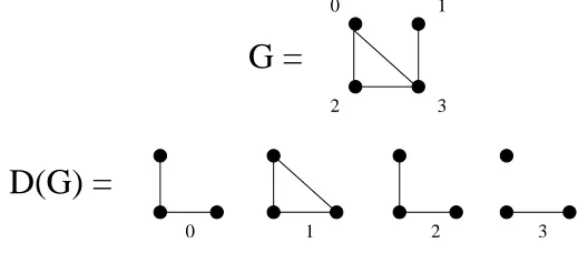
andE(F)∩E(G) =∅. If v is a vertex ofG, thenG−v is the graph obtained fromGby deleting vertexv and its incident edges – a vertex-deleted subgraph of G. The deck of G, D(G), is the multiset of vertex deleted subgraphs of G defined by [G−v0, ..., G−vn−1] where{v0, ..., vn−1} ∈V(G) and n=|V(G)|. Each member ofD(G) is referred to as a card. An example deck of a graph is given in Figure 1.

G =

0 1 2 3

D(G) =

0 1

2 3

Figure 1: Deck of graphG

In 1942, Kelly and Ulam proposed the Reconstruction Conjecture [4]. It states that every graph with three or more vertices is reconstructible up to isomorphism given its deck. In other words, given graphs G and H, D(G) = D(H)iff GandH are isomorphic. If true, then any graph with three or more vertices can be recreated simply by looking at its deck.

assume that any mention of the Reconstruction Conjecture in this report refers to reconstruction from vertex-deleted subgraphs.

It is known that the Reconstruction Conjecture does not hold for directed graphs. In 1977, Stockmeyer proved that there exists arbitrarily large directed graphs that are not reconstructible [4]. In the same year, Brendan McKay verified that the Reconstruction Conjecture holds for all simple, finite undirected graphs with nine or fewer vertices [4].

A more detailed survey of results regarding graph reconstruction can be found in [4, 5, 16]. Below is a detailed account of results regarding some classes of reconstructible graphs.

One important tool used to analyze the reconstructibility of graphs is Kelly’s Lemma. Given graphsF andG, let the number of subgraphs ofGisomorphic toF be denoted bys(F, G).

Kelly’s Lemma. For any two graphsF andGwhere|V(F)|<|V(G)|,s(F, G)

can be determined givenD(G)[9]. Proof.

s(F, G) = 1

|V(G)| − |V(F)|

X

v∈V(G)

s(F, G−v) (1)

The lemma results from the fact that the same occurrences of graphF in the subgraphs ofGwill be repeated|V(G)| − |V(F)|times inD(G). With this established, we can apply Kelly’s Lemma to reconstruct the number of edges in Gfrom its deck.

Corollary 1. Given D(G)of graph G,|E(G)|is reconstructible [9].

Proof. To find |E(G)|, we simply need to calculate s(K2, G). Obviously, the number of members in multiset D(G) is equivalent to |V(G)|. By applying Kelly’s Lemma, we can find |E(G)| simply by finding the total number of edges (equivalent to K2’s) in the subgraphs of D(G) and dividing this total by|V(G)| −2.

With further application of Kelly’s Lemma, it is possible to reconstruct the

degree sequence ofG. The degree sequence is the number of edges incident to each vertex ofG.

Corollary 2. Given D(G), the degree sequence ofG is reconstructible [9]. Proof. The number of incident edges of some vertex va, whereva ∈V(G) and

G−va is a card of D(G), is equivalent to s(K2, G)−s(K2, G−va). The

With these theorems established, it is possible to prove the reconstructibility of all regular graphs. When proving the reconstructibility of a class of graphs, it is customary to do so by proving that the class is bothrecognizableand weakly reconstructible [4].

Definitions 1. A class of graphs,C, is recognizable if, for each graph Gthat is a member ofC, every reconstruction of G is in C. A class of graphs, C, is

weakly reconstructibleif, for eachGthat is a member ofC, every reconstruction ofGthat belongs to Cis isomorphic toG[4].

Remark 1. Given the definitions, it follows that a class of graphs is recon-structibleiff it is both recognizable and weakly reconstructible.

Lemma 1. Regular graphs are recognizable [9].

Proof. The degree sequence of graphGis reconstructible givenD(G) by Corol-lary 2. The number of incident edges to each element ofV(G) are all equal iff

Gis a regular graph.

Lemma 2. Regular graphs are weakly reconstructible [9].

Proof. If we determine that graphG is a regular graph where each vertex has degreen, then by taking any card fromD(G), adding a vertex and connecting the new vertex to every vertex of the card with degreen−1 the original graph is reconstructed.

From this, we can conclude that all regular graphs are reconstructible [4]. The proof that disconnected graphs are reconstructible follows in a similar man-ner.

Lemma 3. Disconnected graphs are recognizable [9].

Proof. GraphG, where |V(G)| ≥3, is disconnectediff at most one card from D(G) is connected.

Lemma 4. Disconnected graphs are weakly reconstructible [9].

Proof. Take the largest order connected componentC from the cards ofD(G) where G is a disconnected graph. We know that this component must be a connected component ofG. A vertex,v, is known as acutvertex ofGiff there are more disconnected components inG−v thanG. Choose noncutvertexv0 wherev0∈V(C). Find the set of cards inD(G) with the least occurrences ofC as their components. From this set, choose the card with the most occurrences ofC−v0as its components. By taking this card and replacing one of theC−v0 components withC, the graphGis reconstructed.

1.2

k

-Reconstructibility

Kelly proposed that the Reconstruction Conjecture can be generalized by con-sidering the reconstructibility of graphs from subgraphs created by deleting some number k of vertices instead of just one [9]. The deck of graphG where each card is created by deleting a unique combinations of k vertices is denoted as Dk(G). Unless otherwise specified, references to the deck of G in this report

should be assumed to be regarding the singly vertex-deleted deck, orD1(G).

Definition 2. GraphGis said to be k-reconstructible iff it is uniquely recon-structible up to isomorphism givenDk(G).

As would be expected, given set S of all graphs of order n, ask becomes larger in comparison tonit is more likely that there exist someG∈Sthat is not k-reconstructible. In fact, for anyk >0, there must exist some graphsGwhere

|V(G)|= 2kthat are notk-reconstructible [4]. Determining the minimum value forf(k) such that all graphsGwhere|V(G)| ≥f(k) arek-reconstructible is still an open question that is much more difficult to resolve than the Reconstruction Conjecture.

1.3

Graph Reconstruction Numbers

An issue related to the Reconstruction Conjecture is that ofreconstruction num-bers. While the Reconstruction Conjecture is concerned with the possibility of reconstructing graphs from a deck, reconstruction numbers can be considered a measure of how easily a graph can be reconstructed from a deck. In most cases, a given graph G is reconstructible from a small subset of cards from

D(G). In fact, Bollob´as proved probabilistically that almost all graphs can be reconstructed with only three cards of a deck [3].

This project is concerned with two types of reconstruction numbers – the

existential reconstruction number and theuniversal reconstruction number.

Definitions 3. The existential reconstruction number of G, ∃rn(G), is the minimum number of vertex-deleted subgraphs ofGrequired to uniquely recon-structG up to isomorphism. Theuniversal reconstruction number, ∀rn(G), is the minimum number nfor which all multisubsets of D(G) of sizen uniquely reconstructGup to isomorphism.

Where a value for ∃rn(G) is found for graph G, we know thatG is recon-structible. In case there exists a graph G that is not reconstructible, we say that∃rn(G) =∞.

This report is only concerned with graphs with three or more vertices. The minimum existential reconstruction number for all of these graphs is three [2, 7].

G,vaandvb, we can produce a graphHthat shares the subdeck{G−va, G−vb}

by copying graphGand inverting the edge between va andvb.

Much has been proven regarding the existential reconstruction numbers of disconnected graphs thanks to work done by Wendy Myrvold and others [14, 15].

Theorem 1. Given disconnected graph G where not all components are iso-morphic, ∃rn(G) = 3 [15].

This was done by providing algorithms for choosing three vertices for discon-nected graphs where not all components have the same order and discondiscon-nected graphs with all components of the same order but not all isomorphic, and argu-ing that the deletion of these vertices result in subdecks unique to the original graphs. Problems with this proof were identified and corrected by Molina [14], but the results remain correct.

Theorem 2. Given disconnected graphGcomposed of isomorphic components, each component of order c,∃rn(G)≤c+ 2[15].

With the use of the above theorem, Myrvold found a method for calculat-ing∃rnfor any disconnected graph composed entirely of isomorphic, complete components.

Theorem 3. Given disconnected graph G of the form pKc, ∃rn(G) = c+ 2

[15].

Proof. Given disconnected graph G of the formpKc, D(G) consists of|V(G)|

elements of subgraph (p−1)Kc∪Kc−1. Consider disconnected graphH of the form Kc+1∪(p−2)Kc∪Kc−1. By deleting each vertex of Kc+1 from H we recreate the only multisubdeck of G of size c+ 1, meaning ∃rn(G) > c+ 1. Since applying Theorem 2 reveals that∃rn(G) ≤c+ 2, we can conclude that

∃rn(G) =c+ 2.

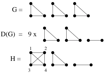
Using graph 3K3 as an example, the above proof is illustrated in Figure 2. Removing each numbered vertex from graphH, we recreatec+ 1 cards from D(G), pushing ∃rn(G) to five. As recently as 2002, Asciak and Lauri proved that this is the only class of disconnected graphs with such a high∃rnvalue.

Theorem 4. Given disconnected graph G of the form pC where C is not a complete subgraph, ∃rn(G)≤c [1].

2

General Project Description

Jennifer Baldwin first composed a project on calculating and analyzing exis-tential and universal reconstruction numbers for graphs. The calculations were performed for all graphs G where 3 ≤ |V(G)| ≤ 8 and some graphs where

2

G =

D(G) = 9 x

H =

1

3 4

Figure 2: Disconnected graph composed of 3K3components with ∃rn(G) = 5

up to order ten and for a class of graphs of order eleven – raising the number of graphs analyzed to approximately 12,294,000. Also, in this project I focus on the reasons certain graphs have unusually high reconstruction numbers and attempt to organize these graphs into classes to identify graphs of all orders with high reconstruction numbers.

Although no source code was used from Baldwin’s original implementation, the same basic algorithm was used with many enhancements for the sake of efficiency. Both the algorithm and the enhancements are outlined here. In the proposal, it was hoped that reconstruction numbers for all graphs with up to eleven vertices would be calculated. This report argues this is not currently feasible given constraints of time and processing power.

Lastly, calculations were performed to find non-trivial examples of graphs that are not 2-reconstructible. This was done in response to an email sent by Geoff Exoo of Indiana State University to Stanis law Radziszowski of the Rochester Institute of Technology on October of 2004. It states in part:

Specifically, I’d like to know: What are the largest known graphs that are not (set) k-reconstructible, for k > 1. One can search through all small graphs and find examples: there are graphs of order 11 that are not set 4-reconstructible, graphs of order 9 that are not set 3-reconstructible, etc. But non-trivial examples fork= 2 appear to be rare.

3

Graph Reconstruction Calculations

3.1

Algorithm Overview

The algorithm for calculating Graph Reconstruction Numbers involves compar-ing the decks of graph G to the decks of a select set of graphs to determine minimal reconstruction numbers forG. Here the set of graphs considered is the set of allsingle vertex extensions of the cards ofD(G). Pseudocode for finding

∃rn(G) of input graph Gis given in Algorithm 1. Details regarding extension graphs and evaluating all possible subdecks of a given size are below.

Algorithm 1General algorithm for computing∃rn(G) 1: Input graphG

2: AcquireD(G)

3: Acquire all 1-vertex extensions of each card ofD(G)

4: Acquire the deck of each extension graph

5: forsubdeck size= 2 ton−1 do

6: foreach subdeck ofGof sizesubdeck sizedo

7: _{f ound= false}

8: foreach extension graphdo

9: if extension deck contains current subdeck ofGthen

10: f ound= true

11: break out of innermost for loop

12: end if

13: end for

14: if f ound= falsethen

15: break out of outermost for loop

16: end if

17: end for

18: end for

19: The value ofsubdeck sizeis∃rn(G)

Then vertex extensionsof a given graphGis the set of all graphsH where there exists a subset ofnvertices fromV(H) such that H−v1−...−vn ∼=G.

So the order of everyn vertex extension of G is |V(G)|+n. Given graph G, the set of allsingle vertex extensions to each card fromD(G) is, by definition, the set of all graphs sharing at least one card in their decks with that ofD(G). The maximum number of possible single vertex extensions of given graphF is 2|V(F)|_{, but the actual number is usually much less given isomorphism.}

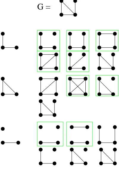
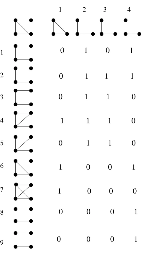
G =

After finding the unique extension graphs for each card of D(G), matches between the cards ofD(G) and the cards of extension graphs’ decks are repre-sented by arelation matrix. An example is given by Figure 4. The first row shows graphG and its deck, while following rows show extension graphs and unique matches marked between their cards and the cards ofD(G). It is impor-tant to put isomorphically equivalent cards fromD(G) adjacent to each other as shown in columns two and three of Figure 4. Also, matches to repeated cards of D(G) from an extension deck must be filled in from left to right, as illustrated in row one of Figure 4. Otherwise, it would be difficult to determine the set of all possible subdecks ofGof a given size.

With the relation matrix in place, the existential reconstruction number ofG can be found. We begin by assigning variablesubdeck sizea value of 2. Then every subset of D(G) of size subdeck size is examined to determine if there exists a multisubdeck ofGof sizesubdeck sizethat is not contained in any of the decks of the extension graphs. If so, then the current value ofsubdeck sizeis equivalent to∃rn(G). Otherwise,subdeck sizeis incremented and the process is repeated. As long asGis reconstructible, an existential reconstruction number will be found.

In the example diagram, we can see that no matter what two unique cards we choose from D(G), by reading down the columns in question we come up with at least one instance of two matching cards from an extension graph deck. Specifically, the unique subdecks evaluated in order are from columns {1,2},

{1,4}, {2,3} and {2,4} – each revealing at least one extension graph with a matching subdeck. Therefore, ∃rn(G) >2. Incrementing the subdeck size to three, we first evaluate the subdeck from columns{1,2,3}and find a match at row four. However, we next find a unique subdeck ofGwhen we come to columns

{1,2,4}. ∃rn(G) = 3. If there had been a matching subdeck to {1,2,4}, we would have next examined rows{2,3,4} before evaluating the full deck ofG. Given these examples, the general algorithm for evaluating an exhaustive list of subdecks of a given size should be obvious.

Because the old and new algorithms for finding universal reconstruction num-bers were fundamentally different, these are discussed in detail separately in Sections 3.3 and 3.5.

3.2

Software Tools

There were two tools used to assist in the calculation of reconstruction numbers. One of these, the Condor package [6], which is installed on several machines in labs at RIT, distributes the computation workload among several machines according to which machines have the most available processing time. This provided parallel processing that was essential for completing calculations in reasonable time.

3

0 1 1 0

1 1 1 0

0 1 1 0

1 0 0 1

1 0 0 0

0 0 0 1

0 0 0 1

0 1 1 1

0 1 0 1

1 2 3 4

1

2

4

5

6

7

8

9

manipulation functions. This is currently the most efficient software package available for identifying isomorphisms between graphs.

Graphs manipulated in thenautypackage were commonly presented in what is known asgraph6implementation. This is a string of ASCII characters used to denote the graph’s order with the first character and a packed adjacency matrix with all characters following. As an example, the graph referred to asG in Figure 1 is CN ingraph6notation. Each validgraph6representation of a graph has a single canonized labeling, also represented ingraph6. Two graphs have the same canonical labelingiff they are isomorphs.

3.3

Old Implementation Details

Jennifer Baldwin’s method for calculating reconstruction numbers depends heav-ily on files to avoid repeating calculations and save on processing time. In her implementation, the first step in finding reconstruction numbers for a set of graphs is to calculate all single vertex extended graphs and single vertex deleted graphs that will be needed. The results for these calculations are stored in two different files – one for extensions and the other for deletions.

Given an input file of graphs ingraph6format, programsshrink andexpand

produce canonized graphs in graph6 format for single vertex deletions and extensions, respectively. The output for the two programs are saved to two different files. The programreconstruct uses these two files to find extension files and decks needed by input graphs to calculate their reconstruction numbers.

Reconstruct cannot find the reconstruction number of an input graphGunless D(G) and the extension graphs of the cards ofD(G) are present in these files.

For each input graphG,reconstruct first scans the givenshrink file from the beginning, looking for the entry forD(G). Once found, the program takes the unique cards ofD(G) and searches for the set of extension graphs of each one from the beginning of the expand file. Once the set of appropriate extension graphs are identified, each one of their decks is found by scanning theshrink file from the beginning. Finally, an entry is made in the relation matrix for each extension graph so that the cards of its deck are related toD(G).

With the relation matrix formed, the existential reconstruction number of Gis computed as specified in Section 3.1. Looking at Algorithm 1, Jennifer’s algorithm for acquiringD(G), extensions of cards from D(G) and their decks entails scans of the pre-generated files.

It is obvious that the universal reconstruction number cannot be smaller than the existential reconstruction number. As a result, the calculated∃rn(G) value is used as the first value to test as being ∀rn(G). After ∃rn(G) is as-signed to variable curr sz, the program checks whether all subdecks of D(G) of sizecurr szare unique to D(G) by looking down the proper columns of the relation matrix. If an extension deck is found with the same subdeck being examined thencurr szis incremented, and the process is repeated. Otherwise,

∀rn(G) =curr sz. A universal reconstruction number will be found as long as

Algorithm 2Old algorithm for computing∀rn(G)

1: forsubdeck size=∃rn(G) ton−1do

2: f ound= false

3: foreach unique subdeck ofGof sizesubdeck sizedo

4: foreach extension graph from∃rn(G) algorithmdo

5: if extension deck contains current subdeck ofGthen

6: f ound= true

7: break for on line 3

8: end if

9: end for

10: end for

11: if f ound= false then

12: break for

13: end if

14: end for

15: The value ofsubdeck sizeis∀rn(G)

3.4

Comments on Old Implementation

Using the old implementation, Jennifer was able to complete reconstruction number calculations for all graphs with eight or less vertices. However, when the program was applied to graphs with nine vertices, the calculations for a single graph would take anywhere from one second to a full minute to complete [2]. Given that there are 274,688 graphs with nine vertices, completing the calculations would be too time-consuming even considering the gains achieved by Condor.

In Jennifer’s project, it was mentioned that file I/O was the major bottle-neck. Looking at the implementation, it is easy to see why. The calculations required for the reconstruction numbers of a single graphG entails sequential scans through text files forD(G), the extensions of the cards ofD(G) and the decks for each extension. As the order of graphs we want to analyze increases, the number of possible graphs we need to consider increases rapidly. This leads to much larger files and, consequently, much longer seek times to find the data we need. To split up the sets of graphs we want to consider to reduce the size of extension and shrink files is difficult to manage. Indeed, as the order of graphs grows the amount of time spent on file I/O is much more of a performance hit than what we are trying to save from processing time.

3.5

Current Implementation Overview

Whereas the old implementation depended on extension graphs and vertex deleted subgraphs being calculated beforehand and placed into files, the current implementation simply calculated these graphs as they were needed. Although the calculations of extensions and decks of the same graphs are repeated in this scenario, the more severe time-loss to CPU waits on file I/O were eliminated.

Although it is conceivable that the extension graphs and deck of each graph can be stored in memory when first needed and retrieved again for the recon-struction number calculations of each subsequent graph that needs it, this is sim-ply not feasible without very sophisticated methods. There are over 12,000,000 graphs with ten vertices and over 1,000,000,000 graphs with eleven vertices. This is especially sobering when we consider that there can be up to 2|V(G)| possible single vertex extensions of graphG. Also, the calculations of the deck of a graph take up so little processing time that they are hardly worth the ef-fort. Lastly, since the reconstruction number calculations will be done by many programs running on Condor, it makes sense to keep their memory footprints reasonably small since they will need to be migrated as other users log onto the machines in the lab.

Another big issue to consider in the old implementation is the algorithm for finding universal reconstruction numbers. Although it is guaranteed to obtain the correct result, the old method performs far more work than is needed. The only information needed to find ∀rn(G) is the maximum number of matches between the cards ofD(G) and the extension graphs’ decks. This information can be easily obtained as the relation matrix is set up. Adding one to this max-imal value yields the universal reconstruction number since this is the smallest subdeck size,s, where all possible subdecks ofD(G) of sizesare unique when compared to the decks of relevant extension graphs.

We can also improve the efficiency of our calculations when we observe that universal and existential reconstruction number values are always the same be-tween two complementary graphs [7]. Knowing this we can calculate reconstruc-tion numbers for approximately half of all graphs of a specified order, and simply assign these values to their complements. This is a little more difficult than it seems since we need to generate input graphs of a specified ordernsuch that they and their complements form the set of all graphs of ordernand no gener-ated graph is the complement of another genergener-ated graph. It is also important to note that some graphs areself-complementary – that is graphs Gsuch that G∼=G. If we blindly assign the reconstruction numbers of a self-complementary graph to its complement, we would be counting the same graph twice. Infor-mation on how input graphs are generated and assignment to complementary graphs are done properly is explained in the Section 3.6.

track of the maximal number of matches between extension decks and D(G). After the relation matrix is complete, incrementing this maximal value gives us

∀rn(G). If no extension graph entries end up in the matrix then∃rn(G) = 3. If there are extension graph entries in the relation matrix at this point, we begin looking at subgraphs of D(G) as specified earlier to find the smallest one possible that is unique among the extension decks. Whereas each row in Jennifer’s implementation is an array of values, the recent implementation simply uses a simple bitmap to represent the boolean match/non-match values. This makes calculation quicker as using a bitmask to represent the subgraph of D(G) we are looking at and performing a “bitwise and” with the extension deck in question quickly determines whether or not we have found a unique subdeck. Once we have found ∃rn(G) and ∀rn(G), these values are assigned to G if necessary. Situations in which we don’t assign these values to the complement are specified in Section 3.6.

Finally it must be noted that in the proposal for this project it was stated that we would use information we already know about reconstruction numbers for certain classes of disconnected graphs to save calculations. However, this was decided against since identifying disconnected graphs, their components and isomorphic equivalence between components may entail more calculations than they save. Also, letting the algorithm work on graphs with known reconstruction numbers helps test that it is functioning correctly.

3.6

Current Implementation Details

The generation of input graphs was performed using the geng program from Brendan McKay’snauty package. It is able to efficiently generate an exhaustive list of graphs of a specified class. Two properties of graphs thatgengcan specify are the number of vertices and minimum and maximum number of edges. The maximum number of edges possible for graph Gis n(n₂−1) where n =|V(G)|. Knowing this, we can generate all proper input graphs of ordernby tellinggeng

to create all graphs of ordernwith a maximum ofbn(n₄−1)cedges. Then we can safely calculate reconstruction numbers for each input graph and assign them to each corresponding complement. We need to be careful when we are doing cal-culations for graphs with an even number of maximum edges, however, as there exists graphs that have the same number of edges as their complements. So to avoid counting reconstruction numbers for the same graph more than once, the reconstruction numbers calculated for all graphs of ordernwith exactly n(n₄−1) edges are not assigned to their complements. The reconstruction numbers of these graphs and their complements must be computed separately.

gen-Algorithm 3Current algorithm for computing∃rn(G) and∀rn(G) 1: Program parameterorder specifies order of input graphs

2: totaledges= order(order−1)

2 ,maxedges=b

totaledges

2 c 3: Clearhash table

4: Clear listrel extensions

5: max matches= 2

6: Input graphGwhere |E(G)| ≤maxedges 7: ComputeD(G)

8: Compute all 1-vertex extensions of each card ofD(G)

9: foreach extension graphH computeddo

10: if H is not already inhash tablethen

11: AddH to hash table

12: ComputeD(H)

13: Setmatchesto the number of cards fromD(H) matching cards ofD(G)

14: if matches≥3then

15: AddH to rel extensions

16: max matches=max(matches, max matches)

17: end if 18: end if 19: end for

20: forsubdeck size= 3 ton−1 do

21: foreach subdeck ofGof sizesubdeck sizedo

22: f ound= false

23: foreach extension graphI inrel extensionsdo

24: if D(I) contains current subdeck ofGthen

25: f ound= true

26: break out of innermost for loop

27: end if

28: end for

29: if f ound= falsethen

30: break out of outermost for loop

31: end if

32: end for

33: end for

34: Thesubdeck sizeis∃rn(G) andmax matches+ 1 is∀rn(G)

35: if not(2|totaledges) or|E(G)| 6=maxedgesthen

36: Reconstruction numbers are assigned toG

necessary to write it to the relation matrix. This is not only important to save on memory used for the relation matrix but on processing time that would have been spent creating and canonizing the deck of an extension graph already avail-able for the input graph. Details in pseudocode of the new algorithm for finding

∃rn(G) and∀rn(G) for graphs of specified order are given in Algorithm 3. The last important implementation detail regarding reconstruction number calculations has to do with Condor. The calculation of reconstruction num-bers for all graphs with seven or less vertices is quick enough that the parallel processing power of Condor is not necessary. For these cases, the single recon-structionexecutable is run with the number of vertices specified as a command line parameter. This quickly generates output files containing reconstruction number counts and graphs with notably high reconstruction numbers.

For sets of graphs with more vertices, Condor is helpful. To use Condor, the calculation of reconstruction numbers were split up into three separate modules: one to generate input graphs, another to calculate reconstruction numbers for a set of graphs and a module to process reconstruction number output for sets of graphs as they are created. The proper invocation of these programs is coordinated by the run recon shell script. Parameters within the shell script can be changed to affect the maximum number of input files that can be present at the same time and the number of graphs within each input file, among other settings. Communication between these programs, which were scattered across several machines, is achieved with files stored on an NFS.

A specialized module was created to generate input since storing all input graphs into files at the same time would take up too much disk space. Instead, program createInput creates input files as they are needed by reconstruction number calculators assigned as Condor jobs. The createInput program creates a specified number of input files (as dictated byrun recon) forreconstructNums

jobs to work on in parallel. When a reconstructNums job is finished with its input file, it deletes it. WhencreateInput sees it needs to generate more input files it simply creates new ones containing input graphs from the point it left off. By specifying how many input filescreateInputmust keep present at a time, we are specifying how many Condor jobs are calculating in parallel.

A reconstructNums Condor job is submitted by run recon whenever a new input file is generated. Each of these jobs calculates reconstruction numbers for graphs in its assigned input file, deletes the input file, then generates one reconstruction number output file for existential data and another for universal data. It is these jobs that are utilized for parallel processing.

found to have a ∃rn value of four. Lastly come the ∃rn count totals – 569 graphs G where ∃rn(G) = 3 and and two graphs with a ∃rn value of four. The reason why results for more than 300 graphs were generated was that results for input graphs were also assigned to their complements when possible. Remember, assignment to complements is not done for input graphsGin cases where|E(G)|= |V(G)|×(|₄V(G)|−1). This explains why in the example the number of graphs assigned∃rnvalues is less than 600.

The filegraphs8u600.outis a summary of ∀rn calculations for the same set of graphs. First the exceptions given are the set graphs within the input set found with the highest∀rnvalues – in this case, six. These results are only kept for the final output of all graphs of order eight if no graphs of that order are found with higher∀rnvalues. If higher values are found,processOutput throws out these results in favor of the graphs with the highest ∀rn values. Finally come the∀rncount totals.

The last module,processOutput simply sequentially processes the existential and universal reconstruction number output files generated by all reconstruct-Nums, deleting them as it finishes each. When it has completed processing all of these files, it simply outputs two final output files, summarizing relevant reconstruction number data for existential and universal values.

The final output files generated byprocessOutput for graphs with eight ver-tices is given in Appendix A.2. As expected, graphs8e.out is a summary of

∃rnvalues for all graphs of order eight andgraphs8u.outis a summary of their

∀rn values. The existential reconstruction number summary shows all graphs G of order eight where ∃rn(G) > 3 and the ∃rn count totals for all graphs of order eight. Filesgraphs8u.out shows the set of all graphs of order eight with the highest∀rn(G) value and a∀rncount summary of all graphs of order eight. Notice that it threw out the exception results ofgraphs8u600.outsince graphs were found with a∀rnvalue of seven.

3.7

2-Reconstructible Calculations

The algorithm for determining whether or not a graph is 2-reconstructible is very similar to that used to calculate the reconstruction number of a graph. First, given graph G, D2(G) is found and each of the n₂ deck’s cards is canonized. Next, for every card ofD2(G), all possible 2-vertex extensions are found and canonized.

From card F of order n, there are 22n+1 _{possible extension graphs where} isomorphism is not taken into consideration. Similar to the new algorithm for finding reconstruction numbers, a hash table is used so that the same extension graph is not used twice when determining whether or not a single input graph is 2-reconstructible.

3.8

Run-time Complexity Estimates

When calculating reconstruction numbers for graphs, the majority of time was spent canonizing graphs. Thegprof profiling tool was used to analyze the recon-struction program when calculating the reconstruction numbers for all graphs with eight vertices. While running, the program spent 72.9% of the time in themakecanon() function – a function copied directly from thenautypackage which canonizes a given graph. The function was called a total of 34,519,304 times to calculate reconstruction numbers for the 12,346 graphs with eight ver-tices. Given a single input graphGof ordern, there are three major categories of graphs that must be canonized.

The first of these are all of the cards in D(G), requiring the canonization ofngraphs, each of ordern−1. These are used to set up the relation matrix, so that the decks of relevant extension graphs are related toD(G) according to isomorphic equivalence. This is only a very small fraction of the number of graphs needed to be canonized and does not take up a significant amount of processing time.

The second category of graphs needing canonization are all possible exten-sion graphs of unique cards from D(G). The number of these graphs varies from 2n−1 _{to 2}n−1_{×n depending on the number of unique cards in D(G).} Of course, all of these graphs are of order n. These calculation are used to establish the set of unique relevant extension graphs necessary for calculating reconstruction numbers forG. Ruling out repeated extension graphs saves us many canonizations in the next category.

The last category involves taking the extension graphs generated above and canonizing each card from their decks. The maximum number of graphs possible here is 2n−1_×n2_{. However, the actual total is likely to be much less when} isomorphism is taken into account.

For 2-reconstructibility of input graphG, we must canonize the n(n₂−1)cards of order n−2 that are in its deck. From these, a possible range of 22n−3 _to 22n−3_× n(n−1)

2 extension graphs of order n are canonized. Consequently, a maximum of 22n−3_×n(n−1)

2 ×

n(n−1)

Table 1: Number of graphs of specified order

Order Graph Set Size

1 1

2 2

3 4

4 11

5 34

6 156

7 1,044

8 12,346

9 274,688

10 12,005,168

11 1,018,997,864

Table 2: Running times with 55 machines working in parallel

Order of Graphs Time Finding Rec. Numbers Time Testing 2-Recon

8 2 min. 11 min.

9 24 min. 976 min.

10 1,969 min. n/a

11 787,600 – 1,440,000 min.a

n/a

for higher order input sets with 55 machines working in parallel. In practice, from finding reconstruction numbers for the first five million graphs with eleven vertices, calculations were completed for approximately one million input graphs every day. These considerations were used to come up with the estimated time for finding reconstruction numbers for all graphs with eleven vertices.

4

Results

4.1

Verifying Calculations

The reconstruction number calculations were verified by comparing them to calculations for smaller graphs performed by hand. In addition, the∃rnvalues calculated for disconnected graphs were compared to their expected values as predicted by Theorems 1, 3 and 4. All of these graphs were calculated to be in the range of their predicted values. Finally, the results had to be tested against results from Jennifer Baldwin’s project. Even though the two sets of results were extremely close, there were some discrepancies between them.

Where the counts of universal reconstruction numbers disagreed, it was proven that there was at least one graph of order eight with a high∀rnmissing from the Jennifer’s data set. In some cases, there were graphs found to have high existential reconstruction numbers in the recent calculations that were missing from the older data. In these instances, it was proven that newly generated graphs had at least the recently calculated reconstruction numbers.

Lastly, there were graphs from the older data set which were found with large existential reconstruction numbers that did not show up in the newer set. Unfortunately, it is much more difficult to disprove that a certain graph has a high reconstruction number. But given that discrepancies were extremely rare, and that in most of these cases they were proven to be in favor of the newer data, it is reasonable to assume that the current calculations are correct. More details on these findings are given in Section 4.4.

Since the algorithm for testing 2-reconstructibility was so similar to that used to find reconstruction numbers, we can safely assume that it is also correct. Just to be sure, graphs found not to be 2-reconstructible were easily verified by hand as the program output the two or more graphs with the same two vertex deleted decks.

4.2

High Existential Reconstruction Numbers

4.2.1 Disconnected Graphs Composed of Complete Components

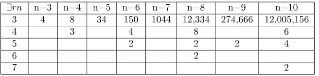
Table 3 shows the count of graphs with high existential reconstruction numbers arranged by order. When Jennifer analyzed her results, she hypothesized that there did not exist a graphGwith an odd number of vertices where∃rn(G)>3 [2]. However, we can see that there are two graphs with nine vertices with high reconstruction numbers.

Table 3: ∃rn(G) counts

∃rn n=3 n=4 n=5 n=6 n=7 n=8 n=9 n=10

3 4 8 34 150 1044 12,334 274,666 12,005,156

4 3 4 8 6

5 2 2 2 4

6 2

7 2

This is not surprising considering that Myrvold proved that for any discon-nected graphGof the formpKc,∃rn(G) =c+ 2 [15]. This being the case, we

can create graph 3K3 – a disconnected graph with nine vertices and an exis-tential reconstruction number of five. An example of this was given in Figure 2. This graph and its complement are the two graphs with nine vertices with a high reconstruction number.

Graphs 2K2, 2K4, 4K2, 2K3, 3K2, 3K3, 2K5, 5K2 and their complements were all identified as having the correct existential reconstruction number in the results. All of these graphs are explained in this category.

As an aside, it is easy to establish that for any composite number n there exists a graph G of ordern such that∃rn(G) > 3. This follows as a simple corollary of Theorem 3.

Corollary 3. Given non-prime integern, there exists a graphGwhere|V(G)|=n

such that∃rn(G)>3.

Proof. Given non-prime integer n and integer d ≥ 2 such that d|n, we can construct graphGof the formpKd. Applying Theorem 3,∃rn(G) =d+ 2.

However, this still does not answer whether or not there exists a graph G where |V(G)| is prime and∃rn(G) >3. In the results, no such example was found. It is unfortunate that reconstruction number calculations could not be completed for all graphs with eleven vertices since this would provide data for a much larger set of graphs with a prime number of vertices. It is interest-ing to note that all categories of graphs identified as havinterest-ing high existential reconstruction numbers require a non-prime number of vertices.

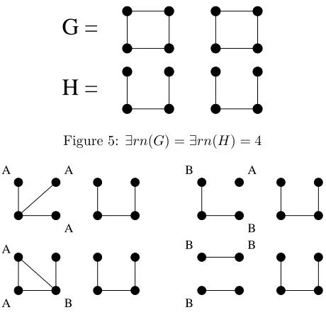
4.2.2 Other Graphs Composed of Isomorphic Components

H =

G =

Figure 5: ∃rn(G) =∃rn(H) = 4

B A

B A

B B

A A

A B B

A

Figure 6: Proof∃rn(H)>3

will recall that it was recently proved that ifGis a disconnected graph of isomor-phic components of orderc and the components are not isomorphs ofKc, then ∃rn(G)≤c[1]. There were only two graphs in this category found to have high existential reconstruction numbers, and both had the maximum value possible. They are shown in Figure 5.

Looking at Figure 5, with CG as a component of G, ∃rn(CG) = 4. The

reason for this is CG ∼= K2,2. Notice that every card in D(G) is the same. Therefore, there is one unique subset ofD(G) for any given subset size. When this holds true for disconnected graphs of isomorphic components, the existential reconstruction number must be at least as large as ∃rn(CG) – its component

graph.

As a side note, consider some general disconnected graphGof the formpC whereD(C) is composed entirely of isomorphic subgraphs. Since in this situa-tionD(G) is also composed entirely of isomorphic subgraphs then∃rn(G)≥ ∃rn(C). (See Proposition 2 for details). Combined with the knowledge that∃rn(pC)≤ |V(C)|

where C is not complete [1] it is proven that ∃rn(C) ≤ |V(C)| thus proving graphs, excluding the complete variety, whose deck are composed entirely of several instances of the same card are reconstructible.

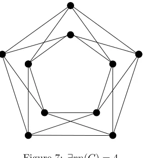
Figure 7: ∃rn(G) = 4

Proposition 2. For any disconnected graphG of the form pC where the ele-ments ofD(C) are all isomorphic, ∃rn(G)≥ ∃rn(C).

Proof. Given graphG of the formpC where the elements ofD(C) are all iso-morphic, it must also be true that the elements of D(G) are all isomorphic. There is only one unique subset ofD(G) for any given subset size. Given graph Hsuch thatD(H) has∃rn(C)−1 cards in common withD(C), we can compose disconnected graphI∼=H∪(p−1)C. GraphGshares ∃rn(C)−1 cards with I, forcing∃rn(G)≥ ∃rn(C).

With graphH from Figure 5, it is also the case that for its components,CH, ∃rn(H) =∃rn(CH). But unlike graphG, this fact cannot be easily established

without analyzing the cards ofD(H) and finding other graphs which contain every possible 3-card subdeck ofD(H) in their own decks.

Deleting each vertex from the top row ofH in Figure 5 creates a set of four isomorphic cards which we labelA, and deleting vertices from the bottom row ofH leaves us with another set of isomorphs to be labeledB. Figure 6 shows four graphs whose decks contain all possible multisubsets with three elements fromD(H). The labeled vertices indicate which can be deleted to recreate cards

AorB fromD(H).

When considering some disconnected graphGof the form 2CwhereCis not complete, we might wonder whether it must be true that∃rn(G)≥ ∃rn(CG).

No exception to this rule was found in the results. By using Theorem 4 and con-sidering that we already know that all complete graphs are reconstructible, we may deduce that to prove this would be to prove the Reconstruction Conjecture as well.

4.2.3 Regular Graphs of Redundantly Connected Cycles

9

D(G) = 10 x H =

0

1

2 3

4 ₅

6

7 8

Figure 8: H−v0'H−v4'H−v9'card ofD(G)

was identified in the results, but we can deduce that there are an infinite number of graphs that share this property.

GraphGis a regular graph where all cards in D(G) are isomorphic. Since all cards are isomorphic, there is one unique subset ofD(G) for any given subset size. So to prove that∃rn(G)>3, we only need to construct one graph that shares three cards in its deck with that ofD(G). This is shown in Figure 8.

The graph on the left is isomorphic to every card in D(G). The graph on the right,H, is a graph that is not isomorphic toGthat contains three copies of the cards from D(G) in its own deck. These cards are created by deleting verticesv0,v4 andv9.

The reason this works is simple. Notice how vertices v4 and v9 are both connected to v3, v5 and v8 and no others. We composeH by adding v0 and connecting them to these vertices shared byv4 andv9. With this established, if we delete eitherv4orv9then by movingv0to the place of the deleted vertex while preserving its edges, we have reproduced the graph on the left – the two are isomorphic. And of course, deleting v0 will recreate the card as well. It is also true that connections to same vertices occurs between v6 and v1, v2 and v7, andv3 andv8. In short, it holds for any two vertices from the card ofD(G) that appear in the inner and outer polygon and are spatially adjacent to each other. Composing a new graph using any of these two sets of vertices to dictate the connections of v0 will also create a graph with three cards in its deck in common withD(G).

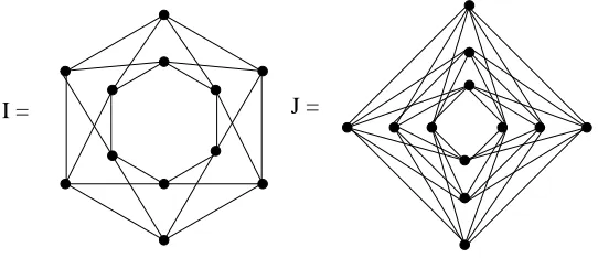
I = J =

Figure 9: ∃rn(I)>3 and∃rn(J)>4

graphs of redundantly connected cycles.

First, a few new symbolic conventions are needed. C(G) is the set of cycles of graph G. Notation va ∼ vb states that vertex a is connected to vertex b.

Finally, for the following definitionvc,i identifies vertexiof cyclec.

We define RCC(n, l) to be a regular graph with nredundantly connected cycles, each of lengthl. So in Figure 9I∼=RCC(2,6) andJ ∼=RCC(3,4). To compose a graph Gof the form RCC(n, l) we begin with graphF where F is the union of n cycles, each of length l. Let the vertices of each c ∈ C(F) be labeled such thatvc,i∼vc,(i+1)mod lwhere 0≤i≤l−1. Then by adding edges

between the cycles of F such that vc,i ∼ vd,(i+1)mod l where c 6=d we create

graphGof the formRCC(n, l).

Theorem 5. Given graph G, of the form RCC(n, l),∃rn(G)> n+ 1.

Although graphs in this category appear among the set of graphs with six, eight and nine vertices, their high∃rnvalues were accounted for by other reasons as RCC(2,3)∼=K2,2,2, RCC(3,3)=∼K3,3,3 and RCC(2,4) ∼=K4,4. Since the complement of any disconnected graph of the formpKc is a connected graph

whose deck contains isomorphic elements, it is not surprising that there is some overlap between them and the graphs in this section. The following remarks show two classes of graphs that have this overlap as a property.

Remark 2. Given graphGof the formKc,cwhere 2|c,G∼=RCC(c₂,4).

Remark 3. Given graphGof the formKc,c,c,G∼=RCC(c,3).

Given Remark 2, we can see that graphJ from Figure 9 is an isomorph of K6,6. It may be the case that there are other classes of graphs that also belong to these two categories simultaneously.

Finally, since graphs in this category have decks containing all isomorphic elements, given Proposition 2 we can build other disconnected graphs with large

∃rnvalues. The result is the following corollary.

Figure 10: Examples of 1-1 connectedKc pairs

Table 4: ∃rn values for connectedKc pairs

G ∃rn(G)

K3↔2K3 4

K4↔2K4 4

K4↔3K4 5

K5↔2K5 4

K5↔3K5 5

K5↔4K5 5

4.2.4 Pairs of Complete Graphs Connected by 1-1 Edges

For some graphGto be in this categoryGmust be made entirely of two complete Kc subgraphs which are connected to each other by b edges where 2≤b < c.

Finally, each vertex must be connected to at most one vertex from the opposite Kc. Examples are given in Figure 10.

Because the two subgraphs being connected are complete, a description of the order of the complete subgraphs and the number of one-to-one edges connecting them specifies a single, isomorphically unique graph. Looking at Figure 10, the given graphs can be labeled as K3 ↔2 K3, K4 ↔2 K4, K4 ↔3 K4 and K5↔3K5.

To understand why the graphs in this category have large∃rn values, we must consider the contents of their decks. Every graph of this type has exactly two sets of cards in its deck.

Theorem 6. For any graph G of the form Kc ↔b Kc where 2 ≤ b ≤ c−1, ∃rn(G)>3.

Unpredicted Graph Sharing

Predicted Graph Sharing

3 Cards with D(G)

G =

Original Graph

3 Cards with D(G)

Figure 11: Graph exception with high∃rn(G)

copies ofB.

Given graphKc+1↔b−1Kc−1, which we label graphH, a subgraph isomor-phic to A is created for each vertex deleted from Kc+1 not connected to the labeledKc−1. This means thatH containsc−b+ 2 copies of A in its deck. But since we assumed thatc > bin graphG, the deck ofH contains at least three copies of A.

With graphKc+1↔bKc−1, which we label graphI, a subgraph isomorphic toAis created with each vertex deleted fromKc+1that is not connected to the oppositeKc−1, and we attain a subgraph isomorphic to B for each remaining vertex we delete from theKc+1piece. This gives usbcopies ofAandc−b+ 1 copies ofBinD(I). Since we assume thatb≥2 for graphG, that leaves us with at least two copies ofAinD(I) and asc > bthere are at least two isomorphs of B inD(I). Therefore, fromD(I) we can extract a multisubset with two copies ofA and one copy ofB and a multisubset with two copies ofB and one copy ofA.

Finally we considerKc+1 ↔b+1 Kc−1, or graphJ. By deleting each vertex from the Kc+1 piece that is connected to Kc−1 by one of the b+ 1 edges, we obtain an isomorph ofB. Asb+ 1≥3 this leaves us with at least three elements isomorphic toB fromD(J).

With these graphs and their noted subdecks we know∃rn(G)>3.

In some cases, we can prove that the existential reconstruction number must be higher for graphs in this class. An example is illustrated by the following proposition.

Proposition 3. Given graph Gof the formKc↔c−1Kc,∃rn(G)≥c.

Table 5: Predicted graphsGwhere∃rn(G)>3 and|V(G)|= 12

Minimum∃rn Predicted GraphsGWhere|V(G)|= 12

4 6K2/6K2

3K2,2/3K2,2

RCC(2,6)/RCC(2,6)

{K6↔bK6 |2≤b≤4}/{K6↔bK6|2≤b≤4}

5 4K3/K3,3,3,3

6 3K4/K4,4,4

K6↔5K6/K6↔5K6

8 2K6/K6,6

4.2.5 High∃rn Exception

The only graph identified with a high existential reconstruction number that did not fit neatly in the above categories wasK2 ↔1 K2 having ∃rn(G) = 4. Although it is technically a pair of complete graph connected by a one-to-one edge, there are too few one-to-one edges to use Theorem 6 and the complete graphs connected are too small to use Proposition 3 to prove a high existential reconstruction number.

There are two possible multisubsets of size three in its deck. One graph that contains one of these multisubsets in its own deck isK3↔1K1, which fits one of the graph constructions used in the proof of Theorem 6 (Kc+1 ↔b Kc−1). However, the graph sharing the other possible three card subdeck does not match any graph constructions used in proofs from the previous section. This is illustrated in Figure 11. But sinceK2↔1K2 has so few vertices, it may just be a degenerate case. It is also notable that this graph is its own complement, explaining the odd number of graphs of order four with∃rn(G) = 4.

4.2.6 Predicting Graphs with High ∃rn

Given what we know about categories of graphs with high existential reconstruc-tion numbers, we can predict a number of graphs with some given number of vertices where∃rn >3. Here we will use the set of graphsGwhere|V(G)|= 12 for an example.

The first graphs we can look for are disconnected graphs of the form pKc

simply by considering multiples of the order in question. For graphs of order twelve these graphs are 2K6, 3K4, 4K3and 6K2. The∃rnvalues for all of these graphs arec+ 2 for themselves and their associated complements.

Next we can consider graphs of the form Kc ↔b Kc where 2 ≤b ≤c−1.

H????CK

EAMW G?D@\g

Figure 12: Example graphs with maximal∀rn values

there is currently no known easy method for determining which of these graphs have high ∃rn values, there are a few specific graphs of this form to consider. First of all, we know that where graphG is K2,2, ∃rn(G) = 4. Given Propo-sition 2 and Theorem 4, we can deduce that for any graphH of the form pG,

∃rn(G) = 4. So among the set of graphs of order twelve, 3K2,2and its comple-ment has an∃rn value of four. Other graphs to check within the set of graphs of ordernwould be disconnected graphs of the formpC wherep|nandC is of the form RCC(n, l). However, in the case where n = 12, all possible regular graphs of this form are already accounted for as complements of disconnected graphs of the formpKc.

The last category of graphs is the set of possible of RCC graphs of the specified order. In the case of order twelve, these graphs composed of cycles of length three and four have already been accounted for given Remarks 2 and 3. This leaves only RCC(2,6) (graph I from Figure 9) and its complement. Consequently,∃rn(I)≥4 and ∃rn(I)≥4. These predictions are summarized in Table 5.

4.3

Universal Reconstruction Number Statistics

The universal reconstruction number totals arranged according to order are given in Table 6. Although it has been proven that for the majority of graphs Gthat∃rn(G) = 3, the calculated∀rnvalue totals seem to indicate there is no single universal reconstruction number that holds for the majority of graphs.

For this data set, the maximum count of ∀rn values among graphs of a specified order seems to change unpredictably. Surprisingly enough, this maxi-mum count for graphs of order ten was for∀rn(G) = 3. This only occurs again in the results among graphs of order three. For most graphs G in Table 6, 3 ≤ ∀rn(G) ≤ 5, but in the absence of additional information this may not remain true as the order of graphs considered increases.

8

G = H =

H????CK H????cK

1

6

4 5

0 2

4 5

6 7 8 0 1 2 3 3

7

Figure 13: ∀rn(G) =∀rn(H) = 7

Table 6: ∀rn totals

∀rn n = 3 n = 4 n = 5 n = 6 n = 7 n = 8 n = 9 n = 10

3 3 2 7 8 16 266 45,186 6,054,148

4 9 19 56 496 8,308 199,247 5,637,886

5 8 90 520 3,584 28,781 301,530

6 2 12 284 1,434 10,686

7 4 20 914

8 4

Figure 12 shows examples of graphs with maximal∀rnvalues among the set of graphs of order six, eight and nine. It is interesting to note that where graph Gis H????CK ingraph6 notation,∃rn(G) = 3 according to Theorem 1, and yet∀rn(G) was calculated to be as high as seven.

Figure 13 explains this property for graph H????CK. GraphG (H????CK) and graphH (H????cK) have six cards from their decks in common. Deleting verticesv0, v1, v2 and v3 from both graphs create four of these common cards and deleting vertices v4 and v5 from both create the other two, proving that

∀rn(G)≥7 and∀rn(H)≥7. By applying the algorithm from [14], the arrows in the figure point to three vertices fromG and H whose deletion will create unique subdecks for each. ∃rn(G) =∃rn(H) = 3.

4.4

Discrepancies Between Old and New Data Sets

4.4.1 ∃rn Discrepancies

The ∃rn(G) counts found in old and new data sets matched perfectly where 3≤ |V(G)| ≤8. The ∃rn(G) values for individual graphs also matched where 3≤ |V(G)| ≤7. However, the graphs of order eight found with high ∃rn and their values differed slightly between the two.

Figure 14: Unmatched graphs from old data set

Table 7: ∀rntotal discrepancies where|V(G)|= 8

∀rn(G) Old Totals Current Totals

4 8,209 8,308

5 3,576 3,584

6 292 284

7 3 4

∃rnvalue in the old data, indicating an error. Graph 2[K2↔1K2] was another graph proven to have a high∃rnthat was missing from the old calculations.

Another graph with a high∃rnvalue missing from the old data wasK4↔3K4. Because of Proposition 3, we know that ∃rn(G) ≥ 4. The ∃rn value for this graph in the new data was five. The graph’s complement was also missing from the old data.

Three graphs of order eight which were identified in the old data as having high∃rnvalues which were not found in the new data are given in Figure 14. It may be the case that these graphs were simply not drawn correctly in the old writeup. Unfortunately, the graph6labels of these graphs were not available from the old data to check whether this was the case.

4.4.2 ∀rn Discrepancies

The totals for ∀rnvalues for all graphs Gwhere 3 ≤ |V(G)| ≤7 found in the old and new results agreed. However, the totals for graphs with eight vertices were not the same. These differences are shown in Table 7.

G?CrUW

0 1

2

3

4 5

6 7

0 1

2

3

4 5

6 7

H =

G =

G?D@\g

Figure 15: Two graphs with∀rnvalues≥7

four graphsGwhere|V(G)|= 8 and∀rn(G)≥7. Although this does not prove the correctness of the new data, at least we know that it should not exactly match the old data set.

Figure 15 shows two graphs who share six cards between them from their decks. They are labeled according to theirgraph6notation fromnauty. The six matching cards areG−v0andH−v1,G−v1andH−v3,G−v2andH−v4, G−v3 and H −v5, G−v4 and H −v6, and finally G−v5 and H−v7. By confirming by hand, we can verify that each pair of subgraphs are isomorphs, and no pair is isomorphic to another. The six shared cards confirms that both

∀rn(G) and∀rn(H) must be at least seven.

Furthermore,G has eight edges whileH has ten. Given that a graph with eight vertices can have a maximum of 28 edges, it is not possible thatG and H are complements of each other nor can it be the case that eitherGorH are complements of themselves. So not only must ∀rn(G) ≥ 7 and ∀rn(H) ≥ 7, but∀rn(G)≥7 and∀rn(H)≥7 as well. There must be at least four graphsG where|V(G)|= 8 and∀rn(G)≥7.

4.5

Graphs That Are Not 2-Reconstructible

Calculations testing the 2-reconstructibility of graphs was completed for all graphsGwhere |V(G)| ≤9. In these calculations, seven of the eleven possible graphs with four vertices were found not to be 2-reconstructible. This is not surprising considering the low number of vertices compared to the number being deleted.

There were four graphs found with five vertices that were not 2-reconstructible. These were the two graphs pictured in Figure 16 and their complements. It is easy to verify by hand that these two graphs have the same 2-vertex deleted decks.

Figure 16: Two graphs with the same 2-vertex deleted decks

that all graphs, G, where |V(G)| ≥ n are reconstructible from Dk(G)? The

Reconstruction Conjecture assumes that when k = 1, the minimum order is three.

Some notable properties of the two graphs in Figure 16 are that one is a tree while the other is a disconnected graph. What is notable is that although both trees and disconnected graphs have been proven to be reconstructible when just one vertex is deleted, this does not hold for 2-reconstructibility.

5

Conclusions

The resulting data and analysis from this report point to several topics that are worth further research. Most interesting of these is the question of whether there exists any graphsGwith a prime number of vertices such that∃rn(G)>3. In addition, when considering the categories of graphs identified as having high existential reconstruction numbers, it is worth examining whether there are additional categories to be found containing higher ordered graphs. Also, can we find a more precise range of possible ∃rn values for categories of graphs identified in this report? Specifically, it seems that with a bit more analysis we may easily narrow the range of possible∃rn values for graphs of the form Kc ↔b Kc. Lastly we come to the topic of 2-reconstructibility. Of all graphs

analyzed for 2-reconstructibility, graphs Gwhere 3 ≤ |V(G)| ≤9, two graphs of order five and their complements were identified as the graphs with the most vertices to not be 2-reconstructible. Could it be the case that for all graphs G where |V(G)| > 5, G must be 2-reconstructible? These considerations are discussed in more detail below.

First and foremost, do there exist any graphs G of prime order such that

∃rn(G)>3? Since the explanations behind high∃rn values identified depend on a non-prime number of vertices, the data seems to suggest that they do not. However, this does not disprove their existence. Completing reconstruction number calculations for graphs with eleven may help, but they can only solve the question by identifying a graphGwith eleven vertices where∃rn(G)>3.

The next question to consider is whether or not there are graphs with high

the only categories of graphs with high∃rnvalues. It may even be the case that no finite set of categories can encompass all graphsGwith∃rn(G)>3.

Notice that in the discussion of categories of graphs identified with high∃rn values, much of the work was put into establishing lower bounds for existential reconstruction number values. It would be more interesting to establish upper bound ∃rn values instead. Due to prior research, the exact value of ∃rn(G) for disconnected graphs of the formpKc, and an upper bound∃rn(G) for

dis-connected graphs of the formpC are already known. However, little is known regarding upper bound∃rnvalues for graphs of the formKc↔bKcand regular

graphs of redundantly connected cycles. We know that for anyRCC graphG that ∃rn(G) ≤ |V(G)| since regular graphs are known to be reconstructible. But the reconstructibility of graphs of the form Kc ↔b Kc is still open, and

may be easy to establish.

While on the topic, given a graphGof the formKc↔bKc, can we useband

cto calculate the exact value for ∃rn(G)? This report only establishes that all graphs of this form must have high∃rnvalues and gives a tentative lower bound for graphs of the formKc↔c−1Kc. This leaves much room for improvement.

From the topic of 2-reconstructibility comes the question of whether there exists any graphs G where |V(G)| > 5 such that G is not 2-reconstructible. This probably will not be solved any time soon since the seemingly easier ques-tion of whether there exists any graphs G where |V(G)| ≥ 3 that are not 1-reconstructible (the Reconstruction Conjecture) is still an open question.

Finally, we must consider if there are ways to significantly improve the ef-ficiency of the algorithms employed to calculate reconstruction numbers. One portion to consider would be the generation of all possible extension graphs of a given graph. In the current implementation, 2|V(G)| _{extensions of graphGare} exhaustively generated and canonized although the resulting set of isomorphi-cally unique extension graphs usually turns out to be much smaller. However thegeng program from the nautypackage, which can generate an exhaustive set of isomorphically unique graphs of a given order, does no canonization to generate its results unless the user specifies that she wants the output presented in canonized form. If we can find a method to generate extensions of graphs that significantly cuts back on the number of calls to the expensivemakecanon()

A

Sample Output Files

A.1

Output Files from

reconstructNums

Listing of graphs8e600.out:

Exceptions 4 G‘?G?C

Complement G]~v~w Totals

3 569

4 2

Listing of graphs8u600.out:

Exceptions 6 6 G??tY{

Complement G~~Id? 6 G?B@x{

Complement G~{}E? 6 G??xuK

Complement G~~EHo 6 G?@XvO

Complement G~}eGk 6 G?@Xvo

Complement G~}eGK 6 G?Bapo

Complement G~{\MK 6 G?AZRo

Complement G~|ckK 6 G??~Uo

Complement G~~?hK 6 G?AZvo

Complement G~|cGK 6 G@Ge}w

Complement G}vX@C 6 G?B\ro

Complement G~{aKK 6 G?Azvo

Complement G~|CGK 6 G?@~vo

6 G?O__[

Complement G~n^^_ 6 GGC?KK

Complement Gvz~ro 6 G?O_c[

6 GGC?G{

Complement Gvz~v? Totals

3 6

A.2

Output Files from

processOutput

Listing of graphs8e.out:

---4 G‘?G?C

Complement G]~v~w ---4 G?‘H?c

Complement G~]u~W ---4 GoCOZ?

Complement GNznc{ ---5 GoSsZc

Complement GNjJcW ---4 G‘iayw

---6 G~?GW[

Complement G?~vf_ ---4 G‘rHpk

Existential Reconstruction # Totals 3 12334

4 8

5 2

6 2

Listing of graphs8u.out:

Exceptions 7

---7 G?D@\g

Complement G~y}aS ---7 G?CrUW

Complement G~zKhc

Universal Reconstruction # Totals 3 266

4 8208 5 3584 6 284

References

[1] K. J. Asciak and J. Lauri, On Disconnected Graph with Large Reconstruc-tion Number.Ars Combinatoria, 62:173-181, 2002.

[2] J. Baldwin, Graph Reconstruction Numbers, Master’s Project, Rochester Institute of Technology, 2004.

[3] B. Bollob´as. Almost every graph has reconstruction number three.Journal of Graph Theory, 14(1):1-4, 1990.

[4] J. A. Bondy. A Graph Reconstructor’s Manual.Surveys in Combinatorics, 1991 (Guildford, 1991), 221-252, London Math. Soc. Lecture Note Ser., 166, Cambridge Univ. Press, Cambridge, 1991.

[5] J. A. Bondy and R. L. Hemminger. Graph Reconstruction – a survey. Jour-nal of Graph Theory, 1:227-268, 1977.

[6] Condor Team, University of Wisconsin-Madison, Condor Version 6.6.7 Manual, May 2004.

[7] F. Harary and M. Plantholt. The Graph Reconstruction Number. Journal of Graph Theory, 9:451-454, 1985.

[8] E. Hemaspaandra, L. Hemaspaandra, S. Radziszowski and R.Tripathi. Complexity Results in Graph Reconstruction. Proceedings of the 29th In-ternational Symposium on Mathematical Foundations of Computer Science. To appear.

[9] P. J. Kelly. A congruence theorem for trees.Pacific Journal of Mathematics, 7:961-968, 1957.

[10] P. J. Kelly.On Isometric Transformations. PhD thesis, University of Wis-consin, 1942.

[11] J. Lauri and R. Scapellato. Topics in Graph Automorphisms and Re-construction. London Mathematical Society, Cambridge University Press, 2003.

[12] B. D. McKay. Isomorph-Free Exhaustive Generation. Journal of Algo-rithms, 26:306-324, 1998.

[13] B. D. McKay. nauty User’s Guide (Version 2.2). Computer Science De-partment, Australian National University, [email protected].

[16] C. St. J. A. Nash-Williams. The Reconstruction Problem.Selected Topics in Graphs Theory. 205-236, 1978.

[17] V. N´ydl. Finite undirected graphs which are not reconstructible from their large cardinality subgraphs. Topological, Algebraic and Combinato-rial Structures, 1991.

[18] V. N´ydl. Graph reconstruction from subgraphs. Discrete Mathematics