Scaling laws for the critical rupture thickness of common thin films

Scaling Laws for the Critical Rupture Thickness of

Common Thin Films

by

J. E. Coons1, P. J. Halley2, S. A. McGlashan2, and T. Tran-Cong3

1

Los Alamos National Laboratory, Engineering Sciences and Applications Division, P.O. Box 1663, MS C930, Los Alamos, NM 87545, USA

2

Centre for High Performance Polymers, School of Engineering, University of Queensland, St Lucia, QLD 4072, Australia

3

Department of Mechanical and Mechotronic Engineering, University of Southern Queensland, Toowoomba, QLD 4350, Australia

Submitting author: J. E. Coons, jimc@lanl.gov, 667-6362 (Phone),

+1-505-665-5548 (Fax)

Abstract. Despite decades of experimental and theoretical investigation on thin films,

considerable uncertainty exists in the prediction of their critical rupture thickness.

According to the spontaneous rupture mechanism, common thin films become unstable

when capillary waves at the interfaces begin to grow. In a horizontal film with

symmetry at the midplane, unstable waves from adjacent interfaces grow towards the

center of the film. As the film drains and becomes thinner, unstable waves osculate and

cause the film to rupture. Uncertainty stems from a number of sources including the

theories used to predict film drainage and corrugation growth dynamics. In the early

studies, the linear stability of small amplitude waves was investigated in the context of

the quasi-static approximation in which the dynamics of wave growth and film thinning

are separated. The zeroth order wave growth equation of Vrij predicts faster wave

growth rates than the first order equation derived by Sharma and Ruckenstein. It has

been demonstrated in an accompanying paper that film drainage rates and times

measured by numerous investigations are bounded by the predictions of the Reynolds

equation and the more recent theory of Manev, Tsekov, and Radoev. Solutions to

combinations of these equations yield simple scaling laws which should bound the

measurements reported in the literature are compared to predictions from the bounding

scaling equations and it is shown that the retarded Hamaker constants derived from

approximate Lifshitz theory underestimate the critical thickness of foam and emulsion

films. The non-retarded Hamaker constant more adequately bounds the critical

thickness measurements over the entire range of film radii reported in the literature.

This result reinforces observations made by other independent researchers that

interfacial interactions in flexible liquid films are not adequately represented by the

retarded Hamaker constant obtained from Lifshitz theory and that the interactions

become significant at much greater separations than previously thought.

Keywords: Thin Films, Thinning Velocity, Critical Film Thickness, Spontaneous

Rupture Mechanism, Scaling Laws, Lifshitz Theory

1. Introduction

Thin liquid films form between bubbles and droplets in multiphase systems and an

improved understanding of their stability and rupture will benefit numerous industries

such as tertiary oil exploration, biotechnology, and microchip design and

manufacturing [1]. This work is preceded by numerous experimental [2-6] and

theoretical [2, 5, 7-10] studies that address film stability and the critical or rupture

condition. Despite this wealth of information, significant confusion and uncertainty

remains in the ability to predict the critical film thickness from basic physicochemical

properties. Uncertainties stem from a number of sources including the underlying

theories governing film drainage and wave growth dynamics [11] and the magnitude of

the Hamaker constant used to represent the attractive van der Waals forces [12, 13].

The work presented here represents an attempt to bound the prediction of the critical

rupture thickness and thereby construct a framework from which past and future thin

film studies can be described.

Common thin films rupture via a spontaneous mechanism in which a film becomes

unstable when capillary waves at the interfaces begin to grow [7, 10]. The conditions of

the onset of instability have been described previously [8, 11]. Unstable capillary waves

located along the interfaces of a thin film grow towards the middle of the film, in the

waves eventually osculate to rupture the film. Application of the quasi-static

approximation allows the rate expressions for film drainage and corrugation growth to

be separated in the underlying lubrication theory as a consequence of the vast size

difference between the characteristic times of the two phenomena. In this way,

approximate equations describing film drainage [11, 14, 15] and corrugation growth [7,

9, 11] have been reported. It was recently demonstrated [16-18], and more thoroughly

discussed in an accompanying review paper [19], that the thinning velocities of thin

films with suppressed electrostatic interaction and tangentially immobile interfaces can

be bounded using the Reynolds equation [10, 14] and the theoretical equation derived

by Manev et al [15]. It was also recently shown [17, 18, 20] that the critical thickness of

common thin films can be bounded by selectively coupling the drainage equations with

the corrugation growth rate expressions derived from linear stability studies. In these

previous works, values of the Hamaker constants were taken from a variety of sources.

In this study, approximate Lifshitz theory is used throughout to estimate the Hamaker

constants for the foam and emulsion film systems and equations from the underlying

theory are assembled in such a way as to bound the critical rupture thickness. The

resulting scaling equations are then used to explore the consistency of Lifshitz theory

and spontaneous rupture theory in predicting the critical rupture thickness of foam and

emulsion films.

2. Theory

Lubrication theory describes the squeezing flow of a viscous fluid between two rigid

surfaces [14]. This is similar to the thin liquid films that form between bubbles in a

foam or droplets in an emulsion. Drainage from the film occurs as a consequence of the

pressure drop across the film. When the interfaces are tangentially immobile and nearly

plane parallel, lubrication theory is applicable and provides the Reynolds equation for

film thinning [10, 11].

3

Re 2

2 3 dh h P V

dt R

Δ μ

= − = (1)

h is the average film thickness, ΔP is the average radial pressure drop across the film, R

is the film radius, and μ is the viscosity of the film. Thin film studies are carried out in

specially designed capillary cells in which a thin film forms in the center of the liquid

drop at the perimeter of the film due to the curvature of the meniscus. At sufficiently

small thicknesses, attractive van der Waals forces acting between the film interfaces

increase the intrafilm pressure. The van der Waals forces have a conjoining effect and

are included as a negative component of the disjoining pressure. In the absence of

electrostatic repulsion, the drainage pressure or average pressure drop across the liquid

film is given by the following expression where the first term is the Plateau border

pressure drop and the second term is the disjoining pressure.

2 2 3

2

6

c c

R A

P

R R h

Δ σ

π

⎛ ⎞

= _{⎜ ⎟}+

−

⎝ ⎠ (2)

A is the retarded Hamaker constant, R_cis the radius of the capillary tube, and σ is the interfacial tension. Unlike the disjoining pressure component, the Plateau border

capillary pressure component is not time dependent as long as the film radius remains

constant. The physicochemical parameters and the range of film thickness determine

the dominant component of the drainage pressure. Coons et al [11, 19] have shown that

for films of large radii, the Plateau border capillary pressure term dominates the

drainage pressure throughout the unstable period up to the point of rupture. For small

radii films, the disjoining pressure contributes more significantly to the drainage

pressure but probably never completely dominates. Domination by the disjoining

pressure component throughout the unstable period requires that R be of order h, which

violates a basic premise of lubrication theory.

In a free standing liquid film, the interfaces are not rigid and the non-uniform film

pressure causes the interface to dimple. Hence, the interfaces become nonparallel as

thinning proceeds [1, 5, 15]. The drainage theory of Manev et al [15, 21] assumes that

the local film thickness is a homogeneous function of the average film thickness, that

the waveform driving the film drainage forms by capillary forces, and that the pressure

drop across the corrugated film is directly proportional to the driving pressure divided

by the square root of the eigenvalue of the dominant waveform. These assumptions lead

to the following expression for the thinning velocity.

3 2 Re

V =V l (3)

l is the number of domains or rings in the film and is given by the following theoretical

2 5 2 1 4 P R l h Δ σ ⎡ _{⎛ ⎞} ⎤ =⎢ _{⎜ ⎟} ⎥ ≥ ⎝ ⎠ ⎢ ⎥

⎣ ⎦ (4)

Equations (3) and (4) are referred to here as the theoretical MTsR equation. This theory

predicts that the number of domains, and hence the thinning velocity ratio, increases as

the film thickness decreases. Coons et al [11] obtained the following semi-empirical

equation for the number of domains by comparing equation (4) with the thinning

velocities reported by Radoev et al [5].

2 5 2

1 4

1

2 4 3

P R l h Δ σ ⎧_{⎡ ⎤} ⎫ ⎪ ⎛ ⎞ ⎪ = ⎨⎢ ⎜ ⎟_{⎝ ⎠} ⎥ + ⎬≥ ⎢ ⎥ ⎪⎣ ⎦ ⎪ ⎩ ⎭ (5)

Equations (3) and (5) are referred to here as the semi-empirical MTsR equation. The

theoretical MTsR equation generally predicts higher thinning velocities than the

semi-empirical equation. Coons et al [19] have shown that the Reynolds equation typically

underestimates thinning velocities, the theoretical MTsR equation consistently

overestimates thinning velocities, and the semi-empirical MTsR equation provides

more accurate thinning velocities through the stable and unstable periods leading to

rupture.

Thin films become unstable when small-amplitude thermal corrugations begin to grow.

The linear stability of corrugated films has been investigated in which the dynamics of

film thinning and corrugation growth are treated separately [11]. The critical thickness

is defined as the optimum average film thickness at rupture, and approximations are

obtained by tracking the waveform that is first to reach the center of the film. The

amplitude of the critical wave is equivalent to the half film thickness at the critical

rupture thickness [2, 9].

( )

0

2 exp

c

h = ζ X (6)

0

ζ is the initial amplitude and is estimated assuming that the corrugation results from

thermal motion of the molecules along the interface [5].

0 k TB

ζ = σ (7)

B

k is Boltzmann’s constant and T is absolute temperature. X in equation (6) is the

growth constant, which is the dimensionless product of time and the growth rate for the

expressed as a function of the film thickness whose form depends on the order of the

approximation used to generate the corrugation growth rate. The zeroth order

corrugation growth constant [2, 7] neglects the stabilizing effect of film thinning and

the destabilizing effect of the film thickness dependency of the Hamaker constant.

2 2 3 0 24 t c h opt opt h

k _{A dh}

X k h

h σ V

μ π

⎡ ⎤

= _⎢ − _⎥

⎣ ⎦

∫

c

h and h_t are the critical and transition thickness of the optimum waveform, respectively. As each waveform has a unique transition and critical thickness, the

optimum waveform is the wave that provides the maximum critical thickness and is

generally not the first waveform to become unstable. The relationship between the

eigenvalue of the optimum waveform

( )

corrugation growth rate used. When the zeroth order corrugation growth rate is applied,

the eigenvalue of the optimum waveform and its transition thickness have the following

relationship. 1 2 4 opt t A k h πσ ⎛ ⎞ = ⎜ ⎟

⎝ ⎠ (9)

The first order corrugation growth constant [8, 9] and the equation that relates the

eigenvalue of the optimum waveform with its transition thickness are provided below.

1 0 3

t c h h dh X X h

= −

_∫

4 2 4 4 72 0 opt opt t t A V k k h h μ πσ σ ⎛ ⎞ −_{⎜ ⎟} + =

⎝ ⎠ (11)

The first order growth constant includes the stabilizing effect of film thinning but

neglects the film thickness dependency of the Hamaker constant. The latter effect is

addressed for both corrugation growth constants by employing an effective Hamaker

constant described in the subsequent section. The eigenvalue of the optimum waveform

is obtained by differentiating equation (6) with respect to k_opt and the result is independent of the order of the growth constant used.

3 2 2 t t c c h h opt h h

h dh A dh k

V = πσ hV

3. The Hamaker Constant

The equations described in the previous section are dependent on the Hamaker

constant, which according to Lifshitz theory is in turn dependent on the dielectric

spectrum of the materials in the specific film system as well as the film thickness. As

described in an accompanying paper [19], equation 5.9.3 in Russel et al [22] was used

to estimate the retarded Hamaker constants for this study. When the film medium

contained electrolytes, ion screening of the non-retarded term was included using

equations 11.23 and 12.37 from Israelachvili [23]. The equation is based on Lifshitz

theory as applied to symmetric films of large lateral dimension (i.e., planar films).

According to Lifshitz theory, the Hamaker constant decreases with increasing film

thickness due to retardation effects. This dependency is neglected in the derivation of

the above thinning velocity and corrugation growth equations. Given that the difference

between the transition and critical rupture thickness of the optimum waveform is

relatively small (i.e., approximately 100 Å), application of a film-thickness independent

Hamaker constant is appropriate given the approximate nature of the bounding analysis.

However, the destabilizing effect of the film thickness dependency of the Hamaker

constant requires additional attention. The relative size of the destabilizing effect can be

determined by taking the derivative of the disjoining pressure term in equation (2) with

respect to h. This results in the following effective Hamaker constant.

1 1

3

eff _{h h}

h _h

dA h

A A

dh A ⎧ ⎡_{⎛ ⎞}⎛ ⎞⎤⎫

⎪ ⎪

= − ⎢⎨ ⎜ _⎟⎜⎜ ⎟_⎟⎥⎬ ⎢⎝ ⎠ ⎥ ⎪ ⎣ ⎝ ⎠⎦⎪

⎩ ⎭

(13)

The effective Hamaker constant incorporates the destabilizing effect due to the film

thickness dependency of the retarded Hamaker constant on the corrugation growth

constant. As shown in Figure 1, the film thickness dependency contribution (i.e., the

term in the square brackets in equation (13)) depends on the film thickness as well as

the film material but does not fall below -1 for the films considered here. Therefore, the

effective Hamaker constant used in this study was taken as the value of the retarded

Hamaker constant at the experimentally measured critical film thickness with an

approximate film thickness dependency contribution of -1.

4

3 c

eff h

The nonretarded Hamaker constant

(

( )

)

( )

( )

_{( )}

( )

_{( )}

(

)

(

)

2

2 _{2 2}

1 3

1 3

131 _{2 2} 1.5

1 3 _{1 3}

0 0 3

3 0

4 B 0 0 16 2

n n

A k T

n n

ε ε ω

ε ε

⎡ ₋ ⎤

⎡ − ⎤ _{⎢ ⎥}

≈ _{⎢ ⎥} +

⎢ ⎥

+

⎢ ⎥ +

⎣ ⎦ _{⎣ ⎦}

=

(15)

The subscript on the Hamaker constant is absent elsewhere in this paper and denotes a

film of material 3 with semi-infinite material 1 at each interface. = is Planck’s constant

(1.0545×10-34 Nms/radian), n_iis the refractive index in the visible frequency range of material i, ε_i

( )

equation (15), it is assumed that the relaxation frequency is similar in both film

materials. However, in practice, this is only approximately correct and in this study the

relaxation frequency of the film medium (i.e., material 3) was used. The dielectric and

optical properties used to calculate the Hamaker constants, and when available their

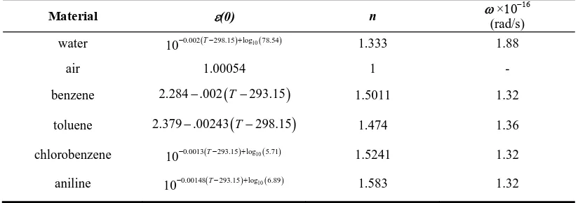
temperature dependencies, are provided in Table 1. The electrolyte concentrations

applied to determine the screening effects in aqueous films are provided in Table 2

along with the calculated effective and nonretarded Hamaker constants.

4. Critical Film Thickness Scaling Laws

For a given drainage velocity expression, the zeroth order growth constant provides

higher values of critical thickness than the first order growth constant [11]. Also, the

magnitude of the film thickness integral in equation (8) and hence the size of the

critical film thickness is inversely proportional to the thinning velocity. Therefore, by

combining the Reynolds thinning velocity (equation (1)) and the zeroth order growth

constant (equations (8) and (9)) with equations (6), (7), and (12), an upper bound of the

critical thickness is obtained. This combination of equations is identical to the theory of

Ivanov et al [2]. Previous solutions have been provided [11, 18] with reference to a

master curve, which reflects the self-similarity of the film rupture process and is a

necessary condition for a scaling law [24]. The master curve elucidates three

subdomains over the relevant parameter space whose boundaries are defined by the

curve by a continuum of three lines, one line for each subdomain, allows the critical

thickness to be estimated over the entire relevant parameter space by the following

scaling law (see the appendix for an alternate derivation of the basic form of the scaling

law).

( ) ( )

h =C h P (16)

* * *

,0

, , and

c t

h h P are dimensionless parameters defined as follows.

* 0 2 c c h h ζ

= (17)

1 4 2 * ,0 0 0,1 2 t A R h ζ πσ α ⎡ _{⎛ ⎞} ⎤ ⎢ ⎥ = ⎜_⎜ ⎟_⎟ ⎢ _{⎝ ⎠} ⎥ ⎣ ⎦ (18)

(

)

( )

A R R P

R

πσ ζ

−

= (19)

0,1

α is the first root of the Bessel function of first kind order zero and has a value of

2.4048. The scaling law constants C, x, and y in equation (16) are dependent on the

system of equations solved, the relevant master curve, as well as the subdomain in

which a solution is sought. For the system of equations describing the upper bound of

the critical thickness, the scaling law constants take on the values provided in Table 3.

The system of equations representing the upper bound scaling law is identical to the

model described by Ivanov et al [2] for stationary films with high concentrations of

surfactant when the disjoining pressure is represented as shown in equation (2). Ivanov

et al did not provide a general solution in the form of limiting equations, but did show

that the model predicted higher than actual critical thickness values for a series of

aniline films. Ivanov et al also did not report all of the physicochemical properties

necessary to obtain their results, making a quantitative comparison with the scaling

laws impossible.

In a similar manner, the scaling law for the lower bound of the critical film thickness

was determined. This was accomplished by combining the theoretical MTsR equation

(i.e., equations (3) and (4)) and the first order growth constant (equations (10) and (11))

with equations (6), (7), and (12). The resulting lower bound scaling law constants are

It has been shown that the semi-empirical MTsR equation provides more accurate

estimates of the film thinning velocity in the unstable period of a large variety of films

[19]. Therefore, combination of the semi-empirical MTsR equation (i.e., equations (3)

and (5)) and the zeroth order growth constant (equations (10) and (11)) with equations

(6), (7), and (12) may provide more accurate estimates of critical thickness. The scaling

law constants for the lower bound of the critical film thickness are provided in Table 5.

5. Discussion

The utility of the critical thickness scaling law and the associated constants reported

here can be tested by comparing the scaling law predictions with measurements

reported in the literature. To meet this objective, critical thickness values reported on a

variety of foam and emulsion films were collected [3-7, 25-27]. All of the aqueous

films contained sufficient electrolyte to suppress electrostatic repulsion and the

interfaces of all of the films were rendered tangentially immobile by the presence of

surfactant. The physicochemical properties used for each film in application of the

scaling law are provided in Tables 1 and 2. Upper and lower bounds of the critical

thickness were calculated using equation (16) with the corresponding constants

determined by the drainage pressure condition described in Tables 3 and 4,

respectively. Scaling law predictions of the critical thickness bounds in foam and

emulsion films using the effective Hamaker constant are compared to the

experimentally measured values in Figure 2 and 3. The results demonstrate that only a

portion of the foam and emulsion critical thickness measurements are bounded when

the effective form of the retarded Hamaker constant is used. For a given film system,

the scaling law predicts that the critical film thickness will increase with increasing film

radius. This is consistent with the measurements reported in the studies included here.

In Figure 2, it is shown that foam films of small radii are bounded by the scaling law

predictions whereas the larger films are not. In Figure 3, the no. 6 emulsion films (i.e.,

tolunen-water-toluene films) of Manev et al [6] are bounded while the other emulsion

films are not. The effective Hamaker constant appears to be within a suitable range for

smaller films but does not adequately represent the long range van der Waals attraction

It has recently been observed that long range van der Waals forces appear to have a

much larger effect in liquid films than is predicted by the retarded Hamaker constant

obtained from Lifshitz theory. Sharma et al [13] observed the breakup of micrometer

thick polydimethylsiloxane (PDMS) films on solid substrates over time periods that

were several orders of magnitude shorter than is predicted by thin film theory. Chen et

al [12] independently measured the separation distance at which PDMS or

polybutadiene films supported on mica substrates coalesce due to a jump instability

created by long range van der Waals attractrive forces. The jump-in distance was

measured at around 2000 Å, which is in agreement with theoretical predictions when

the non-retarded Hamaker constant is used to represent long range forces. It is therefore

of interest to determine if critical film thickness measurements reported in the literature

are more globally consistent with the scaling law predictions when the non-retarded

Hamaker constants provided in Table 2 are used. Scaling law predictions of the critical

thickness bounds in foam and emulsion films using the non-retarded Hamaker

constants are compared to the experimentally measured values in Figure 4 and 5. The

scaling law bounds are shown to be much more consistent with the experimental

measurements. In Figure 4, essentially all of the critical thickness measurements in the

foam films are bounded. Also, with the exception of system no. 1 of Traykov et al [3],

all of the emulsion films in Figure 5 are shown to be bounded by the scaling law

predictions. Emulsion film systems nos. 1 and 4 of Traykov et al contained the same

materials but were inverted. That is, film system no. 1 consisted of a benzene film

surrounded by water whereas film system no. 4 consisted of a water film surrounded by

benzene. According to Lifshitz theory, the Hamaker constants for these two systems are

equivalent which is consistent with the Hamaker constants shown in Table 2. However,

the critical film thickness measured in system no. 1 was about 35% thicker than in

system no. 4. This discrepancy can not be explained by the difference in interfacial

tension. The non-retarded Hamaker constant of system no. 4 would have to be

increased by a factor of 3 to obtain agreement with the scaling law predictions.

It is of interest to explore this approach when a more accurate film thinning model is

coupled with the corrugation growth equation. For this purpose, the semi-empirical

MTsR equation was coupled with the zeroth order corrugation growth constant and the

resulting scaling law constants are provided in Table 5. The scaling law predictions for

effective and non-retarded Hamaker constants are used, respectively. Here too,

predictions using the non-retarded Hamaker constant more accurately predict the

critical film thickness measurements.

6. Conclusions

It is shown in this study that the average critical film thickness of emulsion and foam

films can be bounded using a simple scaling law with the constants provided in Tables

3 and 4 when the non-retarded Hamaker constant is employed. The analysis

demonstrates general agreement between the predictions of spontaneous rupture theory

with the experimental measurements of a broad range of foam and emulsion films

based on the growth of the optimum waveform. The equations used in this study only

approximate the dynamics of film thinning and corrugation growth in thin films. The

scaling laws used to predict bounds for the critical thickness were obtained following a

quasi-static approach in which the fastest corrugation growth and slowest film thinning

models, or alternatively, the slowest corrugation growth and fastest film thinning

models were combined. Although the particular drainage and corrugation growth

models in the underlying equations influence the resulting critical thickness predictions,

the choice of drainage model appears to have the largest effect. When the scaling law

incorporating the more accurate semi-empirical MTsR drainage equation is used, the

resulting critical thickness predictions are more accurate for small to moderately sized

films. The scaling laws can also be applied to bound the Hamaker constant when

accurate critical thickness values are known.

7. Acknowledgements

This work was supported in part by the U. S. Department of Energy under contract

W-7405-ENG-36. The authors are grateful to a referee of the original manuscript, who

recommended the application of Lifshitz theory to determine the Hamaker constants.

8. Appendix

The basic form of the scaling law can be obtained by assuming that the drainage

pressure in equation (2) is dominated by either the Plateau border pressure drop or the

disjoining pressure term. Under conditions when the Plateau border pressure drop

equation (12) can be integrated directly. Substitution of equation (9) for k_opt provides the following equation relating the critical and transition thicknesses of the optimum

waveform.

4 3

6 c 7 c 1

t t h h h h ⎛ ⎞ ⎛ ⎞ = − ⎜ ⎟ ⎜ ⎟

⎝ ⎠ ⎝ ⎠ (A1)

Limiting the film thickness ratio to positive values less than 1 provides:

0.72

c t

h h

β = ≈ (A2)

Integration of the zeroth order corrugation growth constant given by equation (8)

followed by substitution of equation (9) provides:

(

)

2 2

0 2 4 3 3 4

,

1 1 1

16 3

t c

B t c t t

h h A R

X

P h_σ h h h

π σ

⎡ ⎛ ⎞ − ⎤

= _{⎢ ⎜} − _⎟− _⎥

⎢ ⎝ ⎠ ⎥

⎣ ⎦ (A3)

The transition thickness is eliminated by substitution of equation (A2).

(

)

2 2

3 4 4

0 2 7

,

1 4 3

48 _{B c}

A R X

P h_σ β β β

π σ

= − + (A4)

The zeroth order growth rate constant can be rearranged in the form of the

dimensionless constants defined in equations (17) through (19). Introducing the

resulting growth constant expression into equation (6) provides the following equation

for the dimensioless critical film thickness.

(

)( )

( )

4

2 4 3 4 * *

0,1 ,0

*

7 *

1 4 3

exp 8 t c c h P h h

α β β β

⎡ _{− +} ⎤ ⎢ ⎥ = ⎢ ⎥ ⎣ ⎦ (A5)

Taking the natural logarithm of both sides provides the basic form of the scaling law.

(

)

( )

( ) ( )

1 7

2 4 3 4

4 7 1 7 0,1

* * *

,0 *

1 4 3

8 ln

c t

c

h h P

h

α β β β

⎡ − + ⎤ ⎢ ⎥ = ⎢ ⎥ ⎣ ⎦ (A6)

The values of the exponents in equation (A6) are approximately equal to the x and y

values listed in the last row of Table 3. The quantity in the square brackets is slightly

dependent on the value of the dimensionless critical film thickness, which ranges

approximately between 10 and 100. This provides a C value that ranges between 0.54

and 0.60. The slightly larger C value provided in the last row of Table 3 compensates

A similar approach under conditions where the drainage pressure is dominated by the

disjoining pressure provides a β value of 0.67 and equation (A6) becomes:

(

)

( )

( )

1 4

2 4 4

0,1

* *

,0 *

1

ln 1

4 8 ln

c t

c

h h

h

α β β β

⎧₋ ⎡ _{+ −} ⎤⎫

⎪ ⎢ ⎥⎪

⎪ ⎣ ⎦⎪

= ⎨ ⎬

⎪ ⎪

⎪ ⎪

⎩ ⎭

(A7)

The value of the x parameter in the first row of Table 3 is smaller than unity. Although

the difference is small, it effectively reduces the value of the critical film thickness by

half. The difference is compensated for in the value of the C parameter. In equation

(A7), the value of C ranges between 0.25 and 0.33, which is about half of the value

provided in Table 3. The differences between the scaling law parameters provided in

this appendix and those in Table 3 are a consequence of the master curve approach

described in the previous scaling law section. The master curve approach yields

approximate values of the scaling law parameters across the entire range of drainage

pressure conditions as well as the approximate boundaries where the various forms of

the scaling law are applicable.

Rearrangement of the scaling law into a dimensional form provides an equation that is

similar in form to the limiting equations of Vrij [7, 26], which included an undefined

parameter (f) that was reported to be slightly dependent on film thickness.

9. References

1. I.B. Ivanov and D.S. Dimitrov, Thin Film Drainage, Marcel Dekker, Inc., 1988.

2. I.B. Ivanov, B. Radoev, E. Manev and A. Scheludko, Trans. Faraday Soc., 66

(1970) 1262

3. T.T. Traykov, E.D. Manev and I.B. Ivanov, International Journal of Multiphase

Flow, 3 (1977) 485

4. A.A. Rao, D.T. Wasan and E.D. Manev, Chem. Eng. Commun., 15 (1982) 63

5. B.P. Radoev, A.D. Scheludko and E.D. Manev, J. Colloid Interface Sci., 95 (1983)

254

6. E.D. Manev, S.V. Sazdanova and D.T. Wasan, J. Colloid Interface Sci., 97 (1984)

591

7. A. Vrij, Discuss. Faraday Soc., 42 (1966) 23

9. A. Sharma and E. Ruckenstein, Langmuir, 3 (1987) 760

10. A. Sheludko, Adv. Colloid Interface Sci., 1 (1967) 391

11. J.E. Coons, P.J. Halley, S.A. McGlashan and T. Tran-Cong, Adv. Colloid Interface

Sci., 105 (2003) 3

12. N. Chen, T. Kuhl, R. Tadmor, Q. Lin and J.N. Israelachvili, Physical Review

Letters, 92 (2004) 024501/1

13. A. Sharma, R. Khanna and G. Reiter, Colloids and Surfaces B: Biointerfaces, 14

(1999) 223

14. O. Reynolds, Philos. Trans. R. Soc. London, 177 (1886) 157

15. E. Manev, R. Tsekov and B. Radoev, J. Dispersion Sci. Technol., 18 (1997) 769

16. J.E. Coons, P.J. Halley, S.A. McGlashan and T. Tran-Cong, Drainage of Emulsion

and Foam Films in Scheludko Cells, 5th European Conference on Foams,

Emulsions and Applications, Champs-sur-Marne, France, July 2004.

17. J.E. Coons, P.J. Halley, S.A. McGlashan and T. Tran-Cong, Drainage of Emulsion

and Foam Films in Scheludko-Exerowa Cells, 21st International Congress of

Theoretical and Applied Mechanics, August 2004.

18. J.E. Coons, P.J. Halley, S.A. McGlashan, T. Tran-Cong and A.L. Graham,

Bounding the Critical Rupture Thickness of Common Thin Films, 14th

International Congress on Rheology, Seoul, Korea, August 2004.

19. J.E. Coons, P.J. Halley, S.A. McGlashan and T. Tran-Cong, Colloids and Surfaces

A: Physicochemical and Engineering Aspects, (Submitted 2004)

20. J.E. Coons, P.J. Halley, S.A. McGlashan, T. Tran-Cong and A.L. Graham,

Bounding the Critical Rupture Thickness of Common Thin Films, 5th European

Conference on Foams, Emulsions and Applications, Champs-sur-Marne, France,

July 2004.

21. R. Tsekov, Colloid Surf. A-Physicochem. Eng. Asp., 141 (1998) 161

22. W.B. Russel, D.A. Saville and W.R. Schowalter, Colloidal Dispersions,

Cambridge University Press, New York, 1989.

23. J.N. Israelachvili, Intermolecular and Surface Forces, Academic Press, San Diego,

1992.

24. G.I. Barnenblatt, Scaling, Cambridge University Press, Cambridge, United

Kingdom, 2003.

25. A. Vrij, Discuss. Faraday Soc., 42 (1966) 60

27. K. Kumar, A.D. Nikolov and D.T. Wasan, J. Colloid Interface Sci., 256 (2002)

194

28. R.C. Weast, Handbook of Chemistry and Physics, CRC Press, Inc., Baco Raton,

TABLES

Table 1. Dielectric and optical properties1 of reference film materials.

Material ε(0) n ω ×10

−16

(rad/s) water 0.002( 298.15)log10(78.54)

10− T− + 1.333 1.88

air 1.00054 1 - benzene 2.284 .002−

(

)

toluene 2.379 .00243−

(

)

aniline 0.00148( 293.15)log10(6.89)

10− T− + 1.583 1.32

1

( )

0

Table 2. Source of experimental data and the physicochemical properties used for the prediction of critical thickness.

Source of Data and Film Material

Film Type

20

4

10 3 hc

A ×

(Nm)

A(0)×1020

(Nm)

T

(ºC)

σ ×103

(N/m)

Rc

(μm)

R

(μm)

Vrij [7] air-aniline-air air-water-air Foam Foam2 2.7 1.7 6.5 3.6 253 253 39.4 65 18404 17904 100 100

Exerowa & Kolarov (see Vrij [7], page 60)

air-water-air Foam2 1.2-1.6 3.6 253 55.5 23104 100-400

Scheludko & Manev [26] air-chlorobenzene-air air-aniline-air Foam Foam 2.1-3.1 2.6-3.7 5.5 6.5 20 20 32.6 42.6 1140 1140 36-257 36-200

Traykov et al [3]

water-benzene-water (1) benzene-water-benzene (4) Emulsion Emulsion5 0.59 0.34 0.84 1.1 20 20 28 34 1350 1450 100 100

Rao et al [4]

air-water-air Foam6 1.5-1.7 3.6 25 35 1790 90-140

Radoev et al [5]

air-water-air

Foam6 0.86-1.9 3.6 24 34.5 17904 50-1000

Manev et al [6]

air-water-air (1) air-water-air (2) air-water-air (3) air-water-air (4) toluene-water-toluene (5) toluene-water-toluene (6) Foam6 Foam7 Foam7 Foam7 Emulsion5 Emulsion6 1.1-1.9 1.1-1.9 1.1-1.9 1.1-1.9 0.20-0.29 0.20-0.29 3.6 3.6 3.6 3.6 0.86 0.86 25 25 25 25 25 25 44.5 37.0 34.0 34.0 15.0 7.9 1790 1790 1790 1790 1580 1580 50-500 50-500 50-500 50-500 50-300 50-300

Kumar et al [27]

air-water-air Foam8 _{1.6 3.6 25 37.1 930 178}

2

Aqueous films contained 0.1M KCl.

3

The temperature was not reported by the data source so the value shown was assumed.

4

The capillary tube radius was not reported by the data source so the value shown was calculated from the Plateau border pressure drop.

5

Aqueous films contained 0.3M NaCl.

6

Aqueous films contained 0.1M NaCl.

7

Aqueous films contained 0.25M NaCl.

8

Table 3. Scaling Law Constants for the Upper Bound of the Critical Thickness

( )

* *

,0

t

z=P h Dominant Film Pressure

Term Throughout Drainage C x y

1.239

z> Disjoining pressure 0.514 0.944 0

1.239> >z 0.0190 Both disjoining pressure and

the Plateau border pressure 0.506 0.735 0.073

0.0190

Table 4. Scaling Law Constants for the Lower Bound of the Critical Thickness

( )

* *

,0

t

z=P h Dominant Film Pressure

Term Throughout Drainage C x y

1.994

z> Disjoining pressure 0.491 0.899 0

1.994> >z 0.0172 Both disjoining pressure and

the Plateau border pressure 0.448 0.535 0.133

0.0172

Table 5. Scaling Law Constants for Intermediate Critical Thickness Values

( )

* *

,0

t

z=P h Dominant Film Pressure

Term Throughout Drainage C x y

1.994

z> Disjoining pressure 0.523 0.920 0

1.994> >z 0.0172 Both disjoining pressure and

the Plateau border pressure 0.476 0.563 0.133

0.0172

FIGURE CAPTIONS

Figure 1. The contribution of the film thickness dependency of the retarded Hamaker constant to the effective Hamaker constant as predicted by Lifshitz theory. The value of the bracketed term is shown for benzene, aniline, chlorobenzene, and aqueous films as a function of the film thickness. The contribution is mostly dependent on the film material and not on the material of the surrounding medium. The thickness dependence of benzene films is almost negligible while the contribution in films of the other materials is particularly high when the film thickness is around 1000 Å.

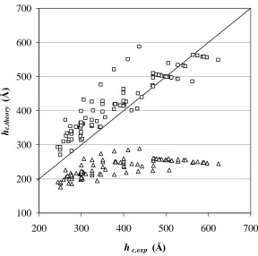
Figure 2. The critical rupture thickness bounds of foam films determined using the effective Hamaker constants in Table 2. The upper (□) and lower (∆) bounds were determined by the scaling law with constants from Tables 3 and 4, respectively. The size of the critical thickness increases approximately with increasing film radius. Critical film thickness measurements in the smaller films are bounded by the scaling law predictions whereas those in the larger films are not bounded.

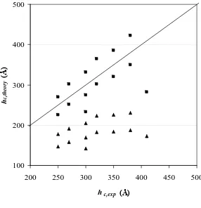
Figure 3. The critical rupture thickness bounds of emulsion films determined using the effective Hamaker constants in Table 2. The upper (■) and lower (▲) bounds were determined by the scaling law with constants from Tables 3 and 4, respectively. The size of the critical thickness approximately increases with increasing film radius. Critical film thickness measurements of system no. 6 in Manev et al [6] is the only emulsion film system sufficiently bounded.

Figure 4. The critical rupture thickness bounds of foam films determined using the non-retarded Hamaker constants in Table 2. The upper (□) and lower (∆) bounds were determined by the scaling law with constants from Tables 3 and 4, respectively. The size of the critical thickness

approximately increases with increasing film radius. Critical film thickness measurements over the entire range are bounded by the scaling law predictions.

Figure 5. The critical rupture thickness bounds of emulsion films determined using the non-retarded Hamaker constants in Table 2. The upper (■) and lower (▲) bounds were determined by the scaling law with constants from Tables 3 and 4, respectively. The size of the critical thickness approximately increases with increasing film radius. Critical film thickness measurements for all of the emulsion films are bounded except for system no. 1 emulsion of Traykov et al [3].

Figure 6. The critical rupture thickness of emulsion (■) and foam (□) films determined using the effective Hamaker constants in Table 2 along with the scaling law constants of Table 5. The theoretical values are significantly lower than the experimental measurements.

FIGURES

Figure 1.

-1.2 -1 -0.8 -0.6 -0.4 -0.2 0

100 1000 10000

h (A)

Benzene

Aniline and Chlorobenzene

Figure 2.

100 200 300 400 500 600 700

200 300 400 500 600 700

hc,exp (Å)

h

c,

th

eo

ry

(Å

Figure 3.

100 200 300 400 500

200 250 300 350 400 450 500

hc,exp (Å) hc,

th

eo

ry

(Å

Figure 4.

200 300 400 500 600 700 800 900

200 300 400 500 600 700

hc,exp (Å)

h

c,

th

eo

ry

(Å

Figure 5.

100 200 300 400 500 600

200 250 300 350 400 450 500

hc,exp (Å) hc,

th

eo

ry

(Å

Figure 6.

100 200 300 400 500 600 700

200 300 400 500 600 700

hc,exp (Å) hc,

th

eo

ry

(Å

Figure 7.

200 300 400 500 600 700

200 300 400 500 600 700

hc,exp (Å) hc,

th

eo

ry

(Å