The structure and dynamics of spawning aggregations of coral reef fish

Full text

(1)88. CHAPTER 4: SPAWNING AGGREGATION SITES: PHYSICAL AND BIOTIC CHARACTERISTICS 4.1. Introduction A large number of marine species migrate prior to breeding. For many of these species, such migrations are necessary because suitable habitat in which to breed is not found in the species’ feeding areas. These species include, turtles which feed in the sea but need to lay eggs on sandy beaches (Hendrickson 1980), anadromous fishes which must return from the sea to lay eggs in freshwater streams (Klemesten et al. 2003), and the Christmas Island red crab which migrates across land to release eggs in the sea (Adamczewska & Morris 2001). Such migrations are essential for their offspring’s survival. However, for other species, breeding migrations are less easily explained in terms of the spatial separation of breeding and feeding habitat. Spawning aggregations are known to be formed by a number of coral reef fish, most of which spawn pelagically (see Claydon 2004). Water into which eggs are spawned is not limited, yet some individuals have been documented migrating over 100km to spawn in aggregations at certain locations and times (Colin 1992, Carter et al. 1994, Bolden 2000). It seems unlikely that effective reproduction necessitates such migrations, because a host of pelagically spawning coral reef animals, both vertebrate and invertebrate, do not and/or cannot migrate prior to spawning (e.g. some species of reef fish, Donaldson 1989; Popper & Fishelson 1973; sponges, Fell 1974; and corals, Willis et al. 1985).. It is often suggested that the sites where pelagic spawning occurs have characteristics that are intrinsically beneficial to the individuals spawning (e.g. Thresher 1984, Donaldson 1990, Shapiro et al. 1993, Whaylen et al. 2004). Such assertions are unsurprising, particularly in the context of spawning aggregation formation: the site represents a choice made from a sometimes very large area of reef (e.g. Epinephelus striatus, Colin 1992, Carter et al. 1994, Bolden 2000); this choice seldom appears to be arbitrary because such sites are typically perceived to have distinctive characteristics (not necessarily correctly, see Domeier et al. 2002, Claydon 2004), and the same choice can be made by very large numbers of conspecifics (over 100,000, Smith 1972) as well as by several other species,.

(2) 89 forming spawning aggregations at the same site (Moyer 1989, Colin & Bell 1991, Carter et al. 1994, Johannes et al. 1999, Sancho et al. 2000b, Domeier et al. 2002, Whaylen et al. 2004). The more conspecifics and the greater number of species that choose the same site, the more convincing this assertion becomes. Despite being rarely documented, more than 10 species spawning aggregatively at the same site is likely to be common for both relatively small species (Sancho et al. 2000b), and larger predatory species (Whaylen et al. 2004). As many as 60 species of both types of reef fish have been documented spawning at the same site (Johannes et al. 1999). Whilst this observation may include a misleadingly elevated number of smaller species because of the inappropriately large spatial scale over which it was made, 27 species have been observed forming spawning aggregations at a site less than 10 x 10m on a reef in Papua New Guinea (see Chapter 2).. The physical characteristics of these sites are proposed to enhance the survival of spawning adults and their eggs by means of a number of mechanisms: (1) the geomorphology and topography of the sites limit the foraging efficiency of piscivores and offer abundant refuge to prey (Shapiro et al. 1988, Hugie & Dill 1994), (2) the geomorphology of sites facilitates the rapid removal of eggs away from the reef into deeper less planktivore-rich waters (Johannes 1978), and (3) the currents found at these sites enhance this off-reef egg transport (Robertson & Hoffman 1977, Johannes 1978) and may facilitate the future recruitment of larvae back onto reefs (Lobel 1978, Barlow 1981). These sites are also proposed to have characteristically lower abundances of potential predators of both spawning adults and their planktonic eggs (Johannes 1978). There are two reef features that may facilitate the more rapid removal of eggs away from planktivores: horizontal seaward projections and steep slopes. In a random current regime, the further a point on a reef projects out to sea the more likely currents at that point flow directly away from the reef. The steeper the reef slope the less time it takes for eggs to be swept into deeper less planktivore-rich waters. Therefore, eggs spawned from sites with these two features will be less exposed to reef-associated planktivores than those spawned from straighter margins of reef with shallow inclining reef slopes..

(3) 90 The physical characteristics of spawning aggregation sites are seldom described in less than ambiguous terms. This ambiguity reinforces the perception that spawning aggregations form at sites with distinctive characteristics. However, when all reef formations are likely to be characterized by only a few categories (e.g. slope, wall, promontory, channel, seaward projection), the distinctiveness of such characteristics is questionable (see Claydon 2004). Even if sites were adequately described, it is necessary to describe many such sites and compare these to sites where spawning aggregations are not formed. Almost without exception, spawning aggregations are documented without detailed reference to surrounding areas of reef. Therefore, it is usually impossible to ascertain the range from which a choice of sites was made, and there is little quantitative support that the choice of sites for spawning aggregation formation enhances the survival of adults or their offspring.. 4.1.1 Aims: The aims of this study are to investigate whether spawning aggregations of coral reef fish are formed at characteristic locations and with regard to physical and biological parameters. Specifically, this study will test the prediction that spawning aggregations are formed at locations and times where the physical and biological characteristics serve to reduce predation on eggs and adults. The physical characteristics investigated are both the broad-scale measurements of reef slope and the degree to which the reef margin projects seawards, as well as measurements taken on a finer scale: potential refuge from predators as indicated by topographic complexity and the number of holes in the substratum. Currents are treated comprehensively in a separate study (see Chapter 5). The biological characteristics of interest are the abundance and activities of piscivorous and planktivorous predators..

(4) THE IMAGES ON THIS PAGE HAVE BEEN REMOVED DUE TO COPYRIGHT RESTRICTIONS.

(5) 92. 4.2 Materials and Methods: 4.2.1 Study species: The “lined bristletooth” surgeonfish, Ctenochaetus striatus (max S.L. 16cm), was observed forming spawning aggregations with up to 2000 individuals on the inshore study reefs of Kimbe Bay. Study of aggregative spawning in this species was facilitated by the fact that: (1) spawning aggregations were consistently formed at specific sites on reefs, (2) many reefs had a number of such spawning sites, and (3) spawning occurred within a 2hour site-specific time window.. 4.2.2 Study area and study sites: Fieldwork was conducted from the Mahonia na Dari Research and Conservation Centre, Kimbe Bay, West New Britain Province, Papua New Guinea. The study focused on 4 inshore reefs in Kimbe Bay: Hanging Gardens, Kume, Limuka and Maya’s (see Figure 4.1). These reefs are characterised by shallow reef flats (1m at high tide) that are exposed at extreme low tides, and all margins of reef descend rapidly to over 20m down steep reef slopes or vertical walls. Reefs are separated by depths of over 50m. The broad-scale physical characteristics (the degree to which the reef projected seawards and the incline of the reef slope) were calculated from aerial photographs of the 4 reefs taken in 2004. The biotic and fine-scale physical characteristics were measured at 6 sites each on Hanging Gardens, Maya’s and Limuka (see Figure 4.1). At least 2 sites on each reef were known to be locations where Ctenochaetus striatus formed spawning aggregations (Hanging Gardens Sites 1,3 & 6, Maya’s Sites 1 & 4, Limuka Sites 1,2,3 & 5), and at least 2 sites were known to be locations where no such aggregations were formed (Hanging Gardens Sites 2, 4, & 5, Maya’s Sites 2,3,5 & 6, and Limuka Sites 4 & 6). The latter sites cannot be regarded as random because they were preferentially chosen from margins of reef with prominent seaward projections (a feature shown in this study to be characteristic of C. striatus spawning aggregation sites; see results). If no such areas of reef were available, then sites were chosen randomly from the remainder of the reef..

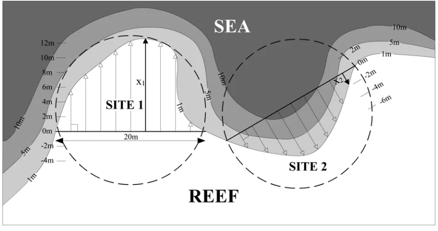
(6) 93 4.2.3 Broad-scale physical characteristics: The degree to which the reef projected in a seaward direction was calculated from aerial photographs of the reefs. Sections 20m long were taken across the 1m depth contour so that each end of the section lay on the contour. The scale of the sections was set at 20m because smaller sections also failed to identify seaward projections, and larger sections were not appropriate to the spatial scale of spawning aggregation formation. The 1m depth contour was used because this was the depth at which Ctenochaetus striatus formed spawning aggregations. The distance of the 1m contour perpendicular to this section was calculated at 2m intervals (excluding the 2 end points of the section). This distance was negative if the 1m contour bent back towards the reef in a concave manner, and positive if projecting seawards. The maximum distance for each site was obtained from these 9 measurements (see Figure 4.2). The maximum seaward projection was calculated at all known C. striatus spawning aggregation sites on Hanging Gardens, Kume, Limuka and Maya’s reefs. The remainder of each reef was divided up into 20m sections along the 1m depth contour and maximum seaward projection was calculated perpendicular to all of these additional sections. Measurements were not taken on the back reef area of Kume (the south-western margin from Site 1 to Site 16; see Figure 4.1) because searches for spawning aggregations of C. striatus were not performed on this section of reef. For each section, the maximum seaward projection was the measure chosen rather than the mean of the 9 measurements because the latter failed to identify many seaward projections. The reef slope was measured on 2 scales: the slope from 1m to 5m, and 1m to 10m. Measurements were taken from the 1m, 5m and 10m depth contours estimated from aerial photographs of Hanging Gardens, Kume, Limuka, and Maya’s reefs, and the slope was calculated by means of trigonometry. The maximum slope (closest to vertical) was calculated at the two end points of each 20m section used for the maximum seaward projection measurements and at 9 additional points along the 1m contour within the section. In this way the mean slope was calculated both at 1 to 5m and 1 to 10m at all Ctenochaetus striatus spawning aggregation sites and at all other margins of all 4 reefs (except the back reef of Kume; see above)..

(7) 94. Figure 4.2. Measurement of maximum seaward projection at convex (Site 1) and concave (Site 2) areas of reef. x1 = maximum seaward projection at Site 1; x2 = maximum seaward projection at Site 2.. 4.2.4 Fine-scale physical and biotic characteristics: At each of the 6 sites on Hanging Gardens, Limuka and Maya’s, the potential refuge from pisicvorous predators afforded to Ctenochaetus striatus by the substratum was measured along 4 randomly placed 10 m long transects. 10m long transects were chosen because this was the maximum length that could be used whilst still exclusively representing the site in question. Potential refuge from predation was measured directly by counting the number of holes lying under each transect line. Holes were counted only if they were of a size that could be used by C. striatus as shelter whilst also being too small for piscivores to enter (holes of a maximum diameter between 6 to 20cm). Potential refuge was also estimated indirectly from a measure of topographic complexity. Topographic complexity was measured using the contoured vs. linear length (“chain and tape”) method (Risk 1972).. 4.2.5 Piscivorous and planktivorous fishes: The abundance of piscivorous and planktivorous fishes was measured at sites in order to investigate whether the densities of predatory fishes (both of spawning adults and eggs).

(8) 95 were reduced at sites and times where and when Ctenochaetus striatus formed spawning aggregations. This was achieved by recording all fishes found within a radius of 5m from a fixed point in each site during a 2 minute interval, categorising fish seen as: spawners, piscivores, planktivores, and egg predators. Piscivores of interest were those deemed capable of preying upon C. striatus (carangids, carcharhinids, lutjanids, scombrids, and serranids >30cm S.L.). Because of the low densities of piscivores, their presence was further established by means of a timed (3 minute) swim around each site recording piscivores up to a depth of 7.5m. Planktivorous fishes were further categorised as those that consumed eggs within seconds of being spawned whilst the gamete cloud was still visible by targeting the apex of spawning rushes, hereafter referred to as target egg predators, and those that did not. On any given day, data were collected at a single reef, moving round the reef from one site to the next from early afternoon until sunset. In this fashion a record of the assemblage of planktivorous and piscivorous fishes was established for each site at varying times in the afternoon. This was necessary because the abundance and activity of piscivores and planktivores is known to vary throughout the day (Hobson 1974, 1975, Hobson & Chess 1978, Danilowicz & Sale 1999). For sites where C. striatus formed spawning aggregations, the assemblage of fishes within sites was established at both times of aggregative spawning and at times of no such spawning. The wet weight biomass of planktivores was estimated by length-weight relationships in Froese and Pauly (2000). The estimate of wet weight biomass gave a measure of planktivory that could be compared between sites and times. Data were collected over 27 days at Hanging Gardens, 19 days at Limuka and 31 days at Maya’s, and represent over 300hrs of observations spread over days in March, April, May, October and November in 2003.. 4.2.6 Data analyses: Seaward projection and slope- Data from each reef were treated separately. Student’s ttests were used to compare means from spawning aggregation sites with means from non spawning aggregation sites within a reef for maximum seaward projection and for incline of reef slope data (both 1 to 5m and 1 to 10m). Williams corrected goodness of fit G-tests.

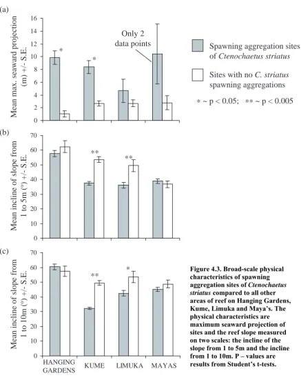
(9) 96 were used to test whether spawning aggregations were formed at sites on Kume with greater seaward projection at a significantly higher frequency than that predicted by a random distribution of sites. Such G-tests could not be performed on data from other reefs because there were too few spawning aggregation sites for analyses (expected frequencies were too low; Sokal & Rohlf 1995). Fine-scale physical, piscivore and planktivore data- For each reef, separate 2-factor oneway ANOVA’s were used to compare topographic index, number of holes, planktivore biomass, target egg predator biomass, and piscivore abundance. Factors were (1) spawning aggregation site vs. site where no aggregation formed, and (2) site. Student’s ttests were used to compare planktivore biomass, target egg predator biomass, and piscivore abundance at times of spawning aggregation formation and at other times within spawning aggregation sites. STATISTICA 6 statistics package was used for ANOVA and t-test analyses. Zar (1999) χ2 tables were consulted for p-values of G-tests. α-levels for all analyses were 0.05.. 4.3 Results: 4.3.1 Seaward projection of reef margin: All sites where Ctenochaetus striatus formed spawning aggregations were found on areas of reef that projected seawards (i.e. all sites were on convex margins of reef). On all reefs spawning aggregations were formed at sites where the reef margin projected further seawards than other areas of reef (see Figure 4.3). However, this relationship was only significant at two of the four reefs, with Maya’s having insufficient data for analysis (see Figure 4.3 and Table 4.1). Not all prominent seaward projections were used as spawning aggregation sites: areas of reef where spawning aggregations were not formed included sites where the reef margin projected further seawards than at some of the spawning aggregation sites. However, on Kume spawning aggregations were formed at sites with greater seaward projection at a significantly higher frequency than that predicted by a random distribution of sites (Williams corrected goodness of fit G-test: Gadj = 17.26, df =.

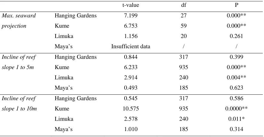
(10) 97 1, p < 0.001). Such G-tests could not be performed on data from other reefs because there were too few spawning aggregation sites for analyses (expected frequencies were too low; Sokal & Rohlf 1995).. Mean max. seaward projection (m) +/- S.E.. (a) 16 14. Only 2 data points. 12 10. Spawning aggregation sites of Ctenochaetus striatus. * *. 8. Sites with no C. striatus spawning aggregations. 6 4. * ~ p < 0.05; ** ~ p < 0.005. 2 0. (b) Mean incline of slope from 1 to 5m (o) +/- S.E.. 70 60. **. 50. **. 40 30 20 10 0. (c) Mean incline of slope from 1 to 10m (o) +/- S.E.. 70 60. **. 50. *. 40 30 20 10 0. HANGING GARDENS. KUME. LIMUKA. MAYAS. Figure 4.3. Broad-scale physical characteristics of spawning aggregation sites of Ctenochaetus striatus compared to all other areas of reef on Hanging Gardens, Kume, Limuka and Maya’s. The physical characteristics are maximum seaward projection of sites and the reef slope measured on two scales: the incline of the slope from 1 to 5m and the incline from 1 to 10m. P – values are results from Student’s t-tests..

(11) 98 4.3.2 Reef slope: The incline of the reef slope ranged from 3 to 90o and 5 to 90o (shallow incline to vertical drop) at scales of 1 to 5m and 1 to 10m respectively. However, despite a hypothetical enhancement to the survival of eggs spawned from areas of reef with steeper reef slopes, spawning aggregations were not formed exclusively at such locations: at Kume and Limuka spawning aggregation sites were found on margins of reef with significantly less steep slopes than the other areas of reef, whilst on Hanging Gardens and Maya’s there were no significant differences (see Figure 4.3 and Table 4.1).. Table 4.1. Broad-scale physical data: results of Student’s t-tests between spawning aggregation sites and all other sites on reefs for maximum seaward projection of sites, incline of reef slope from 1 to 5m, and incline of reef slope from 1 to 10m. *~ p < 0.05; **~ p < 0.005. t-value. df. P. Max. seaward. Hanging Gardens. 7.199. 27. 0.000**. projection. Kume. 6.753. 59. 0.000**. Limuka. 1.156. 20. 0.261. Maya’s. Insufficient data. /. /. Incline of reef. Hanging Gardens. 0.844. 317. 0.399. slope 1 to 5m. Kume. 6.233. 935. 0.000**. Limuka. 2.914. 240. 0.004**. Maya’s. 0.493. 185. 0.623. Incline of reef. Hanging Gardens. 0.545. 317. 0.586. slope 1 to 10m. Kume. 10.575. 935. 0.0000**. Limuka. 2.578. 240. 0.011*. Maya’s. 1.010. 185. 0.314.

(12) Number of holes Topography. 12 ** 10 8 6 4 2 0 1 **. 6 ** 4 2 0 1 **. 0.5. 0.5. 0. Site:. 1. 2. 3. 4. 5. 6. HANGING GARDENS. 0. 8 **. 8. 6. 6. 4. 4. 2. 2. 0 1. 0 1. **. 0.5. 1. 2. 3. 4. LIMUKA. Spawning aggregation sites of Ctenochaetus striatus. 5. 6. 0. 0.5. 1. 2. 3. 4. 5. 6. 0. MAYAS Sites with no C. striatus spawning aggregations. FSAS NON. FSAS NON. FSAS NON. HANGING GDNS. LIMUKA. MAYAS. * ~ p < 0.05 **~ p < 0.005. Figure 4.4. The mean number of holes in the substratum (between 6 and 20 cm maximum aperture), and topographic complexity (Topography; 1 = flat, <1 =topographically complex) +/- S.E. at all 6 sites on Hanging Gardens, Limuka and Maya's. The means for all spawning aggregation sites (FSAS) vs. sites where spawning aggregations are not formed (NON) are also shown. P - values are the resultant probabilities from one-way ANOVA's.. 99.

(13) # Piscivores. 6 **. Planktivore biomass. **. 4 0.5. 0.5. 1. 0. 0. 0. 4. 4. 3. 3. 2. 2. 2 0. Egg pred biomass. 2. 1 **. 1 *. 4. **. 3 2. 6. **. 4. 1. 2. 1. 1. 0 4 **. 0 6 ** 5. 0. 0. 3. 3. 2. 2. 1. 1. 3 2 1 0. Site: 1 2 3 4 5 6 HANGING GARDENS. 3 2 1 1. *. **. ** *. 4. 0. **. 2. 3. 4. LIMUKA. Spawning aggregation sites of Ctenochaetus striatus. 5. 6. 0. 1. 2. 3. 4. 5. 6. 0. MAYA'S Sites with no C. striatus spawning aggregations. **. FSAS NON. FSAS NON. FSAS NON. HANGING GDNS. LIMUKA. MAYA'S. * ~ p < 0.05 **~ p < 0.005. 100. Figure 4.5. The piscivore presence (number of individuals) and planktivore biomass (kg) at study sites: the abundance of piscivores (>30cm S.L.), the estimated biomass of all planktivores, and the estimated biomass of target egg predators (Egg pred) at all sites on Hanging Gardens, Limuka and Maya's, and the means for all spawning aggregation sites (FSAS) vs. sites where spawning aggregations are not formed (NON) are also shown. All values are means +/- S.E. P - values are the resultant probabilities from one-way ANOVA's..

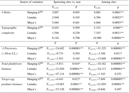
(14) 101 Table 4.2. Results of one-way ANOVA’s comparing number of holes, topographic complexity, number of piscivores (>30cm S.L.), total planktivore biomass, and target egg predator biomass between spawning aggregation sites and other sites (spawning sites vs. non) within reefs, and between all 6 sites on the reef (among sites). * ~ p < 0.05; ** ~ p < 0.005. Source of variation:. Spawning sites vs. non. Among sites. F(1,18). P. F(4,18). p. Hanging Gdns. 3.097. 0.095. 9.083. 0.0001**. Limuka. 2.948. 0.103. 6.396. 0.0022**. Maya’s. 5.684. 0.461. 4.666. 0.0093**. Topographic. Hanging Gdns. 0.454. 0.509. 5.153. 0.006**. complexity. Limuka. 1.546. 0.230. 7.343. 0.0011**. Maya’s. 0.144. 0.708. 16.980. 0.00001**. F. P. F. p. F(1,317) =24.692. 0.000001**. F(4,317) =51.325. 0.000001**. F(1,172) =0.731. 0.394. F(4,172) =3.346. 0.011*. F(1,461) =1.931. 0.165. F(4,461) =13.040. 0.000001**. F(1,317) =5.811. 0.016*. F(4,317) =10.162. 0.000001**. F(1,172) =21.026. 0.00001**. F(4,172) =24.113. 0.000001**. F(1,461) =47.114. 0.000001**. F(4,461) =1.343. 0.253. F(1,317) =6.441. 0.012*. F(4,317) =7.849. 0.000005**. # Holes. # Piscivores. Hanging G. (>30cm S.L.). Limuka. dns. Maya’s Total planktivore. Hanging G. biomass. Limuka. dns. Maya’s dns. Target egg. Hanging G. predator biomass. Limuka. F(1,172) =15.063. 0.0001**. F(4,172) =21.059. 0.00001**. Maya’s. F(1,461) =53.158. 0.000001**. F(4,461) =0.846. 0.497. 4.3.3 Refuge from predation: The potential refuge from predation afforded to Ctenochaetus striatus by the substratum at sites, as estimated by number of size-specific holes and topographic complexity, varied significantly between sites within reefs (see Figure 4.4 and Table 4.2). However, the choice of spawning aggregation sites did not appear to take advantage of refuge from piscivores: on all three reefs, there was no significant difference between the number of holes in the reef nor the topographic complexity between sites where spawning aggregations were formed and those not home to such aggregations (see Figure 4.4 and Table 4.2)..

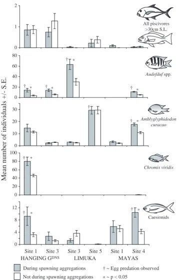
(15) 102 4.3.4 Piscivores: The piscivores >30 cm S.L. observed included species of Carcharinidae, Carangidae, Lethrinidae, Lutjanidae, and Serranidae. The abundance of these piscivores was generally low, with 6 out of 18 sites having a complete absence of piscivores >30cm S.L. (see Figure 4.5). It is unlikely that piscivores are maintained at an artificially low level by fishing pressure: although artisanal fishing occurs, this is at very low intensities, and fishing is prohibited altogether on Limuka. However, due to the nature of cryptic piscivores, it is likely their presence was underestimated especially at crepuscular times. Not one predatory attack on Ctenochaetus striatus was witnessed during observations that spanned over 1000hrs and include over 10,000 separate spawns of C. striatus. The only successful predatory attacks on any species occurred when two lutjanids attacked a bait ball (high-density school of several 1000 baitfish). Piscivores swam through sites on only 21 occasions. These predators were exclusively carangids (90.5%) and scombrids (9.5%), and on all but 2 occasions they swam through and disrupted spawning aggregations of C. striatus. On the 2 remaining occasions the spawning activities of labrids (Cheilinus trilobata, Epibulis insidiator) and a scarid (Chlororus bleekeri) were interrupted. Although potential prey sought refuge within the reef or advanced closer to it, the piscivores swam through sites at speeds well below that which would be considered a predatory attack. Such behaviour occurred significantly more often during spawning aggregations of C. striatus than predicted by sampling effort alone (Williams corrected G-test: Gadj = 41.6, df = 1, p < 0.001). However, the mean abundance of piscivores at spawning aggregation sites was only significantly greater than the mean at other sites on one reef, Hanging Gardens (see Figure 4.5 and Table 4.2). Furthermore, there were no significant differences between the abundance of piscivores at times of spawning aggregation formation than at other times at any of the spawning aggregation sites on any of the 3 reefs (see Table 4.3 and see Figure 4.6)..

(16) 103 2. All piscivores >30cm S.L.. 1. 0 80. † *. Mean number of individuals +/- S.E.. 60. Audefduf spp.. 40 20. † *. † *. † *. 0. †. 30. † * Amblyglyphidodon. 20. curacao. 10 0 100 80. † * Chromis viridis. 60 40 20 0 12. † *. † *. Caesionids. 8 4 0. Site 1 Site 3 HANGING GDNS. Site 3 Site 5 LIMUKA. During spawning aggregations. Site 1 Site 4 MAYAS † ~ Egg predation observed. * ~ p < 0.05 Figure 4.6. The abundance of piscivores and target egg predators at spawning aggregation sites at times when spawning aggregations are formed and at times when they are not. Only piscivores >30cm S.L. were included. Target egg predators illustrated are Abudefduf spp., Amblyglyphidodon curacao, Chromis viridis, and caesionids. Only sites with sufficient observations during spawning aggregations were included. P-values are the results of Student's t-tests between the abundance at times of spawning aggregation formation and abundance at other times. Not during spawning aggregations.

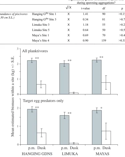
(17) 104 Table 4.3. The response of piscivores (>30 cm S.L.) to spawning aggregation formation. t-values and p-values are results of Student’s t-tests between mean abundance piscivores during spawning aggregations and at other times within the site. Only spawning aggregation sites with sufficient data were included. Significantly greater abundance of piscivores during spawning aggregations?. Abundance of piscivores (>30 cm S.L.). Mean estimated biomass within a site (kg) +/- S.E.. 3. √ /X. t-value. df. p. Site 1. X. 1.41. 90. >0.15. Hanging Gdns Site 3. X. 0.34. 81. >0.7. Limuka Site 3. X. 1.18. 55. >0.2. Limuka Site 5. X. 0.64. 50. >0.5. Maya’s Site 1. X. 0.69. 70. >0.4. Maya’s Site 4. X. 0.90. 159. >0.35. dns. Hanging G. All planktivores **. **. 2. **. 1. 0. Target egg predators only 2. **. * **. 1. 0. p.m. Dusk HANGING GDNS. p.m. Dusk LIMUKA. p.m. Dusk MAYAS. Figure 4.7. Mean estimated biomass of all planktivores and target egg predators only at times in the afternoon (p.m.) and at dusk (17:45 – 18:20 hrs). Means derived from data from all sites within reefs. * ~ p < 0.05; **~ p < 0.005. p – values are results of Student’s t-tests between mean biomass in the afternoon and mean at dusk..

(18) 105 4.3.5 Planktivores: Several species of planktivore were observed consumed eggs within seconds of being spawned by targeting the apex of Ctenochaetus striatus spawning rushes whilst gamete clouds were still visible (see Table 4.4 for list of target egg predators). The relative number of spawns attacked by these target egg predators was too difficult to quantify because of the rapid succession of spawns (>10 sec-1) within a small area and often large numbers of fishes feeding on eggs. However, target egg predation was observed during every spawning aggregation of C. striatus. Unlike pelagic spawning reef fish from other families which were observed delaying spawning in the presence of target egg predators or chasing them away, C. striatus continued spawning despite heavy losses of eggs. In this way C. striatus released eggs within cms of awaiting target egg predators. The estimated biomass of planktivores and target egg predators was significantly higher on all reefs at times in the afternoon compared to dusk (between 17:45 and 18:20hrs; see Figure 4.7 and Table 4.5). However, aggregative spawning of Ctenochaetus striatus was only witnessed once during this period, with all other spawning occurring during the more planktivore-rich times in the afternoon. The potential threat to eggs posed by planktivores appears to be greater at spawning aggregation sites than at alternative sites on reefs: on all three reefs the estimated biomass of planktivores in general and the biomass of species known to be target egg predators were significantly greater at spawning aggregation sites (see Figure 4.4 and Table 4.2). Additionally, some species of target egg predator appear to be attracted to spawning aggregations of Ctenochaetus striatus, moving from locations outside the sampling area to feed on spawned eggs: with the exception of sites where Abudefduf spp. were never seen, the mean abundances of Abudefduf spp. were significantly higher at times when spawning aggregations were formed than at other times within all spawning aggregation sites for which sufficient data were available for analyses (see Figure 4.6 and Table 4.6). Whenever C. striatus spawned, all Abudefduf spp. within the sampling area fed exclusively above the aggregation of surgeonfish. No other species of target egg predator displayed such a strong behavioural response to C. striatus spawning: despite being.

(19) 106 present at sites during aggregative spawning, Chromis viridis, Amblyglyphidodon curacao, and species of caesionid were not always observed feeding on spawned eggs. Furthermore, these egg predators were not observed feeding on spawned eggs in all C. striatus spawning aggregation sites in which they were found (see Figure 4.6 and Table 4.6). However, with only one exception, these egg predators were found in significantly higher numbers during C. striatus spawning aggregations at all sites in which they were observed feeding on C. striatus eggs (see Figure 4.6 and Table 4.6). The only exception to this was A. curacao at Limuka Site 5. Nonetheless, A. curacao also appeared to be attracted to this spawning aggregation. The data do not reflect this because the spawning aggregation was so large (over 1000 individuals) that most of it lay outside of the sampling area and individuals attracted to the aggregation were also found outside the sampling area..

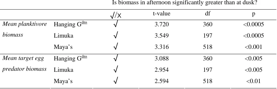
(20) 107 Table 4.4. Species observed feeding on eggs spawned by Ctenochaetus striatus on the inshore reefs of Kimbe Bay. Family. Genus. Species. Balistidae. Melichthys. vidua. Caesionidae. Unidentified spp.. (>10cm S.L.). Labridae. Thalassoma. hardwicke. Thalassoma. lunare. Lutjanidae. Macolor. niger (juvenile). Pomacentridae. Abudefduf. unidentified spp.. Acanthochromis. polyacanthus. Amblyglyphidodon. curacao. Amblyglyphidodon. leucogaster. Chromis. viridis. Rastrelliger. kanagurta. Scombridae. Table 4.5. The results of Student’s t-tests between the mean biomass of planktivores and target egg predators at times in the afternoon and at dusk (17:45 – 18:20hrs). Is biomass in afternoon significantly greater than at dusk?. Mean planktivore. Hanging G. biomass. Limuka. dns. Maya’s. √ /X √ √ √. t-value. df. p. 3.720. 360. <0.0005. 3.549. 197. <0.0005. 3.316. 518. <0.001. Mean target egg. Hanging Gdns. √. 3.088. 360. <0.005. predator biomass. Limuka. √ √. 2.954. 197. <0.005. 2.594. 518. <0.01. Maya’s.

(21) 108 Table 4.6. Feeding responses of target egg predators, Abudefduf spp., Amblyglyphidodon curacao, Chromis viridis and species of caesionid, to spawning aggregations of Ctenochaetus striatus. Only sites where egg predators were present are included. Egg predn ~ feeding on spawns of C. striatus observed at site; t-value and p-values are results of Student’s t-tests between mean abundance of egg predators during spawning aggregations and at other times within the site. Only spawning aggregation sites with sufficient data were included. † ~ significantly less egg predators during spawning aggregations. Egg predn? Abudefduf spp.. √ /X √ √ √ √. √ /X √ √ √ √. t-value. df. p. 3.78. 90. <0.0005. 3.34. 81. <0.002. 2.77. 55. <0.01. 5.11. 159. <0.0001. Site 1. X. X. 1.35. 90. >0.15. Hanging Gdns Site 3. X. X. 1.37. 81. >0.15. Limuka Site 3. X. X. 1.08. 55. >0.25. Limuka Site 5. √. X. 0.04. 50. >0.95. Maya’s Site 1. X. X. 1.73. 70. >0.05. Maya’s Site 4. √. √. 17.73. 159. <0.0001. Hanging Gdns Site 1. √. √. 4.12. 90. <0.0001. Maya’s Site 4. X. X. 1.93. 159. >0.05. Hanging Gdns Site 1. √. √. 2.91. 90. <0.005. X. X. 1.36. 81. >0.15. Hanging Gdns Site 1 Hanging Gdns Site 3 Limuka Site 3 Maya’s Site 4. Amblyglyphidodon curacao. Chromis viridis Caesionids. Significantly greater abundance of egg predators during spawning aggregations?. Hanging G. Hanging G. dns. dns. Site 3. †. Limuka Site 3. X. X. 2.01. 55. <0.05. Limuka Site 5. X. X. 0.63. 50. >0.5. Maya’s Site 1. X. X. 0.27. 70. >0.75. Maya’s Site 4. √. √. 4.10. 159. <0.0001.

(22) 109. 4.4 Discussion: 4.4.1 Seaward projections and reef slope: Spawning aggregations of Ctenochaetus striatus were formed at areas of reef projecting seawards rather than straighter margins of reef, but there was no consistent pattern to the incline of the reef slope at spawning aggregation sites. Hypothetically, eggs spawned from sites projecting further seawards are more likely to be swept away from reefs and are therefore less likely to be consumed by reef-associated planktivores. However, some of the most prominent points on the study reefs were not used by C. striatus as spawning sites, and in a separate study, the currents at spawning aggregation sites did not sweep eggs more rapidly or more frequently away from reefs (see Chapter 5). Therefore, convex margins of reef may be favoured for reasons other than egg survival. One explanation is that the spatial synchrony of spawning aggregation formation is facilitated by forming at sites with more readily distinguishable features (Colin & Clavijo 1988). Outside of spawning aggregation formation, the activities of most individuals would be spatially separated from the site in which they spawn. They would therefore have limited familiarity with the site in question and may rely on distinctive broad-scale features in order to recognise it. The further a species migrates to spawn, the more compelling this case becomes because individuals have to distinguish a spawning aggregation site from a greater area of unfamiliar reef. Whilst spawning aggregations are known to be formed at a range of reef features both within and between species (see Chapter 2, Domeier et al. 2002, and Claydon 2004), on the study reefs, seaward projections are one of the few distinguishing features available to C. striatus at this species’ scale of spawning aggregation formation.. 4.4.2 Refuge from predation: A wealth of anecdotal evidence suggests that pelagically spawning reef fish are preyed upon at higher rates during reproductive activities (Robertson 1983, Thresher 1984, Moyer 1987, Colin & Bell 1991, Johannes et al. 1999), a notion with limited empirical support (but see Sancho et al. 2000a). Accordingly, it is unsurprising that aggregative.

(23) 110 spawning has been observed occurring over habitat that is more topographically complex or has greater numbers of holes in which spawners can evade predatory attacks (Beets & Friedlander 1998, Johannes et al. 1999, Sancho et al. 2000a). However, these observations pertain to differences between the habitat within spawning sites rather than between a range of potential sites. In the present study, Ctenochaetus striatus did not spawn in aggregations at sites with greater potential refuge from predation. The immeasurably low levels of piscivory in the study area may be too weak to drive such selection, but even under higher predation pressures it remains unlikely that greater refuge from predation will be a characteristic feature of the substratum over which spawning aggregations are formed. Firstly, shallow coral reefs are dynamic environments where dramatic changes in the benthos are evident between successive years (see Connell et al. 1997). As the benthos and substratum within a site change due to various biotic and physical disturbances so does the relative shelter from predators that they represent, yet spawning aggregations form at the same site for decades (Johannes 1981, Aguilar-Perera 1994, Colin 1996) and even centuries (Johannes & Riepen 1995). Thus, the persistence of aggregative spawning at the same site over such prolonged timescales is unlikely to be attributable to comparative assessments of the potential refuge from predators. However, the broader-scale physical characteristics of shallow reefs will persist over time periods longer than or comparable to spawning aggregation longevity. Thus, in the present study, it is unsurprising that the only feature of the substratum distinguishing spawning aggregation sites from alternative areas (the degree of convexity/concavity of the reef margin) fell within this more geological scale. Secondly, during reproductive activities, certain species in some locations display “spawning stupor”, a lack of wariness to predators (Johannes 1981). In such cases, the potential refuge from predators afforded by the substratum is irrelevant because spawning adults do not seek shelter from predatory attacks (Johannes 1981, Robertson 1983).. 4.4.3 Piscivores and planktivores: In the present study, piscivory was inestimably low whereas egg predation was intense. The lack of predatory attacks on adult Ctenochaetus striatus does not appear to be.

(24) 111 facilitated by the location and timing of spawning, but rather due to the generally low threat from piscivores on this surgeonfish on the inshore reefs of Kimbe Bay. The location and timing of aggregative spawning did not reduce the heavy loss of eggs to planktivores: there were greater biomasses of planktivores and target egg predators at spawning aggregation sites, and spawning occurred in the afternoon rather than at the less planktivore-rich period around dusk. Additionally, target egg predators were attracted to spawning aggregations. Thus, predation did not appear to play an important role in the timing or location of spawning aggregation formation in C. striatus. Apart from Abudefduf spp., the feeding response of target egg predators was variable between sites within species, with pelagically spawned eggs being an important component of the diet of Amblyglyphidodon curacao, Chromis viridis and species of caesionid at one site, even attracting individuals to the aggregation, whereas conspecifics found at other sites did not prey on eggs at all. Quite why this is the case is unclear: egg predation in some species may have some form of density dependency, both in terms of the numbers of spawners and the numbers of planktivores; it may be a behaviour that has not been learned at all sites, or preying recently spawned eggs may expose planktivores to unacceptably high risks of predation at some sites rather than others. However, this study presents no empirical support for such speculation. Some similar studies also reveal low rates of predation on aggregatively spawning acanthurids (Colin & Clavijo 1988, Craig 1998). However, high predation rates are more frequently documented (Johannes 1981, Robertson 1983, Johannes et al. 1999, Sancho et al. 2000a). Amongst all species of aggregatively spawning reef fish, egg predation also varies from being intense (Colin 1976, Meyer 1977, Craig 1998, Heyman et al. 2001) to negligible (Colin & Bell 1991, Colin 1992) between locations. Irrespective of the geographic variability in the intensity of predation, spawning aggregations represent predictable, high-density, readily exploitable sources of food to which certain piscivorous and planktivorous predators are attracted. Spawning aggregations are predictably exploited not only by individuals resident to the reef in question, such as the species of pomacentrid and caesionid egg predators in the present study, but also by larger less site-.

(25) 112 restricted fish such as the whale shark, Rhincodon typus, which aggregates to feed on eggs at a spawning aggregation of lutjanids in Belize (Heyman et al. 2001). The relative importance of these trophic links, both at the level of the individual predators and the populations from which they come, is hard to estimate from presently available data, but would be a valuable area of research to explore, with intriguing implications on fecundity and larval quality of offspring between conspecifics that target eggs and those that do not (see McCormick 2003).. 4.4.4 Continued spawning despite predation of eggs: It is curious that Ctenochaetus striatus continued to spawn regardless of the loss of its eggs to target egg predators. This is analogous to spawning stupor, the uninterrupted spawning behaviour despite predatory attacks on adults that has been documented at some spawning aggregations (Johannes 1981, Robertson 1983). This is especially curious because such disregard to egg predators appeared to be unique to acanthurids. Having sustained the unwarranted attention of planktivores during reproductive activities, all pelagically spawning fish from other families were observed attempting to limit the loss of their eggs to these predators. These smaller aggregations or discrete pairs typically elicited interest of solitary target egg predators. Many delayed spawning. Some chased target egg predators away, and others were even observed to forgo spawning altogether. It is therefore important to ask why C. striatus does not also display such behavioural responses. With large groups of spawning fish such as the aggregations of up to 1000 individuals in the present study, it may be inevitable that large numbers of planktivorous fish are attracted to feed on the eggs. Attempting to chase away such large numbers of egg predators may be a relentlessly futile activity, being energetically expensive and serving only to jeopardise the spawning opportunities of those individuals engaged in the pursuit. Attempting to out-wait planktivores by delaying spawning may be equally futile in large aggregations: planktivores are rewarded for their wait by the guarantee of a plentiful and rich source of food. Thus, in the context of large spawning aggregations, there may be no advantage in behaving like fish from other families. However, disregard to egg predation.

(26) 113 may be phylogenetic: none of the 6 species of surgeonfish observed spawning in Kimbe Bay (see Chapter 3) ever chased awaiting egg predators away. Only two of these species, Acanthurus lineatus and Acanthurus triostegus, were also known to form spawning aggregations of more than 100 individuals, and all species including Ctenochaetus striatus had been observed spawning on occasions in aggregations of less than 10 individuals. Ctenochaetus striatus may not respond to egg predators in the same fashion as species from other families, but it does appear to employ an alternative strategy to limit the loss of its eggs to planktivores. The synchrony with which spawning occurred within C. striatus aggregations was impressive. The first spawn triggered a succession of spawns from other groups at a rate of often more than 10 per second. In this fashion, all spawns from aggregations of up to 1000 fish were completed in only a few minutes. This resulted in a large number of eggs from many females being released into the water column almost simultaneously and within close proximity of one another. With an upper rate of consumption limited by handling time (sensu Holling 1959), a spatially and temporally restricted pulse of eggs may be less efficiently preyed upon than a more prolonged pulse. Thus, loss of eggs to planktivores is likely to be reduced by predator satiation/saturation (Johannes 1978, Claydon 2004, and see Chapter 2). Predator satiation/saturation may be a particularly effective strategy when egg predators restrict feeding to a limited period following gamete release, a feeding characteristic observed in this study and elsewhere (Colin & Bell 1991, Sancho et al. 2000a). 4.5 Conclusion Breeding migrations are traditionally explained by the spatial separation of suitable breeding and feeding habitat. However, within the context of predation, there is little evidence that spawning aggregation sites of Ctenochaetus striatus in Kimbe Bay are any more suitable as locations from which to spawn pelagic eggs than alternative areas of reef. Sites with distinctive broad-scale characteristics persisting over time, such as seaward projecting margins of reef, may be selected as landmarks in order to facilitate the spatial synchrony of spawning aggregation formation. Several aspects of the spawning.

(27) 114 aggregation formation in C. striatus appeared to enhance the loss of eggs to predators: higher planktivore biomass at spawning aggregation sites, the attraction of egg predators to spawning aggregations, and spawning at times of the day whilst planktivore presence was high. However, loss of eggs to predators may be limited by the spatial and temporal synchrony of spawning within aggregations, overwhelming predators with potential prey. Thus, any selective advantage derived from spawning aggregation formation appears to lie in the aggregative phenomenon itself rather than in its location or timing..

(28) 115. CHAPTER 5: SPAWNING AGGREGATIONS AND CURRENTS 5.1 Introduction Pelagic spawning is a reproductive strategy employed by many marine animals ranging from sessile invertebrates, such as sponges (Fell 1974) and corals (Willis et al. 1985), to mobile animals, such as echinoderms (Holland 1974) and fish (Potts & Wootton 1984). Unlike eggs laid in nests, once released, pelagically spawned eggs can be afforded little protection by their parents, and those that are not distasteful or toxic are easy prey for planktivorous predators (Colin 1976, Meyer 1977, Nemtzov & Clark 1994, Craig 1998, Heyman et al. 2001, Pratchett et al. 2001). Whilst these planktonic eggs remain at risk from predators, the magnitude of this risk depends on the nature of the marine environment into which they drift. In tropical seas, high densities of planktivorous fish are a characteristic feature of coral reef environments, whereas the pelagic waters surrounding reefs are typified by a general absence of such planktivores. Despite the potentially high risks to their offspring, many coral reef fish spawn pelagically (Thresher 1984) releasing eggs into predator-rich waters. These high predatory threats are expected to drive selection, giving rise to behavioural adaptations in pelagically spawning coral reef fishes that minimise the loss of eggs to predators. Such adaptations are proposed to include: (1) overwhelming predators with eggs by synchronising the spawning of a number of individuals in time and space (Johannes 1978); (2) spawning at sites and times of limited planktivorous activity or reduced planktivorous efficacy (Shapiro et al. 1988); and (3) spawning at sites and times where and when currents most readily carry eggs off the reef and thus away from planktivores (Johannes 1978, hereafter referred to as "the egg predation hypothesis"). The patterns of pelagic spawning amongst coral reef fishes display widely varying responses to the predatory threats faced by their eggs. A number of species are known to synchronise spawning both spatially and temporally, forming spawning aggregations (Johannes 1978, Domeier & Colin 1997, Claydon 2004). Despite these spawning aggregations being formed almost exclusively by pelagic spawners (see Chapter 2 and Claydon 2004), and the theoretically higher survival rates of their eggs (Johannes 1978),.

(29) 116 aggregative spawning is not widespread amongst species of pelagically spawning coral reef fishes (see Claydon 2004). Aggregative pelagic spawning often occurs at predictable sites and times (Johannes 1978, Domeier & Colin 1997, Claydon 2004), but spawning does not occur exclusively at sites or times of lower predatory threats to eggs, and predation on eggs is commonly observed (Colin 1976, Thresher 1982, Colin & Bell 1991, Craig 1998, Heyman et al. 2001). However, the location and timing of pelagic spawning in reef fishes, both in aggregations and otherwise, is frequently interpreted as facilitating the transport of eggs away from reefs into deeper, safer waters and thus support for the egg predation hypothesis appears to be widespread (see references in Hensley et al. 1994 and Shapiro et al. 1988). Tautologically, in order for a behaviour to be adaptive it must enhance an individual’s fitness. The fact that pelagically spawned eggs are removed from reefs does not mean the site and time of spawning are adaptive. Provided eggs are not eaten or washed onto areas of reef exposed at low tide, it is more than likely that eggs will eventually end up in deeper, safer off-reef waters regardless of when or where they are spawned. However, if the site and time of spawning leads to the more rapid removal of eggs from reef than would occur at alternative sites and times, then this behaviour can be thought of as adaptive (Shapiro et al. 1988). Viewed in this context, definitive support for the egg predation hypothesis is almost entirely lacking (Shapiro et al. 1988, Hensley et al. 1994). Studies seldom compare currents at sites and times of spawning with those occurring where and when spawning does not. With a few notable exceptions (see Appeldoorn et al. 1994, Hensley et al. 1994, Sancho et al. 2000b), currents are rarely measured directly, but more often assumed to carry eggs off-reef quickly because of the state of the tide at the time of spawning. Additionally, spawning has frequently been observed at locations and times that do not appear to favour transport of eggs off-reef (see reviews in Hensley et al. 1994, & Shapiro et al. 1988). Despite limited evidence that sites and times of pelagic spawning actually enhance the movement of eggs away from reefs compared to alternative sites and times, and with an equally convincing body of evidence suggesting that they do not, the patterns of.

(30) 117 spawning documented are almost invariably moulded to fit the egg predation hypothesis (see Shapiro et al. 1988). It is unsurprising, therefore, that this hypothesis has become a “virtual paradigm” (Hensley et al. 1994), and as such is somewhat self-perpetuating: whilst the location and time of spawning are explained by currents, the nature of these currents is often inferred by the fact that spawning is occurring. Evidently, valid conclusions cannot be drawn with such circular logic. Challenging this paradigm is central to a better understanding of the reproductive ecology of many species of coral reef fish. Whilst planktivory is often regarded as a constant in coral reef environments, the rate at which pelagically spawned eggs are consumed is likely to differ enormously during its time over a reef. The greatest threat to an egg’s survival occurs immediately following spawning: many planktivorous fishes target the apex of the spawning rush feeding intensively during the brief period that eggs remain at high densities (Colin 1976, Colin & Bell 1991, Sancho et al. 2000a, Claydon 2004). Thereafter, the gamete cloud disperses, no longer remaining visible and no longer representing an easily exploitable high density food source. The rate of this dispersion is likely to be proportional to the current speeds into which eggs are spawned, but inversely proportional to the amount of eggs that can be consumed by a target egg predator from a single spawn. Thus it is expected that spawning will occur at higher current speeds (regardless of the direction of flow) because they reduce the feeding efficiency of target egg predators. This novel hypothesis is hereafter referred to as the “prey dispersal hypothesis”. A number of pelagically spawning species do not appear to migrate to spawn (see Popper & Fishelson 1973, Thresher 1984). Such species would be inappropriate models upon which to test either the egg predation or prey dispersal hypotheses. Whilst these species may select the time of spawning in order to coincide with more favourable currents, they cannot possibly be choosing more preferable sites from which to spawn (unless this was assessed at the time of settlement onto the reef). However, determining whether species of reef fish migrate to spawn may in itself be difficult and ambiguous. These problems are overcome by concentrating studies on species of fish that form spawning.

(31) 118 aggregations: such species are migratory by definition (see Chapter 2 and Claydon 2004) and thus good models upon which to base such research.. 5.1.1 Aims The aims of this study are to investigate whether the patterns of pelagic spawning in coral reef fishes that form spawning aggregations follow the predictions of the egg predation and prey dispersal hypotheses. Specifically, the following predictions will be tested: (1) spawning aggregations are formed at sites where the general pattern of currents flows faster, flows more rapidly in an off-reef direction, and flows more frequently off-reef than at other sites; (2) more species form spawning aggregations at such sites than others; and (3) within sites aggregative spawning will occur at times when currents are faster, and flow more rapidly and more frequently off-reef than at other times..

(32) 119. THE IMAGES ON THIS PAGE HAVE BEEN REMOVED DUE TO COPYRIGHT RESTRICTIONS. Figure 5.1. Inshore study reefs of Hanging Gardens, Limuka and Maya’s in Kimbe Bay, New Britain. Reefs were accessed from the Mahonia na Dari Research and Conservation Centre (MND). Sites 1-6 on the 3 study reefs indicate where current measuring devices were deployed. Site names correspond to those given in Chapter 3..

(33) 120 5.2 Materials and Methods: 5.2.1 Study species: The primary study species was the surgeonfish Ctenochaetus striatus. However, the aggregative spawning of all species observed within study sites was recorded. 5.2.2 Study area: Field work was conducted from the Mahonia na Dari Research and Conservation Centre, Kimbe Bay, West New Britain Province, Papua New Guinea. The study focussed on 3 inshore reefs in Kimbe Bay: Hanging Gardens, Limuka and Maya’s (see Figure 5.1). These reefs are characterised by shallow reef flats (1m at high tide) that are exposed at extreme low tides, and all margins of reef descend rapidly to over 20m down steep reef slopes or vertical walls. Reefs are separated by depths of over 50m. 5.2.3 Current Measuring Device: Due to the prohibitive expense of digital current measuring devices a low-tech alternative was employed (see Figure 5.2). This device was designed to measure currents on a scale appropriate to address both the egg predation and prey dispersal hypotheses on the inshore reefs in Kimbe Bay. The device consisted of a steel hoop of 80cm radius mounted horizontally on a steel pole. The steel pole was cemented into a hole bored into the reef and attached to the pole by means of a bracket that allowed the height of the hoop in the water to be adjusted according to the tide so that each hoop remained at 10-20cm below the surface of the water (the depth at which most species were observed releasing eggs). The centre of the hoops were marked by 10mm steel pipe. The current was measured by releasing a wooden bead up through the 10mm pipe and timing how long it took to drift over the edge of the hoop. The current speed in msec-1 was calculated as the distance travelled (the radius of the hoop, 0.8m) divided by the time taken: Current speed (msec-1). =. 0.8 Time.

(34) 121. Figure 5.2. Current measuring device. The direction of the current was measured by lining up the point where the bead crossed the edge of the hoop with the hoop’s centre and measuring this bearing with a compass. This bearing was then adjusted by 180o in order to establish the bearing the bead was heading and thus establishing the current direction. It was important to reduce the effect of winds on the movement of the beads. This was achieved by leaving beads to soak in salt-water for up to 24 hours prior to use. This procedure reduced their buoyancy, minimising the area of bead exposed above water to such an extent that the influence of winds was rendered negligible.. 5.2.4 Off-reef current speed: At each site, the range of directions that constitute movement directly away from the reef was determined (off-reef) in situ with a hand-held compass. This range of directions included any direction from the point of spawning in which eggs could travel into.

(35) 122 progressively deeper water. Any direction that maintained eggs in water of the same depth (parallel to the reef) or into shallower water (back over the reef) was determined to be on-reef.. Figure 5.3. Calculation of off-reef current speeds.. From these on/off-reef boundaries, a range of directions was determined for each site whereby the path of eggs off-reef would be fastest at any given speed. The limits of this optimal range were perpendicular to the on/off-reef boundaries (see Figure 5.3). The speed of any current within this range was equal to its speed off-reef. Any currents travelling on-reef had an off-reef speed of zero. The off-reef speed of any currents that had bearings falling outside the optimum off-reef range whilst not being on-reef, was determined by trigonometry (see Figure 5.3).. 5.2.5 Study Sites: In total, 18 current measuring devices were deployed, one at each of 6 sites on 3 different reefs, Hanging Gardens, Maya’s and Limuka (see Figure 5.1). Current measuring devices.

(36) 123 were placed at sites where Ctenochaetus striatus were known to form spawning aggregations (Hanging Gardens 1,3 & 6, Maya’s 1 & 4, Limuka 1,2,3 & 5) and at sites where no such aggregations were known to form (Hanging Gardens 2, 4, & 5, Maya’s 2,3,5 & 6, and Limuka 4 & 6). Thus each reef had at least two spawning aggregation sites of C. striatus and at least two sites where C. striatus was not known to form spawning aggregations. The latter sites cannot be regarded as random because the sites tended to be chosen at margins of reef with prominent seaward projections, a feature hypothesised to be favoured for the release of pelagic eggs. If no such sites existed, then sites were chosen randomly from areas of reef with substratum hard enough for a hole to be bored and into which a post could be cemented. 5.2.6 Data Collection: The speed and direction of currents were measured at each site in conjunction with a record of any species spawning in aggregations within a 5m radius of the post holding the current measuring device. On any given day, data was collected at a single reef, moving round the reef from one site to the next from early afternoon until sunset. In this fashion a record of currents for each site was established over a period of days. These currents could be distinguished as those occurring at times when Ctenochaetus striatus spawned in aggregations, those when other species spawned aggregatively, and those currents at times of no spawning activity. Data was collected over 27 days at Hanging Gardens, 19 days at Limuka and 31 days at Maya’s, and represent over 300hrs of observations spread over days in March, April, May, October and November in 2003. 5.2.7 Data analyses: One factor ANOVAs were used to assess whether the mean current speeds and off-reef current speeds differed significantly between sites within reefs. Repeated measures Gtests for homogeneity were used to test whether the frequencies with which currents flowed on and off-reef differed significantly between sites within reefs. T-tests were used to compare the mean current speeds (both off-reef and non-directional) at each site between sites within reefs in order to establish whether the currents into which C. striatus spawned differed significantly from other currents at the site in question. Spearman rank correlations were used to investigate relationships between: the number of species.

(37) 124 forming spawning aggregations at a site (# species) and mean current speed, # species and mean off-reef current speed, # species and proportion of currents flowing directly off-reef, and # species and the range of off-reef directions. Goodness-of-fit G-tests were used to assess whether the frequency with which currents flowed on and off-reef within sites differed between times of spawning and currents at other times. STATISTICA 6 statistics package was used for ANOVA, t-test, and Spearman rank correlation analyses. Zar (1999) χ2 tables were consulted for p-values of G-tests. α-levels for all analyses were 0.05. 5.3 Results: 5.3.1 General patterns of currents: The currents recorded at all sites within reefs did not follow a pattern typically associated with a tidally driven current system: there was no reduction in current speed around peak high tide (no slack high tide), nor was there a pronounced reversal or change of flow direction from flood to ebb tide (see Figure 5.4). Mean current speed did not peak at any consistent time of the afternoon at any of the reefs (see Figure 5.5). Although Rayleigh’s tests revealed that currents flowed in discernible mean directions at Hanging Gardens and Limuka within 50% of half hourly time intervals, and ~70% of hourly tide intervals (for z 0.05, n p < 0.05, and therefore circular distribution is not uniform), the high level of angular dispersion (1 – r) at most times indicates that there was little consistent directionality within these time intervals on these two reefs (see Figures 5.4 & 5.5). The currents at Limuka, however, flowed in a more consistent southerly direction with little angular dispersion, and with discernible means at over 85% of time intervals and over 90% of tide time intervals (see Figures 5.4 & 5.5). 5.3.2 Species recorded spawning in aggregations: Current measurements were taken during aggregative spawning of 22 different species from 5 families: ACANTHURIDAE- Acanthurus nigrofuscus, Acanthurus triostegus, Ctenochaetus striatus, Zebrasoma scopas; LABRIDAE- Bodianus mesothorax, Cheilinus fasciatus, Cheilinus trilobata, Coris gainard, Epibulis insidiator, Halichoeres hortulanus,.

(38) 125 Halichoeres marginatus, Halichoeres melanurus, Stethojulis trilineata, Thalassoma amblycephalum, Thalassoma hardwicke, Thalassoma lunare; MULLIDAE- Parupeneus barberinus, Parupeneus bifasciatus ; POMACANTHIDAE- Pygoplites diacanthus; SCARIDAE- Chlorurus bleekeri, Scarus microrhinus, Scarus quoyi. 5.3.3 Choice of spawning aggregation sites within reefs: The mean current speed differed significantly between sites within reefs on all reefs except Limuka [one factor ANOVA: Hanging Gardens – F(5,359) = 4.4629 , p < 0.001; Limuka – F(5,202) = 1.6059, p > 0.4; Maya’s – F(5,887) = 4.0277, p <0.002]. The offreef current speed differed also significantly between sites on all reefs (one factor ANOVA: Hanging Gardens – F(5,359) = 6.5964 , p < 0.0001; Limuka – F(5,202) = 21.659, p <0.0001 ; Maya’s – F(5,887) = 7.7038, p < 0.0001]. However, the sites where C. striatus formed spawning aggregations did not represent choices maximizing either current speed or off-reef current speed: spawning aggregations were formed at both sites with the fastest and slowest mean current speed and off-reef current speed (see Figure 5.6). Additionally, despite significant differences in the frequencies of off-reef and onreef currents between sites within reefs [Replicated G-test for homogeneity (Sokal & Rohlf 1995): Hanging Gardens- GH = 31.24, df = 6, p < 0.001; Limuka- GH = 72.75, df = 6, p < 0.001; Maya’s- GH = 72.15, df = 6, p < 0.001], spawning aggregations of C. striatus were formed at sites with both the highest and lowest proportions of currents flowing directly off-reef (see Figure 5.7). Similarly, the number of species forming spawning aggregations at any site did not follow any pattern dictated by currents: non-parametric Spearman rank correlations did not reveal any significant relationship between either the mean current speed or mean offreef current speed at a site with number of species forming spawning aggregations (mean current speed vs. # species forming spawning aggregations: Hanging Gardens- rS = 0.371, p > 0.45; Limuka- rS = -0.371, p > 0.45; Maya’s- rS = 0.714, p > 0.1 ; mean offreef current speed vs. # species forming spawning aggregations: Hanging Gardens- rS = 0.829, p < 0.05 ; Limuka- rS = 0.486, p > 0.3; Maya’s- rS = 0.486, p > 0.3; see Figure 5.8), nor was there a significant relationship between the proportion of currents flowing.

(39) 126 directly off-reef and the number of species aggregating to spawn within reefs (proportion of currents flowing directly off-reef vs. # species forming spawning aggregations: Hanging Gardens- rS = 0.771 , p > 0.05; Limuka- rS = 0.373, p > 0.45; Maya’s- rS = 0.6, p > 0.2; see Figure 5.9). 5.3.4 Currents at times of aggregative spawning: T-tests conducted on both current speeds and off-reef current speeds revealed that there was no significant difference between the mean currents at times of Ctenochaetus striatus spawning and at other times within spawning aggregation sites (see Figure 5.10, and Table 5.1 for summary of t-tests). Williams corrected Goodness-of-fit G-tests revealed that there were no significant differences between the frequencies with which currents flowed on-reef and off-reef at times of C. striatus spawning from the frequencies predicted by the general pattern of currents within sites (see Figure 5.10, and Table 5.3 for summary of G-tests). When the currents at times of aggregative spawning of all species were pooled together and analysed the results mirrored those of C. striatus: there were no significant differences between the currents at times of spawning and the currents at other times for current speed or off-reef current speed at any sites, and the frequency with which currents flowed directly on and off-reef did not differ from that predicted by the general pattern of currents at the site for any sites (see Figures 5.9 & 5.10, and Tables 5.2 & 5.3)..

(40) 127 Table 5.1. Summary of t-tests between mean current speeds at times of aggregative spawning and at other times for Ctenochaetus striatus. Current speed. Off-reef current speed. Ctenochaetus striatus Reef. Site. t. df. p. t. Df. p. Hanging Gardens. 1. 0.639609. 101. 0.523875. 0.061824. 101. 0.950825. Hanging Gardens. 3. 0.034915. 90. 0.972225. 0.063670. 90. 0.949374. Limuka. 3. 0.681557. 58. 0.498232. 1.84754. 58. 0.069771. Limuka. 5. 0.059278. 55. 0.952945. 0.204849. 55. 0.838446. Maya’s. 1. 0.952885. 147. 0.34221. .062068. 147. 0.289947. Maya’s. 4. 0.668268. 227. 0.50461. 0.342940. 227. 0.731961. Table 5.2. Summary of t-tests between mean current speeds at times of aggregative spawning and at other times for all species combined. Current speed. Off-reef current speed. All species Reef. Site. t. df. p. t. Df. p. Hanging Gardens. 1. 0.382879. 101. 0.702. 0.605600. 101. 0.546139. Hanging Gardens. 3. 1.08511. 90. 0.280773. 1.075639. 90. 0.284964. Limuka. 3. 0.272973. 58. 0.785844. 1.09343. 58. 0.278724. Limuka. 5. 0.12613. 61. 0.900018. 0.113455. 61. 0.910042. Maya’s. 1. 0.386486. 147. 0.699695. 1.329009. 147. 0.185904. Maya’s. 3. 0.386486. 125. 0.699695. 1.566349. 125. 0.119795. Maya’s. 4. 0.979731. 227. 0.328259. 0.419821. 227. 0.675013.

(41) 128 Table 5.3. Summary of results of Williams corrected Goodness-of-fit G-tests between the frequencies of off-reef and on-reef currents at times of spawning compared to that predicted by the general pattern of currents at the site in question. Separate tests were performed on currents at times of aggregative spawning of Ctenochaetus striatus and aggregative spawning of all species at all sites where sufficient observations of spawning permitted. All species. Ctenochaetus striatus Reef. Site. Gadj. df. p. Gadj. Df. p. Hanging Gardens. 1. 0.157158. 1. >0.5. 0.43646. 1. >0.5. Hanging Gardens. 3. 0.012655. 1. >0.75. 0.398087. 1. >0.5. Limuka. 3. /. /. /. 1.185579. 1. >0.25. Limuka. 5. 0.048262. 1. >0.75. 0.763576. 1. >0.25. Maya’s. 1. /. /. /. 0.6345. 1. >0.25. Maya’s. 4. 0.124093. 1. >0.5. 1.051709. 1. >0.25.

(42) 129. Mean current speed +/- S.E. (cm sec-1). *. *. Mean current speed +/- S.E. (cm sec-1). N. 12. W. 1. r. E. 8. HANGING GARDENS. 4. S. 0. *. *. *. *. *. *. Mean current direction. *. 16 12 8 4. LIMUKA. 0. Mean current direction Mean current speed +/- S.E. (cm sec-1). Mean current direction. *. 16. *. -4. *. *. *. 20 15 10 5. MAYA'S -3. -2. -1. 0. 0. 1. Hours +/- peak high tide. 2. 3. 4. Figure 5.4. Mean current speed and direction at Hanging Gardens, Limuka, and Maya's with time +/- peak high tide. Means derived from currents measured at all sites on reefs within hourly time bins +/- peak high tide. Arrows indicate mean current direction. Length of arrow = r ; r = angular concentration; 1 - r = angular dispersion (Zar 1999); radius of circle = 1; *~ circular distribution not uniform (Rayleigh's test, p < 0.05). No asterisk indicates that no discernible mean direction exists.. 5.

(43) Mean current speed +/- S.E. (cm sec-1). 130. 16. HANGING GARDENS. 12 8. *. 4. Mean current direction * * * *. *. *. Mean current direction * * * * * *. *. *. *. Mean current direction * * * *. *. *. *. Mean current speed +/- S.E. (cm sec-1). 0. 16. LIMUKA. 12 8 4 0. Mean current speed +/- S.E. (cm sec-1). 30. MAYA'S. 25 20 15 10. *. 5 0. 12. * 13. 14. 15. 16. 17. Time (24hrs) Figure 5.5. Mean current speed and direction at Hanging Gardens, Limuka, and Maya's with time. Means derived from currents measured at all sites on reefs within 30 min time bins. Key to current direction as in Figure 5.4.. 18.

(44) Off-reef current speed (cmsec-1) +/- S.E. Current speed (cmsec-1) +/- S.E.. 10. 10. 12. 8. 8. 10. 6. 6. 4. 4. 8 6. p < 0.00001. p < 0.00001. 2. 2. 2. 0. 0. 16. 16. 0 20. 14 12. 14. 8. 6. p < 0.001. 4 2 0. 12. 8. 8 6. Site: 1. 16. 12 10. 10. p < 0.00001. 4. 2. 3. 4. p > 0.4. 4 2 5. HANGING GARDENS. 6. 1. 2. 3. 4. LIMUKA. p < 0.005. 4 5. 6. 0. 1. 2. 3. 4. MAYA'S. 5. 6. Spawning aggregation sites of Ctenochaetus striatus Sites where C. striatus does not form spawning aggregations p ~ p-value from one-factor ANOVA between (off-reef) current strength at sites within reef Figure 5.6. Mean off-reef current speed and mean current speed at all sites on Hanging Gardens, Limuka and Maya's. P-values are the results from single factor ANOVA's testing for equality of current speed between sites on reefs.. 131.

(45) Proportion of currents flowing directly off-reef. 0.5. 0. Site:. 1. 1. 1. 0.5. p < 0.001. 1. 2. 3. 4. 5. 6. HANGING GARDENS Spawning aggregation sites of Ctenochaetus striatus. 0. 0.5. p < 0.001. 1. 2. 3. 4. LIMUKA. 5. 6. 0. p < 0.001. 1. 2. 3. 4. 5. 6. MAYA'S. Sites where C. striatus does not form spawning aggregations. Figure 5.7. Proportion of all currents measured that flow directly off-reef at all sites on all reefs. p-values are the probability that the ratios of off-reef to on-reef currents are homogenous across sites within reefs (derived from a replicated G-test of homogeneity).. 132.

(46) 133 30 25. Hanging Gdns rs = 0.257 p > 0.6 Limuka rs = -0.543 p > 0.25. 20 15. Mayas. Number of species forming spanwing aggregations at site. 10. rs = 0.543 p > 0.25. 5 0. 1. 30. 2. 3. 4. 5. 6. 7. 8. Mean off-reef current speed (cm sec-1). 9. 10 Hanging Gdns rs = 0.371 p > 0.45 Limuka rs= -0.371 p > 0.45. 25 20. rs= 0.714. p > 0.1. Hanging Gdns rs= 0.257. p > 0.6. Limuka. rs= 0.371. p > 0.45. Mayas. rs= 0.6. p > 0.2. Mayas. 15 10 5 0. 9. 30. 10. 11. 12. 13. 14. 15. Mean current speed (cm sec-1). 16. 25 20 15. 17. 10 5 0 30. 0.2. 0.4. 0.6. 0.8. 1. Proportion of currents at site flowing directly off-reef. Hanging Gdns rs= 0.771 p > 0.05 Limuka rs= -0.675 p > 0.15. 25 20. Mayas. 15. rs= 0.829. p < 0.05. 10 5 0. 150. Key:. 200. 250. Range of directions off-reef at site (o) Hanging Gardens. Limuka. 300 Mayas. Figure 5.8. Relationship between characteristics of the currents measured, range of directions off-reef, and number of species forming spawning aggregations at a site. rs and p-values are results of Spearman rank correlations..

(47) Current speed (cmsec-1) +/- S.E.. Off-reef current speed (cmsec-1) +/- S.E.. 134. All species spawning. 16. Currents at time of spawning Currents at other times. 12 8 4. p > 0.5. p > 0.25 p > 0.25. p > 0.9. p > 0.15. p > 0.65. p > 0.7. p > 0.25 p > 0.75. p > 0.9. p > 0.65 p > 0.65. 16 12 8 4 0. Site 1. Site 3. HANGING GDNS Current speed Off-reef current speed (cmsec-1) +/- S.E. (cmsec-1) +/- S.E.. p > 0.1. 0 20. 12 10 8 6 4 2 0. Site 3. Site 5. LIMUKA. Site 1. Site 3. p > 0.3. MAYAS. Site 4. Ctenochaetus striatus spawning. p > 0.9. p > 0.75. p > 0.2. p > 0.9. p > 0.35. p > 0.65. p > 0.55. p > 0.95. p > 0.45. p > 0.9. p > 0.3. p > 0.5. Site 1. Site 3. Site 3. Site 5. Site 1. Site 4. 16 12 8 4 0. HANGING GDNS. LIMUKA. MAYAS. Figure 5.9. The currents at time of spawning by all species and Ctenochaetus striatus alone compared to other currents recorded at that site. Sites were omitted if insufficient data were available. The p-values are the results of t-tests between the mean currents recorded at the time of spawning and the mean of currents at other times at that site..

(48) Proportion of currents flowing directly off-reef. 135. 1 0.9 0.8 0.7 0.6 0.5 0.4 0.3 0.2 0.1 0. All species spawning Currents at time of spawning All currents. p > 0.5. p > 0.5. p > 0.25. p > 0.25. p > 0.25. p > 0.25. Site 1. Site 3. Site 3. Site 5. Site 1. Site 4. Proportion of currents flowing directly off-reef. HANGING GARDENS 1 0.9 0.8 0.7 0.6 0.5 0.4 0.3 0.2 0.1 0. LIMUKA. MAYAS. Ctenochaetus striatus spawning. p > 0.5. p > 0.75. p > 0.75. p > 0.5. Site 1. Site 3. Site 5. Site 4. LIMUKA. MAYAS. HANGING GARDENS. Figure 5.10. Proportion of currents flowing directly off-reef at time of spawning compared to all currents at site for all species and Ctenochaetus striatus. p- values are the results of Williams-corrected goodness-of-fit G-tests between the frequencies of spawning with off-reef and on-reef currents with the frequencies predicted by the general pattern of currents at the site in question. Only sites with sufficient data for G-tests are displayed..

No results found