Intergalactic atomic neutral hydrogen

"

J .A. KOEHLER 1965

A Thesis Submitted for the Degree of Doctor of Philosophy

This thesis reports the successful detection, in absorption, of intergalactic neutral atomic hydrogen

in the Virgo cluster of galaxies and in general intergalactic space. The amount detected was very small; the optical depth in the Virgo cluster is only

~

10-

2

while in general intergalactic space, the optical depth is

Attempts to detect this hydrogen in emission were unsuccessful. Previous theoretical calculations of the spin

temperature of intergalactic atomic neutral hydrogen were revised. This revision, under most conditions, generally results in a much lower value of spin temperature. The observations confirm that this revision was, at least, in the proper direction.

Some models of the hydrogen distribution in clusters of galaxies and in general intergalactic space were postulated. It was concluded generally that the electron density is

everywhere qUite low so that atomic hydrogen is likely to be the main component of intergalactic space. If this conclusion is valid, the smoothed out density of space conforms to an evolving cosmological model with a

-2 deceleration parameter, q , of r J 10 •

I would like to thank my supervisors, J.G. Bolton and Professor B.J. Bok for their patience and for giving me so freely of their time. The assistance, encouragement and helpful criticisms of B.J. Robinson can never be adequately acknowledged. Without his help, this project could never have succeeded.

I would also like to thank all those people who assisted with the observatio~ K.J. van Damme and the staff of the radio telescope at Parkes, N.S.W. I am grateful to Miss Flora Ogston for typing this thesis.

I am indebted to the C.S.I.R.O. for allowing me to use the 210 foot ~adio telescope and to Mount Stromlo

Observatory for the use of telescope, facilities and the computer.

Chapter One - Introduction 1. 0 Introduction

1 .1 Mechanism of Emission and Absorption 1.2 Intergalactic HI in Emission

1.

3

Intergalactic _HI in Absorption

due to HI

1.4 Previous Attempts to Detect Intergalactic HI

1.

5

This Study

Chapter Two - Technique

2.0 General Principles of Observation 2.1 The Antenna and Receiver

2.2 Sources of Error

2.

3

Method of Observations 2.4 Calibration

Chapter Three - The Observations

3.

0

General

3.

1

The Absorption Experiments

3.

2

Cluster Emission Experiments

3.

3

General Intergalactic Emission Experiments

3.4 Discussion of the Data

3.

5

Summary

4.0 Introduction

4.1 Evaluation of (T~)G

4.2 Evaluation of TR

4.3 Evaluation of T

c

4.4 Evaluation of (~~)R

4.5 T in the Intergalactic Medium 6

4. 6 Conditions for TK ) 104 oK

4.7 Spin Temperature in Clusters of Galaxies

Chapter Five - Conclusions

5.0 Clusters of Galaxies

5.1 General Non-Cluster intergalactic HI

5.2 Discussion

5.3 Summary

Appendix A

Appendix B

Appendix C

CHAPrER ONE. INTRODUCTION

1.00 Introduction

In 1933, Shapley estimated the luminous mass -density of the universe to be

~

10

-30

gm/cm3• He had counted a number of bright galaxies, assumed they each had a mass of 109 M and averaged their total mass over the volume they

o

occupied assuming a Hubble constant, H, of 405 km/sec/Mpc. With a more modern estimate of the average galactic mass of 1010 to 1011 M0 and using a value

value of denSity becomes 10-31 to

of H of 75 km/sec/Mpc, his 10-30 gm/cm3• Oort (1958), using an independent set of data but with essentially the same method has obtained a denSity of

3

x 10-31 gm/cm

3

•

Theoretically, the steady-state universe (Bondi and Gold, 1948) or an expanding universe with a linear red-shift -magnitude relationship both predict average mass densities close to 10-29 gm/cm

3

•

The difficulty in reconciling the theoretical mass densities with the observed values has attracted a great

in the universe is in a non-luminous form. In the steady-state

universe, the discrepancy between the observed and predicted

densities is not nearly as serious since galaxies are assumed to

condense out of a fairly dense, non-luminous medium.

On a smaller scale, in clusters of galaxies the same

disagreement between observed mass densities and the theoretically

predicted densities also existso If a cluster of galaxies is to

be dynamically stable, its total energy must be negative. Assuming

negative total energy for clusters and applying the Virial Theorem

produces a mass-luminosity ratiO,

MIL

,

for member galaxies which is systematically much greater than for non-cluster galaxies for

which independent measures of

MIL

are available (Limber, 1961 and

de Vaucouleurs, 1961 a).

MIL

for cluster galaxies derived from the Virial Theorem is generally ~ 100 for the ten-odd clusters of

galaxies, groups and associations which have been observedo

Independent estimates of

MIL

for individual galaxies based on radio or optical rotation curves are about an order of magnitude

smaller. However, the population of large clusters of galaxies

tend to be predominantly elliptical and very few rotation curves

are available for this type of galaxy. Page (1952, 1960) has

determined the masses of a number of double galaxies by assuming

that these double galaxies are dynamic pairs. For elliptical

with rotationally derived values for spiral galaxies. Using

Page's values for

MIL

,

certain clusters of galaxies such as the

Hercules cluster may in fact have a total energy which is negative.

Certainly in many cases, the mass ~iscrepancy is likely to be

smaller than originally thought - perhaps only a factor of 2 to 10.

Holmberg (1961 a, 1961 b) has argued that the Virgo cluster

has a negative total energy without assuming a high value of

MIL

for the member galaxies. He has suggested that the red-shift

measurements of Humason, Mayall and Sandage (1956) contain

systematic errors which are a function of magnitude. Even if

this were true to the extent he claims, the previous results on

other clusters would be relatively unaffected since most clusters

do not have as large a range of galaxy types and magnitudes as

the Virgo cluster.

If it is accepted that

MIL

for cluster and non

-cluster galaxies is about the same and that there are no large

systematic errors in the measured radial velocities, one of two

conclusions may be made. Either cluster of galaxies are in fact

dynamically unstable or there is some unaccounted for mass present

in them which makes them stable.

Ambartsumian and others support the former view.

According to Ambartsumian (1958), multiple galaxies form

associations which are everywhere in the process of disintegration.

type of configuration. Since this type of system is unstable even if the total energy is negative, members of the group will be continually ejected until a stable configuration is reached.

The most powerful argument for the stability of clusters of galaxies is that , everywhere in space, clusters of galaxies are observed to exist. Zwicky (1957) believes that ~ galaxies belong to clusters and that non-cluster field

galaxies are rare. Abell (1958) has shown that clusters of galaxies are distributed homogeneously in space at least up to

red-shifts of ~ 0.2 so that the population of clusters has not changed appreciably in the last , v 109 years. Limber (1961) has estimated that a typical galaxy in a typical cluster has a transit time across the cluster of , v 109 or less years. Since galaxies are generally assumed to be considerably older than this time, the fact that clusters are observed to exist implies that the total system energy is negative.

of energy, the cluster must have existed for many relaxation

times; at least 10 10 ~ears.

The hypothesis of negative total energy requires

that some extra mass must exist outside the brighter galaxies in

a cluster. The existence of 'tails' (Zwicky, ibid; Vorontsov

-Velyaminov, 1961) between interacting galaxies suggests that some

portion of this mass may be in the form of luminous intergalactic

matter. There may be, as well, large numbers of dwarf galaxies

too faint to be easily detected. For instance, Zwicky (ibid) has

suggested that the luminosity function of galaxies in a cluster

increases steadily with magnitude. Oort (ibid) has calculated

that even if dwarf galaxies existed in such large numbers, their

contribution to the total mass of a cluster would be negligible.

Baum (1961a) has stated that photoelectric measures of inter

-galactic regions in two large clusters of galaxies do show some

excess luminosity compared to surrounding non-cluster regions.

The total luminosity is however, only of the same order of magnitude

as that of the galaxies in the clusters so that, unless it has

a very high

MIL

,

it cannot supply all the missing mass.

Zwicky (1959, 1961) has suggested that, in areas of the

sky occupied by nearby clusters of galaxies, there is a deficiency

of background galaxies. The Wagnitude of the absorption is

difficult to calculate but Zwicky has estimated that in the oases

,

be as much as ~ 0.5 magnitudes. This value is certainly an

upper limit. If the intergalactic absorbing material in these

clusters is assumed to be similar in composition and size to

interstellar dust, and if it is homogeneously distributed through

the clusters, its total mass may be estimated to be less than

.- 1010M0_ While this estimate is very approximate, unless the

characteristics of intergalactic dust are very unlike that of

interstellar dust, it is extremely unlikely that the total mass

of the dust can significantly add to the mass of these clusterso

Finally, the cosmological predictions of a higher

mass density than observed in space tend to support the view

that a great deal of the total mass of clusters of galaxies may

be in a non-luminous formo

Because the observed matter in the universe is

predominantly composed of hydrogen, it is natural to assume that

any unobserved matter would be in that form. If it were originally

in the form of molecular hydrogen, it would be likely to remain

so since the energy of dissociation is large. Unfortunately,

molecular hydrogen has no known optical lines in the region of

the spectrum visible from the earth's surface. Consequently,

until rockets or satellite measurements are available in the

far ultra-violet, no estimate of the cosmic abundance of

molecular hydrogen can be made. If the hydrogen were predominantly

quantities likely to exist but possibly detectable by means of

rocket or satellite x-ray measurements (Field and Henry, 1964).

If the hydrogen were in the atomic form originally, it will be

shown later that it would be likely to still be in that form and

there is then some hope of detecting the 21 em line radiation

1.1 Mechanism of Emission and Absorption Due to HI

The 21 cm spectral line of neutral atomic hydrogen

is due to a forbidden transition between two hyperfine levels

in the ground state. The upper hyperfine level is a triplet, the lower a singlet and the spontaneous transition probability

has been given by Wild (1952);

=

sec -1

Because the lifetime of the occited state is so long and because the energy is so low, the mechanisms which determine the upper level population are not, in general, the same as for lines in the optical spectrum. In particular collisions are important and in our galaxy are dominant compared to radiation. The natural line width is extremely small (5 x 10-16 c/s) and in all conditions of astronomical interest, the line profile is determined by Doppler motions of the atoms.

The detailed processes of 21 em emission and

absorption have been given by Wild (ibid). Briefly, any column through a medium containing HI may be oharacterized by a 21 cm optical depth,

-rev)

,

where;

"'"

NH

T

Jc(v)OV

=

2.60 x 10-15

o

NH is the total number

s

of atoms/cm2 seen at the end of the

column and T s

" . OK

is the excitation or "spin temperature ~n 0 T is a convenient method for expressing the ratio of excited to

s

kinetic temperature, it is defined by applying Boltzmann's law

to the medi~ even though thermodynamic equilibrium may not

exist;

n

1 and nO are the relative numbers of excited and

unexcited atoms/cm3; g1 and go are the relative numbers of

possible excited and unexcited levels and Vo is the transition

frequency of 1420.406 mc/s.

Since g1/g0

=

T _s

=

3 and h Vo /k

=

0.0681

In (a.n.o _'\

n o)

o 0.0681 K;

Theoretically, if the processes of excitation and

de-excitation operating on the atoms are known, it is possible to

evaluate noln1 and hence determine Ts. In the galaxy, the

excitation mechanisms are predominantly collisional and T _s

approaches the kinetic temperature (Ewen and Purcell, 1951;

Wouthuysen, 1952). For intergalactic HI' the densities are low

and the problem is more complex (Field, 1959 a).

1.11 The Relationship Between Optical Depth and Brightness Temperature

The 21 em brightness temperature, Tb ( v), of an

isolated cloud of HI which has a homogeneous spin temperature, Ts'

and which is larger than the antenna beam is given by;

If there is a background continuum radio source,

also larger than the antenna beam and which has a uniform

brightness temperature, T

B, near 21 cm, the present of HI will

modify its spectrum. The difference in brightness temperature

in the line compared to the brightness temperature at a nearby

frequency,~Tb(V)' may be shown to be;

The cloud will appear in emission or absorption

depending on whether Ts is greater than or less than TB• In

the singular case where Ts

=

T

B, the cloud will be unobservable.

Equation (1 .2) and (1.3) need to be modified if

T

B, Ts or the HI cloud dimensions vary over the antenna beam.

For the purposes of illustration, the simplest experiments for

detecting intergalactic HI may be described in terms of these

equations on the assumption that the HI is distributed

homogeneously throughout the universe so that Ts and the cloud

1.2 Intergalactic HI in Emission.

In the absence of resolved discrete radio sources,

the background sky brightness at 21 cm is small. If it can be

assumed to be much less than T , equation

(1

.

3)

reduces to

(1

.

2)

s

and the excess brightness temperature due to intergalactic HI is;

becomes;

=

For a small"'C(-Y) and using equation (1.1), this

=

2.6 x 10-15 N

(v)

H

If the intergalactic HI participated in the general

apparent expansion of the universe, its expected spectrum would

be similar to Figure

1

.

1

.

Near the galactic rest frequency, _{V O}' the exact

shape of the spectrum will depend on the velocity dispersion

in the local medium. The emission spectrum to the low-frequency

side of

V

o

will be flat is space is Euclidean and if the radial

velocity-distance relationship is linear so that Tb(V) will

be independent of frequency. Since the distance to any cubic

centimeter of HI is related to its frequency by Hubble's

constant, H, the density of intergalactic HI'

~

atoms/cm3,

can be shown to be;

2.60 x 10-15 •••• (1.4a)

=

which reduces to;

= 5.9 x 10

-

7

• H • Tb

~o is the frequency of the 21 cm line in the local

standard of rest; ~ is the red-shifted frequency c

at the distance of the radio sourceo

Figure 1.1 - the expected spectrum of the background sky showing

ehlission by general intergalactic HIo V is the o

frequency of the 21 em line in the local standard

lJJ It

v' Vo

FREQUENCY

~

FIGURE 1.2

::> SPECTRUM OF BACKGROUND SKY

~

~

uJ Q.

1

~

J-~

Z Z

UJ

J-Z

(

~---FRE.QUENC. Y ....

1.3 Intergalactic HI in Absorption

If TB ) Ts' as in the foreground of an intense

radio source, the intergalactic HI will be seen in absorption.

Since most sources of practical interest subtend a solid angle

much smaller than the antenna beam, equation (1.3) may not be

used directly. However, if the antenna temperature, T

(

v

)

,

of

a

the source is much larger than T , an absorption temperature

s

~

T

_a

(

v

)

may be defined similarly to equation (1.3);

~ T (v)

a

=

-T a (_J/},( j 1 - e --r(v))

Again, if 'L (v) is<< 1, this reduces to;

6. T (v) a

T

C

v

)

a

-15

=

-2.60 x 10

As in the emission case, "C(V) is independent of

frequency and the expected form of the spectrum of a radio

source showing absorption by intergalactic ~ is shown in

Figure 1.2.

Vo is again the galactic rest frequency of HI and

~ is the red-shifted frequency of the HI at the distance of

the radio source.

The distance to any cubic centimeter of HI in the

column is again related to its observed frequency and analagous

to equation (1.4b), over the frequency range from Poto ~ ;

~

T

s

-7 b.. Ta

= 5.9 x 10 • H. T •••• (1.5)

In principle, for small't (v), it is POssible to

combine emission and absorption measurements to determine ~

and Ts separately on the assumption that the HI is homogeneous

and uniformly distributed over the region Occupied by the source

and the region where emission was seen.

If T varies along the line of sight however_s , the segments with a low value of T will tend to dOminate the

s

average ~ and the average value of T deduced from the combined s

1.4 Previous Attempts to Detect Intergalactic

H!

A number of previous searches have been made both for intergalactic HI in emission and absorption without

positive results.

1.41 Emission Experiments.

Heeschen (1956) reported the detection of HI in the Coma cluster of galaxies and later (Heeschen, 1957) in the Hercules and Corona Borealis clusters in quantities which significantly added to the total optically determined mass of the clusters. These observations were not supported by

subsequent investigations. For instance, Muller (1959) showed that, in the Coma cluster, the total mass of HI was not greater than

3

x 1012 M0 which represents only about 1% of the total cluster mass given by the Virial Theorem. For the Pegasus I cluster of galaxies Penzias (1961) reported the detection of HI with a total mass of about

2%

of the optical cluster mass. This result has since been questioned by Mathewson and Rome (1963) on the grounds that most of the detected 21 em signal was

likely to have been continuum radiation from two weak sources in the cluster.

rest frequency. Although he did not succeed in detecting

intergalactic HI' he was able to put an upper limit on the

emission temperature ( Tb in 91.2) of 0035 oK. This

corresponds to a density of HI atoms of 1.5 x 10-3 atoms/em3

for a Hubble constant of 75 km/sec/Mpc. Goldstein has

subsequently (private communication) been able to lower this

upper limit by a factor of 2. Davies and Jennison (1964), in

a similar experiment, similarly failed to detect intergalactic

HI; their upper limit on Tb was larger than that of

Goldstein (1963).

1.42 Absorption Experiments.

Field (1959 b) attempted to detect absorption

by intergalactic HI in the spectrum of the radio source

Cygnus

A.

To reduce the effect of uncertainties in the absolute

gain of his receiver, he compared the intensity of Cygnus A to

that of the galactic source, Cassiopeia A over a range of

frequencies. He was able to place an upper limit on '"'C (11)

of 0.0075. In a subsequent experiment using the same technique

(Field, 1962), he again failed to detect absorption but was able

to reduce his upper limit on1:(v) to 0.0025. Using his

theoretically derived value of T (Field, 1959 a)

of

~

32

OK

s

and with a Hubble constant of

upper limit to the H density I

75 km/sec/Mpc, the corresponding

-6 3

Davies and Jennison (ibid), again using th4 Cygnus A source

set an upper limit to~(V) of 0.0009 and a corresponding upper

limit to the HI density, based on similar assumptions regarding

1.5 This Study

With the use of the CSIRO 210-foot radio telescope at Parkes, N.S.W. and the 21 cm tunable, frequency

-switched receiver designed and built by B.J. Robinson and

K.J. van Damme, it appeared that Field's (1962) upper limit

to the opacity of intergalactic HI could be relatively easily

lowered. Because of the high gain of the antenna, several

extra-galactic radio souroes in the southern hemisphere have

antenna temperatures comparable to that available to Field

on Cygnus A with an 85-foot telescopeo From preliminary

estimates of receiver performance, it appeared that Field's

limit could be attained for some ten radio sources. Since

some of these sources were known to be in clusters of galaxies

where the density of intergalactic HI might be higher than in

non-cluster space, it was decided to observe sources primarily

in or behind clusters. Absorption was in fact detected in the spectrum of Virgo A and 3C273 which can be attributed to HI in

the Virgo cluster_ The spectrum of Fornax A did not show any feature attributable to cluster H but did show a feature which

I

might be considered due to general inter~alactic HI

-Several attempts were made to detect emission due to

H in these clusters of galaxies, but these were not successful.

I

Because the antenna beam of the 210-foot antenna is

background emission due to intergalactic HI without the

difficulties involved with absolute calibrations. General

intergalactic emission was not detected in this experiment

with an upper limit half as small as Goldstein's (1963)

upper limit and comparable to Goldstein's later result.

To interpret the absorption features found in terms

of HI density, Field's (1959a) theoretical evaluation of

T was re_s -examined. The use of recent observational data

resulted in a theoretical value of T considerably smaller

s

than that obtained by Field. :

.

2.00

2.01

CHAPTER TWO. TECHNIQUE

General Principles of Observation

The Absorption Experiment for Radio Sources in or

Behind a Cluster of Galaxies.

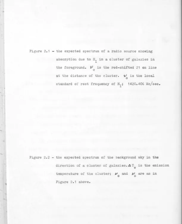
The expected spectrum of a radio source showing

absorption due to HI in a cluster of galaxies at a frequency,z{,

corresponding to the red-shift of the cluster is shown in

Figure 2.1. In principle, the absorption could be detected by

extremely accurate measurements of the antenna temperature of

the source over the range ~ to ~. Such a measurement, if

the absorption were as small as previous experiments have

suggested, present extreme calibration difficulties. The more

sensitive experiment used in this study was to detect, with a

frequency-switched receiver, the changes of spectral slope over

the frequency interval with respect to another "comparison"

radio source which would not be expected to show such changes.

Such a comparison source might be the moon, a galactic source

or an extra-galactic source with a red-shifted HI frequency

outside the range of t/

a to t/bo

With a frequency-switched receiver, when the

antenna is pointed at the "cold" sky (that is, no strong radio

the foreground. V is the red-shifted 21 cm line c

at the distance of the cluster. v is the local

o

standard of rest frequency of HI; 1420.406 Mc/sec.

Figure 2.2 - the expected spectrum of the background sky in the

direction of a cluster of galaxies.~Te is the emission

temperature of the cluster; '" c and J/_o are as in

11 c(

z

z

uJ

t-Z c( ~

ct

:>

~

~ UI

n.

~

w

t-~ Z Z uI I-2

c!

-I _{i I}

Vb

FREQUE.NCY ...

FI GURE

2

.1

I

SPEC.TRUM OF BACKGROUND SK~

S,",OWlNG CLUSTE.R EMISSION

I

,

~

I

~Te

I J l(

t/~ tJo

:

F'RE.QUE.NC'f ....

.

=

where g is the gain of the system in volts/ OK antenna

temperature

Tb is the antenna temperature of the background sky

and T is the receiver noise temperature.

n

The subscripts refer to the frequencies of the two receiver

channels.

With the antenna pointed at a radio source which is

much smaller than the beam and whose antenna temperature is T ,

a

,

the receiver output voltage,

eo

,

is given by;

eo'

=

g1(T +T + Tb ) - g (T + T + T ) a

1 n1 1 2 a2 n2 b2

Subtracting (2.1) from (2.2) gives the difference

in receiver output voltage, a, produced by alternately pOinting

the antenna at the source and at the adjacent sky;

=

(The assumption is made that the background sky temperatures

do not change between the on-source and off-source positions

of the antenna beam. )

Similarly, for a comparison source of antenna

temperature, T , the analagous on-source to off-source receiver

output deflection voltage, ~, is;

*

=

••.• (2.4)

From (2.3) and (2.4), ~T, the differential

temperature indicative of the spectral slope of the source

between the relevent frequencies is;

It can be seen from equation (2.5) that the measurement of

a comparison source eliminates the need of a precise knowledge

of the relative gains of the two receiver channels.

*

In the case where the Moon is used as a comparison source, since it is optically thick, equation (2.4) becomes;

=

g1(T - Tb ) - g2(T - Tb )

°1 1 c 2 2

In the frequency range, V to Vb' (T_b - Tb ) would be expected

a 2 1

to be constant and small and since g1 ~ g2 to a good approximation;

~

=

g T - g T + constant 1 c 2 c

1 2

Similarly, equation (2.5) and (2.6) have an additional term which

changes very slowly with frequency and in practice, is

The frequency interval from V to ~ is small so a b

that anywhere in that interval, to a first approximation,

T

IT

~ T

IT

and in practice, the gains of the two channels

a

1 c1 a c

are nearly equal so that g1"'" g2'" g.

constant over the frequency interval

The term (T - T ) is

c

2 c1

by definition so that

equation (2.5) becomes;

.6.T~ ~ R { Ta

g T

c

-

~}

+ constant

••••

(2.6a)

In the case where the moon is used as the comparison

source, as it is larger than the antenna beam and is a

blaok-body, and equation (2.6a) becomes;

i

{Ta _

£.}

g To ~

••••

(2

.

6b)

Since it is only desired to detect a change of 6 T

with frequency, it is clear that a precise value of T _a

IT

_c is

not really necessary although it can be easily determined.

Moreover, the significant quantity which changes with frequency,

a/~, is only a ratio of output deflections so that no precise

knowledge of the absolute gain of either receiver channel is

necessary.

A value of the receiver gain, g, can in principle be

obtained either from a measurement of T with respect to _c

receiver noise or from an injected noise calibration signal.

In these eXJeriments, the noise calibration signal was used

of the moon.

2.02 Experiment to Detect HI Emission from Clusters of Galaxies.

The spectrum of the background sky near the

centre of a cluster of galaxies might show emission from cluster

HI as in Figure 2.2.

The emission temperature,~T , may be detected by

e

alternately pointing the antenna at the cluster of galaxies and

at the adjacent sky when one channel is tuned to the cluster

frequency,

v ,

and the other channel is tuned to some other c

frequency outside the emission profile.

If channel 1 is tuned to

v

,

when the antenna is c

pointed at the cluster of galaxies, the receiver output

volta8e is;

=

T ) - g2 _{(T b} + T ) e 2 n₂

It is assumed that the cluster ~

-~ Tb

e

is optically thin so that

1

When the antenna is pOinted at the adjacent sky,

the oorresponding receiver output voltage is;

Subtracting (2.8) from (2.7) gives the difference in

y

=

g .6T

e

The assumption is again made that the background sky is uniform

over the region of the sky occupied by the cluster and the

adjacent region.

In principle, this experiment is extremely accurate and simple since apart from determining the gain, g, as in the previous section, precise values of the relative receiver gains and noise temperatures in the two channels are unnecessary.

However, because of the large angular extent of nearby clusters

of galaxies, the large angular separation between the on-cluster and off-cluster positions probably invalidates the assumption of background temperature uniformity used to derive equation (2.9)0

Moreover, the long intervals between observations due to

telescope driving time introduces additional uncertainties

because of long-term receiver instabilities. Consequently, in practice, it is difficult to measure ~T _e for nearby clusters to accuracies greater than a few hundredths of a degree.

2.03 General Intergalactic HI Emission Experiment.

)

V,

o

In principle, this step may be detected by absolute temperature measurements of the background sky over a range of frequencies

around

v.

This is essentially Goldstein's experiment in which

o

the accuracy depends largely on absolute clibrations over the frequency range. This major difficulty can be avoided by using the moon as a calibration source provided the antenna beam is smaller than the moon's disko

When the antenna is pOinted at the "COld" sky adjacent to the moon, the receiver output voltage is;

e

2 == g1 (T_b + T ) - g _{(T b} + T )

1 n₁ 2 2 n₂

••••

(2

.

10)

When the antenna is pointed at the moon, the receiver output voltage is;

••••

(2.11)

e

2/ == g 1 (T m+ T ) - g2 (T + T )

1 n1 m2 n2

where T is the antenna temperature of the moon. In both these

m

equations, contributions to the output due to the antenna response pattern outside the main beam are assumed equal and omittedo

Subtracting (2.10) from (2.11) gives the difference

of the receiver output, ~, when the antenna is alternately pointed at the moon and at the adjacent sky;

I

f3 ==

e

2 -

e

2

== g ₁ (T _m - Tb ) - g2 (T - Tb )

If a similar measurement is made on a galactic source which is small compared to the antenna beam, the corresponding deflection due to this source, ~,

=

Since the moon is a black-body larger than the beam, T

=

T

=

T and the differential temperature indicative of

m, m₂ m

the spectral slope of the background sky,LJT

b, is given from equations (2."2) and (2.13);

= T - T

b₂ b,

Tm - T b1

~

~. ~

[ T T g2 T -T

b a m , =

As Tb« T , and over the narrow

1

m,

frequency interval of observations, T --.JT , equation (2014) a, a

reduces to;

•••• (2.15)

Since it is only desired to detect a change of 6 Tb with frequency and provided the selected comparison source has no sharp spectral discontinuities, (T - T ) will not change with

a

2 a,

~requency, and no precise knowledge of T IT _{a; m} or (T _a - T ) are

2 a,

really necessary. (( T - T ) will of eourse change near

v

a

2 a, 0

frequencies were chosen to avoid fr'quencies near

v .)

o

The same considerations for determining g, apply

here as for the absorption experiment outlined in92.01.

The great advantage of this experiment as compared

to that of Goldstein is that, as in the absorption experiment, no precise absomute calibrations are necessaryo The change \nth

frequency in~Tb is given by a change with frequency in the

ratio of receiver output deflections due to the moon and to

2.1 The Antenna and Receiver

The antenna used was the 210-foot paraboloid

operated by the C.S.I.R.O. at the Australian National Radio

Astronomy Observatory near Parkes, N.S.W. At 21 cm, with the

particular feed used, the measured beam width was 13.8' and

to a good approximation over the central 25', the beam shape

was Gaussian.

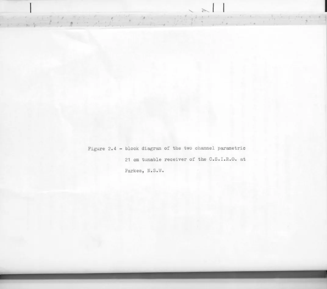
The receiver was developed and constructed by

B.J. Robinson and K.J. van Damme. A full description of the

receiver will be given by Robinson (in preparation). A

block diagram of the receiver shovdng the major components

and operating frequencies is shown in Figure 2.4. The total

system noise referred to the receiver input is about 190 oK.

The parametriC up-converter has a band width in

excess of 200 Mc/sec, a noise temperature of

~

70

oK and a

gain of nearly unity. The pump frequency of the up-converter

is switched at 400 c/sec to provide input frequency switching;

the stages following the up-converter are at constant frequency.

The second stage is a degenerate parametric amplifier with a band

width of ..., 6 Mc/sec, a noise temperature of ... 45 oK and a gain

of 20 db. The degenerate amplifier is followed by a conventional

crystal mixer, a pre-amplifier, an attenuator and an IF

amplifier. Several IF amplifiers with different band-widths

Figure 2.4 - block diagram of the two channel parametric 21 cm tunable receiver of the C.S.I.R.O. at

""c./~ CONVERT.

-

_~/s

'tao

Me/s

MULT

SWITCH ~

1

AMP.

""'-/l

+800 "c./~

MULT

10·'5 "'c./s

XTAL OSC.

4-00

rk..ls

2.J10 ~II

MUL T.

I

,---.,-400 "V

"8

r--1

J ..

·B ~c:/s c.(s OSC.

O'5C.

_osc

_.

FIGUR[

2.4-400

C./S

OET

PARAME.TRIC

H - LINE.

RE.CEIVE.R

AMP.

INTEGRATE

CHART

experiments 0 The band passes of these two IF amplifiers

nominally 1.5 Mc/sec and 500 kc/sec, are shown in Figures 2.5

and 2.6. The radio frequency detector is followed by a phase

-sensitive detector and a DC amplifier. The output is fed to

a chart recorder through a linear integrator.

The two switched frequencies for the up-converter

pump amplifier are generated by two highly stable Clapp

oscillators at 6.8 Mc/sec. The practical limit to the frequency

separation is determined partly by the band width of the pump

amplifier/multiPlier and partly by the size of switching

transients. For frequency separations less than 1 Mc/sec,

the switching transients are small and the relative gain

stability of the two channels of the receiver is good. As the

frequency separation is increased, the switching transients

become larger and the relative gain stability becomes poorer.

At the largest frequency separation used in practise, 5.5 Mc/sec,

the statistical errors of the output were about twice as large

as those for frequency separations less than 1 Mc/sec.

The gain of the degenerate amplifier is stabilized

by a servo-system which has been described by Robinson, Seeger,

van Damme and de Jager (1960). The degenerate amplifier is

thermally insulated and the extreme variations of temperature

from day to night were measured to be less than a few degrees C.

/

amplifier used in these experiments.

0

..D

a

z

-.(

C) -5

uJ

>

....

t!

..J W -\0

«

..D 0

o

z

-4

C) -5 W

>

-~

..J W -10

~

.'"\

/

.

•

_\

I •

\

/

•

_\

I

•

•

3

db. Bp..NDWIOTH = '))0 k,/!o

I

\

•

\

•

\

/

.

/

•

\

•

l.S.O z.~.O 30·0 }I.O

FR£QUE,NCY M~/a

F\GURE.

2.b

WlOE.

lor.

6ANOPASS

3

db. B,.,NDWIOTH •

I.'"

Mc/~

z.~ 0 }OO }IO

FR£QU(.NC'f Mel.

gain varied by less than a few per cento

The DC output stability depends on the total

stability of the phase-sensitive detector, DC amplifier and

integrator. For a constant input, the phase-sensitive detector

output varied by an amount corresponding to a few hundredths

of a degree K per day. The integrator output was accurate to an

amount corresponding to an antenna temperature of 0.01 oK

per integration. Over a typical period of observation of six

to ten hours, the combined errors of all these units was always

much less than the statistical error of the noise output.

In all measurements, the detector output was

maintained at a constant level by inserting attenuation in the

IF chain. Thus the values of antenna temperature due to the

various sources were related to each other through the

attenuations. This procedure eliminated effects of receiver

non-linearities and other factors considered later. The

attenuator consisted of a series of switched ~ sections and

the particular values of attenuation used for each source were

measured by comparison with a precision attenuator. It is

estimated that the values of attenuation obtained in this way

2.2 Sources of Error

2.21 Errors Due to the Antennao

Two possible sources of error arise from the

antenna; one due to pointing errors which might cause apparent

variations in source antenna temperature and the other due to

spillover and other zenith angle dependent effects.

The absolute pointing accuracy of the 210-foot

radio telescope is better than one minute of arc. At the

beginning of the observing periods, the apparent positions of

the relevant sources were checked and corrected for absolute

pointing errors. For those observations using the moon, the

moon's position was calculated in advance and these positions

were used. As the moon is considerably larger than the beam,

absolute pointing errors cause negligible variations in antenna

temperature. The relative resetability of the antenna during

any set of observations was probably better than 0.2'. As this

is a very small fraction of the 13.8' beam-width, errors due

to pointing may be disregarded.

The effects of spillover were estimated to be smallo

Errors due to this cause and to receiver variations arising from

flexure of the feed package should be dependent on zenith angle.

A search for such zenith angle effects was made in the data but

2.22 J~itations Caused by the Receiver.

The most fundamental limitation to the accuracy

of any measurement is caused by the random nature of the input noise signal and by the presence of receiver noise. In our

case, the total integration time was always sufficiently large

to make this limitation one of negligible importance.

The principle sources of error may be divided into two broad categories which, for the receiver used here at least,

may be considered separately, The first category contains all

effects which depend on the relative gains and noise temperatures

of the two channels and which may therefore be considered to

occur in the first frequency-switching sta8e of the receivero

In practise, errors in this first category were dominant.

In the second category are all other sources of

error caused by inaccuracies in the measurement of receiver

parameters in later stages of the receiver. Errors in this

category were generally of minor importance because of the

observing technique used.

a) First Category Errors.

Inequalities of the gain and noise temperature between

the two channels in the receiver produce an output even if the

antenna temperature at the two frequencies is equal. If the gain and noise temperature inequalities were stable with time,

their effect. Because these inequalities are not in general

stable, they produce errors.

If the time-varying changes in relative gain and

noise temperature are random and have periods shorter than the

integration times, their effect is indistinguishable from noise

and the receiver may be considered as having an effective noise temperature somewhat greater than the measured true input noise temperature. For the receiver used here, these short-term variations caused the effective receiver noise temperature to

be only slightly greater than the true noise temperature.

Because of the long total integration times used, this larger

contribution to the errors was usually negligible; typically,

it contributed""O.02 OK to the errors of a complete set of observations.

Much more important were the errors caused by

long-term variations in the relative gains and noise temperatures with periods longer than the individual integration periods. Long term changes of the relative noise temperature have little

effecto Long-term relative gain changes however produce values of the on-source to off-source deflection which vary

systematically with time. To some eitent, it was possible to

compensate for these long term changes since a relative gain

change produces, in general, a change in the off-source receiver

relation was determined between the size of the deflections and the off-source levels. This relations was then used to reduce all deflections to a common off-source level. However such a procedure can only reduce and not completely~iminate

this type of error. As the long-term relative gain stability decreased as the frequency separation increased, the magnitude

of these errors was a function of the frequency separation.

Typically, with a 3 Mc/sec frequency separation the errors

caused by long-term relative gain changes for a complete set of observations were,.., 0.05 oK.

b) Second Category Errors.

Gain modulation of the receiver at the switching

frequency produces a receiver output which varies with the

input signal strength. For the receiver used here, gain modulation produced a spurious output which was comparable to

the differential temperatures of the sources used. The gain modulation occurred wholly in the IF

amplifier due to assymetries in the waveform used to gate

switching transientso Because the attenuator preceeded the

IF amplifier, adding attenuation during the on-source measurement to keep the detector current level the same as for the off-source

measurement ensured that any output caused by gain modulation

would remain constant during both the on-source and off-source measurements. While this process eliminated errors due to gain

modulation and, as mentioned before, due to detector power

law non-linearities, it produces errors because of uncertainties

in the values of attenuations used. With an estimated accuracy

of less than 0.02 db in the attenuations, the resulting errors

were typically - 0.01 oK or less and hence negligible.

However, use of this method intriduced an additional error. Since attenuation was added when the antenna was

pointed at a radio source, both the deflection due to the

source and the receiver output base level due to noise

temperature and gain inequalities were attenuated. In order

to later reconstruct the on-source to off-source deflection,

it was necessary to determine the receiver output level when

the input to both receiver channels was known to be equal.

This basic "zero-level" output was obtained when the input

signal to the IF amplifier was generated by pre-amplifier noise alone. For any set of observations, the zero level was

o

known to~0.02 K. Errors due to uncertainty in this level were only of second-order importance except in the cases where

the source and the comparison sources did not have comparable

antenna temperatures. In these latter cases, with the wide

-band IF amplifier, the uncertainty in zero level typical~

contributed less than ~ 0001 OK to the final errors and hence

was negligible. The gain of the narrow-band IF amplifier

detector current from pre-amplifier noise to accurately determine the zero-level. For the narrow-band observations,

uncertainty in the zero level was estimated to contribute an

error of as much as ~O.05 OK which would appear systematically

in all the observations.

2023 Summary of Limitations.

For typical wide-band observations, the total

probable error of a measured differential temperature was - O.OS OK.

For the narrow band observations, the typical probable errors were approximately the same since the increased errors caused

by the use of the narrower bandwidth was offset by the improved

gain stability due to the smaller frequency separations used.

Comparison between wide and narrow band observations

indicated that systematic errors were present in the data due,

almost surely, to zero level uncertainties. It will be shown later that, as would be expected, the systematic errors in the wide band data were negligibly small compared to those in the

2.3 Method of Observations.

Observations were made only at night to eliminate

possible errors caused by the sun moving through the side-lobes

of the antenna pattern.

The basic observations consisted of recording the

receiver output while alternately pointing the antenna at

the source and at the adjacent off-source reference position.

These measurements were then repeated for the comparison source.

In order to reduce the effects of short-term variations in

receiver noise, the on-source and off-source outputs were

integrated for 100 seconds and recorded. In order to reduce

the effects of long-term variations, such a sequence of observations

was made for only about an hour alternately with a similar

sequence for the comparison source. This period was a compromise

between a shorter period which would entail a greater loss of

observing time driving the telescope between the two sources

and a longer time which would result in poorer compensation

for changes in receiver parameters.

All observations of sources for which the moon was

used as the comparison source were conducted on the few nights

each month that the moon and the source were within the

telescope sky coverage at the same timeo Particularly for

Virgo A, which is near the northern limit of the telescope

and measurements were only made on one frequency pair per nighto

Before observations began, the receiver was carefully

tuned to minimize the gain inequality between the two channelso

The noise lamp calibration signal was measured before and after

the observations. The basic receiver zero level for the night

was measured before and after the observations as well as

during the periods that the telescope was being driven between

the source and the comparison source. The attenuations used

during the night were recorded and later measured by comparison

2.4 Calibration

The primary calibration used in these experiments

was supplied by a switched noise lamp. Prior to November, 1963,

the ratio of the noise lamp temperatures to the antenna

temperature of 3C353 was measured to be 0.420. In the course

of absorption observations of 3C353, the ratio of the antenna

temperature of 3C353 to that of the moon was determined to be

+

0.2355 -0.0014. If the antenna efficiency were 1.0, the antenna

temperature of the moon would be identical to the brightness

temperature of the moon, 230 oK, and the noise lamp temperature

would be 22.7 oK.

The effective temperature of the noise lamp was

defined to be this value. The effective antenna temperature

of any radio source derived by using this value is then the true antenna temperature divided by the true antenna efficiency.

In this way, no implicit assumptions were made of the absolute

antenna efficiency and for sources uniform over the antenna

beam, the effective antenna temperature is equivalent to the

brightness temperature of the source.

In November 1963, the reflector plate behind the

dipole at the feed package was modified resulting in a slightly

higher antenna efficiency than earlier. The new ratiO of the

noise lamp temperature to the antenna temperature of 3C353 was

o

OHAPrER THREEo T$ OBSERVATIONS.

3.00 General

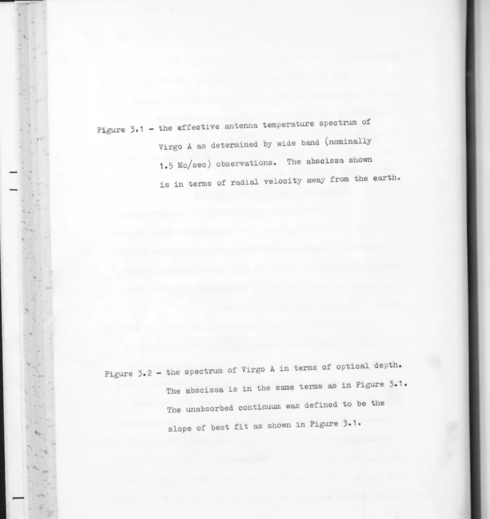
3.01 Antenna Temperatures and Spectral Slopes of Radio Sources In the absence of absorption, the differential

temperatures determined for any radio source can be used to

determine the slope of the source's antenna temperature spectrum.

This slope is not necessarily equivalent to the standard flux spectral index, except for those sources with dimensions much smaller than the antenna beam. For a uniform source, much larger than the beam, the antenna temperature spectral slope is equivalent to the brightness temperature spectral slope and for partially resolved sources, the antenna temperature spectral slope is intermediate between the flux and brightness temperature spectral slope.

For the seven sources used in the course of these

experiments, 30273 and 30353 are essentially unresolved at 21 cm,

the moon is uniform over the antenna beam and Virgo A, M 17, Pic tor A and Fornax A are partially resolved. The expected antenna temperature spectral slopes, in the absence of absorption, for the four latter sources were calculated by

computer from published brightness distributions of the sources.

•

this study.

SOURCE

Moon

Virgo A Core Virgo A Halo 3C273

3C353 Fornax A

Pictor A

11117

Ili17

M

17

FLUX SPECTRAL

INDEX

+2.0 -0.44 1 -1.02 1

-0.23 3

-0.64 4 -0.7 1 -0.7 1

05

05

05

rotes to TABLE 3.1

ASSUMED

MODEL

Uniform over beam 2 Point source

Gaussian 6.5' dia2

Point source

Point source

Price6profile Broten7profile LittleSprofile

Labrum et al9prOfile Labrum without eas

t-ern Extension

1. Kellerman, K.I., Ap.J., 140, 969, 1964.

CALCULATED

ANT. TEIJiP.

SWPE

0.0

-0044} 10 -1.52 -0.92 -0.23

-0064

_2.0011

_0.S311

-0.56 -0.40 -0.30

2. .1altby, P. and r1offet, A.T., Obs.Cal-Tech. ,

.1,

1964.

3. Yellerman, K.I., private communication.

4. Conway, R.G., Kellerm::n, 1':.1. and Long, R.J., LoN .R.A.S. , 125,

261, 10_63.

5. If optically thin - see Aopendix B.

6. Price, ! ., private communication, about 10' in diameter.

7. Broten, N., private communication.

S. Little, A., Ap.J.,

121,

164, 1963.

9. Labrum, I-T.R., Krishnan, J., Pay ten, ','I.J., and Harting, E.,

Gaussian with a half-power width of 13.81

• The products of

the antenna gain and the source intensities over the beam were integrated numerically at two adjacent frequencies at

2

21 cm assuming that the antenna gain varied as V and that the

beam-width decreased as 1/V 0 For simplicity, it was assumed

that the source profiles used were representative of the source

in all directions and the integration was only carried out

in one direction.

The calculated antenna temperature spectral slopes

based on published flux spectral indices and models of brightness

distributions are shown in Table 3.1.

3.02 The Moon

The moon has a mean diameter of 31 1 which covers more than

99%

of the total main antenna beam solid angle.

Because the coverage is so complete, a change in frequency near 21 cm produces a negligible change in antenna temperature

assuming the moon is a black body.

The brightness temperature of the moon has been

measured at many frequencies and the evidence indicates that

the moon's spectrum is characteristic of a black body. The

o

brightness temperature of the moon was assumed to be 230 K.

This value is the approximate mean of a number of published

The accuracy of this estimate is probably 5%. All the results

in this study were referred to this assumed brightness temperature

so that, not withstanding any absolute error, all the data would

be internally consistent.

It was assumed that the brightness temperature of the

moon did not change with phase. In any case all the relevent

observations took place near full moon so that this approximation

results in a negligible error at 21 em.

3.03 Data Analysis

The data was processed by computer. The

recorded deflections were first corrected for the relevant

attenuations to give a and ~ as defined in

9

2.01 and

9

2•03. Then the alternate sets of source and comparison source

deflections were averaged to produce

a

and ~ and the sum of the standard deviations, ~ , was determined.

o

To reduce the effect of long-term gain variations,

the data was investigated to detect a possible correlation

between the on-source to off-source deflections, a, and the

off-source output level ~. This was done by first determining

a least-square solution to the linear equation;

a

=

a + a,

<I

o

The constant a. is a measure of the rate of change of a with/ ·

equation relating ~ andJ25;

=

where

b

==

To

1 - Ta • a₁

Using the equations (3.2) and (3.3) all the data of the sets of ~IS were used to determine b ₀. _'

The sum of the standard deviations of a_o and b 0' <J

1, was a measure of how precisely the data conformed to equations (3.1) to (3.4). If <J

1

<

~o' it was considered that the correlations

between ex and ¢ and ~ and

¢

were significant and due to a systematic relative gain change so that a _o andb were used in

o

place of

a

and ~ to determine the final differential temperature.

If

0;

~~, it was considered that detectable long-term relative gain variations were not present and

a

and ~ were used to

determine the differential temperatureo

Zenith angle dependence in the data was checked in a similar fashion but no significant correlation was ever

detected.

(except in the case of the Fornax A observations*). The

scatter in the individual determinations suggest that the

average value used was correct to -- 1%. This accuracy is

more than sufficient since TaiTe or TalTm do not need to be

known to any great precision.

The computer output for any complete set of data

I

was a differential temperature, 6 T , where;

=

~

{ Ta _

~

}

g Tc ~

For the absorption experiments outlined in ~ 2.01,

this differential temperature is related to the differential

temperature of the source (from equation (2.6a)), ~T, by;

=

AT' Ta

u. + Tc

and in the more common case where the moon was used as the

comparison source, from equation (2.6b);

*

Fornax

A

is highly polarized. Because it and its comparison source, Pictor A, was observed over a range of position angles,

the value of TaiTe determined for any set of observations was

... y . ,

the differential temperature of the background sky, ~Tb' is

(

related to 6. T by;

- (T - T

;L

a2

a1

'f

•••• (3.8)

The quantities, ~T' , will be shown in the data

tables for each experiment along with an associated statistical

probable error and weight.

The probable error of any differential temperature

was defined to be;

P.E. =

g

rn

where

cr-

=

Il: or a- whichever was relevent.

1 0

n

=

number of determinations of a and ~ made

and g

=

receiver gain.

This probable error will be referred to as the statistical

probable erroro

Since instability of the relative gain of the two

channels was the principle source of error, the data was

weighted according to the inequality of gain in the two channels

as well as by the size of the probable errors. Since the

size of ~ was a measure of the gain inequality the weight of

any differential temperature was defined to be;

W

=

(100 -

@)

103 (P.E. )2