White Rose Research Online URL for this paper:
http://eprints.whiterose.ac.uk/135937/
Version: Accepted Version
Article:
Aldridge, M orcid.org/0000-0002-9347-1586 (2019) Individual testing is optimal for
nonadaptive group testing in the linear regime. IEEE Transactions on Information Theory,
65 (4). pp. 2058-2061. ISSN 0018-9448
https://doi.org/10.1109/TIT.2018.2873136
© 2018 IEEE. This is an author produced version of a paper accepted for publication in
IEEE Transactions on Information Theory. Uploaded in accordance with the publisher's
self-archiving policy. Personal use of this material is permitted. Permission from IEEE must
be obtained for all other users, including reprinting/ republishing this material for
advertising or promotional purposes, creating new collective works for resale or
redistribution to servers or lists, or reuse of any copyrighted components of this work in
other works.
[email protected] https://eprints.whiterose.ac.uk/
Reuse
Items deposited in White Rose Research Online are protected by copyright, with all rights reserved unless indicated otherwise. They may be downloaded and/or printed for private study, or other acts as permitted by national copyright laws. The publisher or other rights holders may allow further reproduction and re-use of the full text version. This is indicated by the licence information on the White Rose Research Online record for the item.
Takedown
If you consider content in White Rose Research Online to be in breach of UK law, please notify us by
Individual Testing is Optimal for Nonadaptive
Group Testing in the Linear Regime
Matthew Aldridge
Abstract—We consider nonadaptive probabilistic group testing
in the linear regime, where each ofnitems is defective indepen-dently with probabilityp∈ (0,1), andpis a constant independent ofn. We show that testing each item individually is optimal, in the sense that with fewer than n tests the error probability is bounded away from zero.
I. INTRODUCTION
Group testing considers the following problem: Given n items of which some are ‘defective’, how many ‘pooled tests’ are required to accurately recover the defective set? Each pooled test is performed on a subset of items: the test is negative if all items in the test are nondefective, and is positive if at least one item in the test is defective.
In Dorfman’s original work [1], the application was to test men enlisting into the U.S. army for syphilis using a blood test. Dorfman noted that one could test pools of mixed blood samples and use fewer tests than testing each blood sample individually. The test result from such a pool should be negative if every blood sample in the pool is free of the disease, while the test result should be positive if at least one of the blood samples is contaminated. Other applications of group testing include in biology [2], signal processing [3], and communications [4], to name just a few.
The most important distinction between types of group testing is between:
• Nonadaptive testing, where all the tests are designed in
advance.
• Adaptive testing, where the items placed in a test can
depend on the results of previous tests.
This paper considers nonadaptive testing. Nonadaptive testing is important for modern applications of group testing, where an experimenter wishes to perform a large number of expensive or time-consuming tests which are required to be performed in parallel.
A second important consideration is how many defective items there are. In this paper, we consider thelinear regime, where the number of defective itemskis a constant proportion p ∈ (0,1) of the n items. A lot of group testing work has concerned the very sparse regime where k is constant as n → ∞ [5]–[7] or the sparse regime k = Θ(nα) as
n→ ∞for some α <1 [8]–[12]. However, we argue that the linear regime is more appropriate for many applications. For example, in Dorfman’s original set-up, we might expect each person joining the army to have a similar prior probability p
The author is with the School of Mathematics, University of Leeds, Leeds, U.K. E-mail: [email protected].
of having the disease, and that this probability should remain roughly constant as more people join, rather than tending towards 0; thus one expects k ≈ pn to grow linearly with n.
Within nonadaptive group testing in the linear regime, two cases have received most consideration in the literature:
• Combinatorial zero-error testing:The defective set is any
subset of{1,2, . . . ,n} with given sizek, and one wishes to find the defective set with certainty, whichever such set it is. One assumes that k/n tends to a constantp∈ (0,1)
as n→ ∞. [13]–[16]
• Probabilistic small-error testing: We assume each item
is defective with probability p, independent of all other items, where p ∈ (0,1) stays fixed. We want to find the defective set with arbitrarily small error probability (averaged over the random defective set). [16]–[20] This paper considers probabilistic small-error testing. One could consider the case of combinatorial small-error testing, where exactly k ∼ pn items are defective chosen uniformly at random, together with a small-error criterion. However, we claim that the probabilistic model of independent defectivity is more realistic in applications: again, soldiers might each have a disease with some known prevalence p, but it is un-realistic to knowexactlyhow many soldiers have the disease. The choice between combinatorial (known k) or probabilistic (independentp) set-ups tends not to substantially affect results, as the probabilistic case sees concentration of the number defectives around k = pn; we briefly discuss in Section IV that our result may extend to the combinatorial small-error case. Probabilistic zero-error testing is not of interest: since any of the2T subsets of items could be the defective set, it is immediate that individual testing is optimal.
We emphasise that we are looking for full reconstruction; that is, we only succeed if we find the exact defective set, classifying every defective and nondefective item correctly. (See Definition 2 for formal definitions.)
For group testing in the linear regime, it is easy to see that the optimal scaling is the number of tests T scaling linearly withn. A simple counting bound (see, for example, [8], [11], [20]) shows that we requireT ≥ (1−δ)H(p)nfor large enough n, where H(p)is the binary entropy. Meanwhile, testing each item individually requires T = n tests, and succeeds with
certainty. (In the combinatorial case, T = n−1 suffices, as
the status of the final item can be inferred from whether k or k−1 defective items have been already discovered from individual tests.) Thus we are interested in the question: when is individual testing withT =n (orn−1) optimal, and when
In the adaptive combinatorial zero-error case it is known that individual testing is optimal forp≥1−log32≈0.369[14] and suboptimal for p <1/3 [13], [21] for all n. Hu, Hwang and Wang [13] conjecture thatp=1/3is the correct threshold. In forthcoming work, Aldridge [16] gives algorithms using T <1.11H(p)n tests for all p≤1/2 and large n.
In theadaptive probabilistic small-error case, it is known that individual testing is optimal for p≥ (3−√5)/2≈0.382
and suboptimal for p < (3 −√5)/2 [17] for n sufficiently large. In forthcoming work, Aldridge [16] gives algorithms usingT <1.05H(p)n tests for all p ≤1/2 and largen.
In thenonadaptive combinatorial zero-errorcase, it is well known that individual testing is optimal when k grows faster than roughly √n, which is the case for all p ∈ (0,1) in the linear regime forn sufficiently large [5], [15], [22], [23].
This leaves the nonadaptive probabilistic small-errorcase. In this paper, we show that individual testing is optimal for all p∈ (0,1)and alln.
Theorem 1:Consider probabilistic nonadaptive group testing
where each ofnitems is independently defective with a given probabilityp∈ (0,1), independent ofn. Suppose we useT <n tests. Then there exists a constant ǫ =ǫ(p)>0, independent of n, such that the average error probability is at leastǫ.
(The average error probability is defined formally in Defi-nition 2.)
The previous best result was by Agarwal, Jaggi and Mazum-dar [20]. They used a simple entropy argument to show that individual testing is optimal for p≥ (3−√5)/2≈0.382, and a more complicated argument using Madiman–Tetali inequali-ties to extend this top>0.347. We extend this to allp∈ (0,1). Further, Agarwalet al.use a weaker definition of ‘optimality’ than we do here: they show that the error probability is bounded away from 0 as n → ∞ when T < (1−δ)n for some δ > 0, whereas we show that the error probability is bounded away from0 for anyT <n.
Wadayama [19] had claimed to be able to beat individual testing for somepin work that was later retracted in part [24]. We discuss this matter further in Section IV.
Finally, we note that other scaling regimes than the linear regime have been studied, notably the sparse regimek=Θ(nα)
for different values of the sparsity parameter α ∈ [0,1). In these regimes, forn sufficiently large: adaptive testing always outperforms individual testing [8], [15], [25], nonadaptive small-error testing always outperforms individual testing [7], [9], [10], [12], [26], and nonadaptive zero-error testing out-performs individual testing for α <1/2 but not for α > 1/2
[5], [22], [23], [27].
II. DEFINITIONS AND NOTATION
We fix some notation and state some important definitions.
Definition 2: There are n items, and we perform T tests.
A nonadaptive test design can be defined by a test matrix
X=(xti) ∈ {0,1}T×n, where xti =1 means itemi is in testt,
and xti=0 means it is not.
Given a test designXand a defective setK ⊆ {1,2, . . . ,n}, the outcomesy=(yt) ∈ {0,1}T are given by yt =0 if xti=0
for alli ∈ K, and yt =1 otherwise.
An estimate of the defective set is a (possibly random) functionKˆ =K(Xˆ ,y) ⊆ {1,2, . . . ,n}.
The average error probabilityis
P(error)= Õ K ⊆ {1,2,...,n}
p|K |(1−p)n−|K |P K(Xˆ ,y),K,
where y is related toX andK as above, and the probability
P can be replaced by an indicator function if the estimate Kˆ
is nonrandom.
The concept of an item being ‘disguised’ will be important later.
Definition 3: Fix a test design X and a defective set K.
Given an item i (either defective or nondefective) contained in a test t, we say that itemi isdisguised in testt if at least one of the other items in that test is defective; that is, if there exists a j ∈ K,j ,i, withxt j=1. We say that itemiistotally
disguised if it is disguised in every test it is contained in.
Lemma 4: Consider probabilistic group testing with
defec-tive probabilityp. Fix a test designX, and writewt=Íni=1xti for theweight of testt; that is, the number of items in testt. Further, write Di for the event that itemi is totally disguised.
Then
P(Di) ≥
Ö
t:xt i=1
(1−qwt−1 ),
whereq=1−p.
This is essentially Lemma 4 of [20]; we give a shorter proof here based on the FKG inequality (see for example [28], [29, Section 2.2]).
Proof: For a test t containing item i, write Dt,i for the
event that i is disguised int. Clearly we have
P(Di)=P
Ù
t:xt i=1
Dt,i
!
.
Further, for a test t containing item i we have P(Dt,i) =1− qwt−1
, sincei is disguised in t unless the other wt−1 items
in the test are all nondefective. Note also that the Dt,i are
increasing events, in the sense that for L ⊆ K the indicator
functions satisfy 1Dt,i(L) ≤ 1Dt,i(K). The FKG inequality
tells us that increasing events are positively associated, in that
P Ù
t:xt i=1
Dt,i
! ≥ Ö
t:xt i=1
P(Dt,i),
and the result follows.
III. PROOF OF MAIN THEOREM
We are ready to proceed with the proof of Theorem 1.
Proof of Theorem 1: The key idea is the following:
Fixn. Fix a test designXwithT <n tests. Without loss of generality we may assume there are no tests of weightswt=0
or1. All weight-0 ‘empty’ tests can be removed. If there is a weight-1test, we can remove it and the item it tests, repeating until there are no weight-1 tests remaining. These removals leave p the same, do not increase the error probability, and reduceT/n, since we hadT/n<1 to start with.
From Lemma 4, the probability that item i is totally dis-guised is bounded by
P(Di) ≥
Ö
t:xt i=1
(1−qwt−1 ),
WriteL(i)for the natural logarithm of this bound, soP(Di) ≥
eL(i), where
L(i)=log
Ö
t:xt i=1
(1−qwt−1 )
=
Õ
t:xt i=1
log(1−qwt−1 )
= T
Õ
t=1
xtilog(1−qwt−1).
We must show that, for somei, L(i) is bounded from below, independent ofn. Then with probability at least eL(i)we have a totally disguised item, and the theorem follows.
Write L¯ for the mean value of L(i), averaged over all i items. (Note that L¯ is negative.) Then we have
¯
L =1
n
n
Õ
i=1
L(i)
=1
n
n
Õ
i=1
T
Õ
t=1
xtilog(1−qwt−1)
= 1
n
T
Õ
t=1
n
Õ
i=1
xti
!
log(1−qwt−1 )
= 1
n
T
Õ
t=1
wtlog(1−qwt−1)
≥Tn min
t=1,2,...,T
wtlog(1−qwt−1) (1)
≥ min
t=1,2,...,T
wtlog(1−qwt−1) (2)
≥ min
w=2,3,...
wlog(1−qw−1) =:L∗. (3)
Going from (1) to (2) we have used the assumptionT/n ≤1
(and that T/n is multiplied by a negative expression), and going from (2) to (3) we used assumption that no test has weight 0 or 1. Note further that the the bound L∗ is indeed finite, since, for q <1, the function w 7→wlog(1−qw−1) is
continuous for w∈ [2,∞), finite at w=2, and tends to 0 as w→ ∞.
Since L¯ is the mean of the L(i)s, there is certainly somei with L(i) ≥ L¯ ≥ L∗, and thus some i withP(Di) ≥ eL∗. We are done.
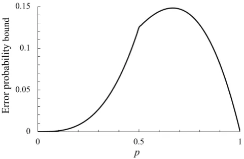
Inspecting the proof, we see immediately that, whenT <n, we have an explicit bound on the error probability of
P(error) ≥ǫ(p)=min{p,q}eL ∗
[image:4.595.310.551.55.212.2], (4)
Fig. 1. The error probability bound (4), plotted against the prevalencep.
with L∗ as in (3). The bound (4) is plotted in Figure 1. It is simple to compute the bound for any p. In particular, one can easily check that forp>0.161the minimum in (3) is achieved atw=2, giving L∗=2 log(1−q1)=2 logp, giving eL∗
=p2 and therefore the very simple bound
P(error) ≥
(
qp2 p ≥1/2,
p3 0.161<p<1/2.
On the other hand, we can consider the limit asp→0. By comparing L∗ to the expressionwlog(1−qw), which can be
explicitly minimised using calculus, we see that the optimal
win (3) is asymptotically
w∼ −log 2 logq ∼
log 2
p as p→0,
giving L∗ ∼ −(log 2)2/p, and the asymptotic expression for
ǫ(p)in (4) as
ǫ(p) ∼pexp
−(log 2) 2
p
≈pexp
−0.480p
as p→0.
By being more careful at the step from (1) to (2), we see that whenT <(1−δ)nwe can improve the bound (4) to
P(error) ≥min{p,q}e(1−δ)L∗.
Note that in the proof we only bounded the probability that one particular item is wrongly decoded, so the bound (4), while explicit, simple to compute, and bounded away from 0, is unlikely to be tight for many cases.
IV. CLOSING REMARKS
We have shown that individual testing is optimal for small-error nonadaptive testing in the linear regime for all p∈ (0,1). Our result here contradicts a result of Wadayama [19, Theorem 2], later retracted [24], which claimed arbitrarily low error probabilities for n sufficiently large withT/n <1. Wadayama useddoubly regulartest designs chosen at random subject to each item being inltests and each test containingr items, wherelandrare kept fixed asn→ ∞. Sincel/r=T/n,
bounded below byP(Di) ≥ (1−q − ), a constant greater than
0 for r > l ≥ 1. Thus these designs cannot have arbitrarily low error probability.
A note of caution with our result is due. We have only shown that the error probability cannot be made arbitrarily small – however, it might be very small. For example, we see from Figure 1 that the error bound given by (4) is very small for p < 0.1. Thus, for some given nonzero error tolerances, and some p and n, it may still be that random designs can be profitably used in applications – suggestions include Bernoulli random designs [6], [7], [9], [10], [18], [26], designs with constant tests-per-item [12], [18], or Wadayama’s doubly regular designs [18], [19]. Further ‘finite blocklength’ analysis of these designs would be useful in investigating this point.
It seems likely that a similar result to Theorem 1 holds for small-error testing under the combinatorial model, where exactly k ∼ pn items are defective, chosen uniformly at random. We conjecture that for T < n −1 (recalling again that the final item’s status can be inferred from the status of the other items) the error probability is bounded away from
0. The main difficulty here is that the FKG inequality used in the proof of Lemma 4 is reliant on the independence of the defectivity of items. Further, one would have to be careful in asserting that the existence of a totally disguised item ensures a probability of error bounded away from0. One work-around to the latter point might be to show there is likely to be both a totally disguised defective item and a totally disguised nondefective item, so the tester cannot know which is which. We have shown that, with a small-error criterion, individual testing is optimal in the linear regime k ∼ pn for p > 0, while it is known that individual testing is suboptimal when
k=Θ(nα
)for anyα <1 [7], [9], [10], [26]. This leaves open exactly when individual testing becomes suboptimal. For ex-ample, is individual testing optimal or not when k∼n/logn? The method employed here required p to be bounded away from 0; with p = 1/logn, for example, a totally disguised
item could be safely assumed to be nondefective with error probability tending to0.
ACKNOWLEDGEMENTS
The author thanks Sidharth Jaggi, Jonathan Scarlett and anonymous reviewers for useful comments. This research was conducted in part while the author was supported by the Heilbronn Institute for Mathematical Research.
REFERENCES
[1] R. Dorfman, “The detection of defective members of large populations,”
Ann. Math. Statist., vol. 14, no. 4, pp. 436–440, 12 1943.
[2] S. D. Walter, S. W. Hildreth, and B. J. Beaty, “Estimation of infection rates in populations of organisms using pools of variable size,”American
Journal of Epidemiology, vol. 112, no. 1, pp. 124–128, 1980.
[3] A. C. Gilbert, M. A. Iwen, and M. J. Strauss, “Group testing and sparse signal recovery,” in2008 42nd Asilomar Conference on Signals, Systems
and Computers, 2008, pp. 1059–1063.
[4] M. K. Varanasi, “Group detection for synchronous Gaussian code-division multiple-access channels,” IEEE Transactions on Information
Theory, vol. 41, no. 4, pp. 1083–1096, 1995.
[5] A. G. D’yachkov and V. V. Rykov, “Bounds on the length of disjunctive codes,”Problemy Peredachi Informatsii, vol. 18, no. 3, pp. 7–13, 1982, translation:Problems of Information Transmission, vol. 18, no. 3, pp. 166–171, 1982.
[6] M. Malyutov, “Search for sparse active inputs: a review,” inInformation Theory, Combinatorics, and Search Theory: In Memory of Rudolf
Ahlswede, H. Aydinian, F. Cicalese, and C. Deppe, Eds. Springer,
2013, pp. 609–647.
[7] G. K. Atia and V. Saligrama, “Boolean compressed sensing and noisy group testing,”IEEE Transactions on Information Theory, vol. 58, no. 3, pp. 1880–1901, 2012.
[8] L. Baldassini, O. Johnson, and M. Aldridge, “The capacity of adaptive group testing,” in2013 IEEE International Symposium on Information
Theory Proceedings (ISIT), 2013, pp. 2676–2680.
[9] M. Aldridge, L. Baldassini, and O. Johnson, “Group testing algorithms: bounds and simulations,” IEEE Transactions on Information Theory, vol. 60, no. 6, pp. 3671–3687, 2014.
[10] J. Scarlett and V. Cevher, “Limits on support recovery with probabilistic models: an information-theoretic framework,” IEEE Transactions on
Information Theory, vol. 63, no. 1, pp. 593–620, 2017.
[11] T. Kealy, O. Johnson, and R. Piechocki, “The capacity of non-identical adaptive group testing,” in52nd Annual Allerton Conference on
Com-munication, Control, and Computing, 2014, pp. 101–108.
[12] O. Johnson, M. Aldridge, and J. Scarlett, “Performance of group testing algorithms with near-constant tests-per-item,” IEEE Transactions on
Information Theory, 2018.
[13] M. C. Hu, F. K. Hwang, and J. K. Wang, “A boundary problem for group testing,”SIAM Journal on Algebraic Discrete Methods, vol. 2, no. 2, pp. 81–87, 1981.
[14] L. Riccio and C. J. Colbourn, “Sharper bounds in adaptive group testing,”Taiwanese Journal of Mathematics, vol. 4, no. 4, pp. 669–673, 2000.
[15] S. H. Huang and F. K. Hwang, “When is individual testing optimal for nonadaptive group testing?”SIAM Journal on Discrete Mathematics, vol. 14, no. 4, pp. 540–548, 2001.
[16] M. Aldridge, “Rates for adaptive group testing in the linear regime,” 2018, in preparation.
[17] P. Ungar, “The cutoff point for group testing,”Communications on Pure
and Applied Mathematics, vol. 13, no. 1, pp. 49–54, 1960.
[18] M. M´ezard, M. Tarzia, and C. Toninelli, “Group testing with random pools: Phase transitions and optimal strategy,” Journal of Statistical
Physics, vol. 131, no. 5, pp. 783–801, 2008.
[19] T. Wadayama, “Nonadaptive group testing based on sparse pooling graphs,”IEEE Transactions on Information Theory, vol. 63, no. 3, pp. 1525–1534, 2017, see also [24].
[20] A. Agarwal, S. Jaggi, and A. Mazumdar, “Novel impossibility results for group-testing,” 2018, arXiv:1801.02701 [cs.IT].
[21] P. Fischer, N. Klasner, and I. Wegenera, “On the cut-off point for combinatorial group testing,” Discrete Applied Mathematics, vol. 91, no. 1, pp. 83–92, 1999.
[22] H.-B. Chen and F. K. Hwang, “Exploring the missing link among
d-separable, d¯-separable and d-disjunct matrices,” Discrete Applied
Mathematics, vol. 155, no. 5, pp. 662–664, 2007.
[23] D. Du and F. Hwang,Combinatorial Group Testing and Its Applications, 2nd ed. World Scientific, 1999.
[24] T. Wadayama, “Comments on “Nonadaptive group testing based on sparse pooling graphs”,” IEEE Transactions on Information Theory, vol. 64, no. 6, pp. 4686–4686, June 2018.
[25] F. K. Hwang, “A method for detecting all defective members in a popu-lation by group testing,”Journal of the American Statistical Association, vol. 67, no. 339, pp. 605–608, 1972.
[26] C. L. Chan, P. H. Che, S. Jaggi, and V. Saligrama, “Non-adaptive prob-abilistic group testing with noisy measurements: near-optimal bounds with efficient algorithms,” in 49th Annual Allerton Conference on
Communication, Control, and Computing, 2011, pp. 1832–1839.
[27] W. H. Kautz and R. C. Singleton, “Nonrandom binary superimposed codes,”IEEE Transactions on Information Theory, vol. 10, no. 4, pp. 363–377, 1964.
[28] C. M. Fortuin, P. W. Kasteleyn, and J. Ginibre, “Correlation inequalities on some partially ordered sets,” Communications in Mathematical
Physics, vol. 22, no. 2, pp. 89–103, 1971.