Counting linear extensions: Parameterizations by treewidth

White Rose Research Online URL for this paper:

http://eprints.whiterose.ac.uk/146315/

Version: Published Version

Article:

Eiben, E. orcid.org/0000-0003-2628-3435, Ganian, R., Kangas, K. et al. (1 more author)

(2019) Counting linear extensions: Parameterizations by treewidth. Algorithmica, 81 (4).

pp. 1657-1683. ISSN 0178-4617

https://doi.org/10.1007/s00453-018-0496-4

[email protected] https://eprints.whiterose.ac.uk/ Reuse

This article is distributed under the terms of the Creative Commons Attribution (CC BY) licence. This licence allows you to distribute, remix, tweak, and build upon the work, even commercially, as long as you credit the authors for the original work. More information and the full terms of the licence here:

https://creativecommons.org/licenses/

Takedown

If you consider content in White Rose Research Online to be in breach of UK law, please notify us by

https://doi.org/10.1007/s00453-018-0496-4

Counting Linear Extensions: Parameterizations

by Treewidth

E. Eiben1 ·R. Ganian2·K. Kangas3·S. Ordyniak4

Received: 16 November 2016 / Accepted: 3 August 2018 / Published online: 4 September 2018 © The Author(s) 2018

Abstract

We consider the #P-complete problem of counting the number of linear extensions of a poset(#LE); a fundamental problem in order theory with applications in a variety of distinct areas. In particular, we study the complexity of#LEparameterized by the well-known decompositional parameter treewidth for two natural graphical representations of the input poset, i.e., the cover and the incomparability graph. Our main result shows that#LEis fixed-parameter intractable parameterized by the treewidth of the cover graph. This resolves an open problem recently posed in the Dagstuhl seminar on Exact Algorithms. On the positive side we show that#LEbecomes fixed-parameter tractable parameterized by the treewidth of the incomparability graph.

Keywords Partially ordered sets·Linear extensions·Parameterized complexity· Structural parameters·Treewidth

1 Introduction

Counting the number of linear extensions of a poset is a fundamental problem of order theory that has applications in a variety of distinct areas such as sorting [30], sequence analysis [25], convex rank tests [27], sampling schemes of Bayesian networks [28], and preference reasoning [24]. Determining the exact number of linear extensions of a given poset is known to be #P-complete [6] already for posets of height at least 3. Informally, #P-complete problems are as hard as counting the number of accept-ing paths of any nondeterministic Turaccept-ing machine, implyaccept-ing that such problems are not tractable unlessP=NP. The currently fastest known method for counting linear

B

[email protected]

1 _{Department of Informatics, University of Bergen, Bergen, Norway} 2 _{Algorithms and Complexity Group, TU Wien, Vienna, Austria}

extensions of a generaln-element poset is by dynamic programming over the lattice of downsets and runs in timeO(2n_{·n)[10]. Polynomial time algorithms have been found}

for various special cases such as series-parallel posets [26] and posets whose cover graph is a (poly)tree [2]. Fully polynomial time randomized approximation schemes are known for estimating the number of linear extensions [7,13].

Due to the inherent difficulty of the problem, it is natural to study whether it can be solved efficiently by exploiting the structure of the input poset. In this respect, the parameterized complexity framework [9,12] allows a refined view of the interactions between various forms of structure in the input and the running time of algorithms. The idea of the framework is to measure the complexity of problems not only in terms of input sizes, but also with respect to an additional numerical parameter. The goal is then to develop so-calledfpt algorithms, which are algorithms that run in time f(k)nO(1)wherenis the input size and f is a computable function depending only on the parameterk. A less favorable outcome is a so-calledXPalgorithm, which runs in timenf(k); the existence of such algorithms then gives rise to the respective complexity classesFPT(fixed-parameter tractable) andXP.

The first steps in this general direction have been taken, e.g., in [19], using the decomposition diameter as a parameter, in [15] using a parameter called activity for N-free posets, and very recently in [22], where the treewidth of the so-called cover graph was considered as a parameter. Also the exact dynamic programming algorithm [10] can be shown to run in timeO(nw·w)for a poset withnelements and widthw(the size of the largest anti-chain). Interestingly, none of these efforts has so far led to an fpt algorithm.

We believe that this uncertainty about the exact complexity status of counting linear extensions with respect to these various parameterizations is at least partly due to the fact that we deal with a counting problem whose decision version is trivial, i.e., every poset has at least one linear extension. This fact makes it considerably harder to show that the problem is fixed-parameter intractable; in particular, the usual approach based on parsimonious reductions fails. On the other hand, the same predicament makes studying the complexity of counting linear extensions significantly more interesting, as noted also by Flum and Grohe [16]:

The theory gets interesting with those counting problems that are harder than their corresponding decision versions.

1.1 Results

In this paper we study the complexity of counting linear extensions when the parameter is the treewidth—a fundamental graph parameter which has already found a plethora applications in many areas of computer science [17,18,29]. In particular, we settle the fixed-parameter (in)tractability of the problem when parameterizing by the treewidth of two of the most prominent graphical representations of posets, the cover graph (also called the Hasse diagram) and the incomparability graph.

problem recently posed in the Dagstuhl seminar on Exact Algorithms [21]. The result is based on a so-calledfpt turing reductionfromEquitable Coloringparameterized by treewidth [14], and combines a counting argument with a fine-tuned construction to link the number of linear extensions with the existence of an equitable coloring. To the best of our knowledge, this is the first time this technique has been used to show fixed-parameter intractability of a counting problem.

We complement this negative result by obtaining an fpt algorithm for the problem when the parameter is the treewidth of the incomparability graph of the poset. To this end, we use the so-calledcombined graph(also called the cover-incomparability graph [5]) of the poset, which is obtained from the cover graph by adding the edges of the incomparability graph. We employ a special normalization procedure on a decomposition of the incomparability graph to show that the treewidth of the combined graph must be bounded by the treewidth of the incomparability graph. Once this is established, the result follows by giving a formulation of the problem in Monadic Second Order Logicand applying an extension of Courcelle’s Theorem for counting.

1.2 Organization of the Paper

The paper is organized as follows. Section2 introduces the required preliminaries and notation. Section3is then dedicated to proving the fixed-parameter intractability of the problem when parameterized by the treewidth of the cover graph, and the subsequent Sect.4presents our positive results for the problem. Concluding notes are then provided in Sect.5.

2 Preliminaries

For standard terminology in graph theory, such as the notions of a graph, digraph, path, etc. we refer readers to [11]. Given a graph G, we letV(G)denote its vertex set and E(G)its edge set. The (open) neighborhood of a vertexx ∈V(G)is the set {y∈V(G): {x,y} ∈E(G)}and is denoted byN(x). The closed neighborhoodN[v] ofvis defined asN(v)∪ {v}. A path between two disjoint vertex setsA,B⊆V(G) is a path with one endpoint in A, one endpoint inB, and all internal vertices disjoint from A∪ B. A set X ⊆ V(G)is a separator in G ifG−X contains at least two connected components.

We use[i]to denote the set{0,1, . . . ,i}. The following fact about prime numbers will also be useful later.

Fact 1 ([6])For any n≥4, the product of primes strictly between n and n2is at least n!2n.

2.1 Treewidth

Atree-decompositionof a graphGis a pair(T,X = {Xt}t∈V(T)), whereTis a rooted tree whose every vertext is assigned a vertex subsetXt ⊆V(G), called abag, such

(T1) ∪t∈V(T)Xt =V(G),

(T2) for everyu ∈ V(G), the setTu = {t ∈ V(T): u ∈ Xt}induces a connected

subtree ofT (monotonicity), and

(T3) for eachuv∈ E(G)there existst ∈V(T)such thatu, v∈ Xt.

To distinguish between the vertices of the treeTand the vertices of the graphG, we will refer to the vertices ofTasnodes; for brevity, we will also interchangeTandV(T) when the context is clear. Thewidthof the tree-decompositionT is maxt∈T|Xt| −1.

ThetreewidthofG, tw(G), is the minimum width over all tree-decompositions ofG. In some cases, we will make use of a well-established canonical form of tree-decompositions. A tree-decompositionT = (T,X)isniceif T contains a root r (introducing natural ancestor-descendant relations inT) and the following conditions are satisfied:

– Xr = ∅andXℓ= ∅for every leafℓofT. In other words, all the leaves as well as the root contain empty bags.

– Every non-leaf node ofT is of one of the following three types:

– Introduce nodeA notetwith exactly one childt′such thatXt =Xt′∪ {v}for some vertexv /∈ Xt′; we say thatvisintroducedatt. Ifu∈ X_t′ anduvis an edge inG, then we also say thatuvisintroducedatt.

– Forget nodeA note t with exactly one childt′such that Xt = Xt′\{w}for some vertexw∈ Xt′; we say thatwisforgottenatt.

– Join nodeA nodetwith two childrent1,t2such thatXt =Xt1 =Xt2.

We note that there exists a polynomial-time algorithm that converts an arbitrary tree-decomposition into a nice tree-decomposition of the same width [23]. A path-decomposition is a tree-path-decomposition where each node of T has degree at most 2, and nice path-decompositions are nice tree-decompositions which do not contain join nodes. Nice decompositions can also be computed from standard path-decompositions in polynomial time while preserving width [23]. Observe that any path-decomposition can be fully characterized by the order of appearance of its bags alongT, and hence we will consider succinct representations of path-decompositions in the formQ=(Q1, . . . ,Qd), whereQi is thei-th bag inQ. ThepathwidthofG,

pw(G), is the minimum width of a path-decomposition ofG. We list some useful facts about treewidth and pathwidth.

Fact 2 [3,4]There exists an algorithm which, given a graph G and an integer k, runs in timeO(kO(k3)n)and either outputs a tree-decomposition of G of width at most k or correctly identifies thattw(G) >k. Furthermore, there exists an algorithm which, given a graph G and an integer k, runs in time O(kO(k3)n)and either outputs a path-decomposition of G of width at most k or correctly identifies thatpw(G) >k.

Fact 3 (Folklore)LetT be a tree-decomposition of G and t∈T . Then each connected component of G−Xtlies in a single subtree of T−t . In particular, for each connected

component C of G−Xt there exists a subtree T′of T −t such that for each vertex

a∈C there exists ta∈T′such that a∈ Xta.

G, i.e., the undirected graph obtained by replacing each directed edge with an edge (and removing duplicate edges).

2.2 Monadic Second Order Logic

We considerMonadic Second Order(MSO) logic on (edge-)labeled directed graphs in terms of their incidence structure whose universe contains vertices and edges; the incidence between vertices and edges is represented by a binary relation. We assume an infinite supply ofindividual variables x,x1,x2, . . . and ofset variables

X,X1,X2, . . . Theatomic formulasare V x (“x is a vertex”), E y (“yis an edge”),

I x y(“vertexxis incident with edgey”),H x y(“vertexxis the head of the edgey”), T x y(“vertexxis the tail of the edgey”),x=y(equality),x =y(inequality), Pax

(“vertex or edgexhas labela”), andX x(“vertex or edgexis an element of setX”). MSO formulasare built up from atomic formulas using the usual Boolean connectives (¬,∧,∨,→,↔), quantification over individual variables (∀x,∃x), and quantification over set variables (∀X,∃X).

Let Φ(X)be an MSO formula with a free set variable X. For a labeled graph G =(V,E)and a setS ⊆ Ewe writeG |Φ(S)if the formulaΦ holds true onG wheneverX is instantiated withS.

The following result (an extension of the well-known Courcelle’s Theorem [8]) shows that ifGhas bounded treewidth then we can count the number of setsS with G|Φ(S).

Fact 4 [1]LetΦ(X)be an MSO formula with a free set variable X andwa constant. Then there is a linear-time algorithm that, given a labeled directed graph G=(V,E) of treewidth at mostw, outputs the number of sets S⊆E such that G|Φ(S).

We note that the above result requires a tree-decomposition of width at mostwto be provided with the input. However, as seen in Fact2, for a graph of treewidth at mostwsuch a tree decomposition can be found in linear time, hence we can drop this requirement from the statement of the theorem.

2.3 Posets

Apartially ordered set (poset)P is a pair (P,≤P)where P is a set and≤P is a reflexive, antisymmetric, and transitive binary relation over P. Thesize of a poset

P = (P,≤P)is|P| := |P|. We say that p covers p′ for p,p′ ∈ P, denoted by p′⊳P p, if p′ ≤P p, p = p′, and for every p′′with p′ ≤P p′′ ≤P p it holds that p′′ ∈ {p,p′}. We say that p and p′are incomparable(inP), denoted p P p′, if neither p≤Pp′norp′≤Pp.

Achain CofPis a subset of Psuch thatx≤P yory≤P xfor everyx,y∈C. Anantichain AofP is a subset ofPsuch that for allx,y∈ Ait is true thatx P y. A familyC1, . . . ,Cℓof pairwise disjoint subsets ofPforms atotal orderif for each i,j ∈ [ℓ]and eacha ∈Ci,b ∈ Cj, it holds thata ≤b iffi < j. Furthermore, for

eachi ∈ [ℓ−1]we say thatCi andCi+1areconsecutive. We call a posetPsuch that

P =(P,≤P)is a reflexive, antisymmetric, and transitive binary relationover P such thatxywheneverx≤P _{yand the posetP}∗_{=(P,)is a linear order.}

We denote the number of linear extensions ofP bye(P). For completeness, we provide a formal definition of the problem of counting the number of linear extensions below.

#LE

Instance: A posetP. Task: Computee(P).

We consider the following graph representations of a posetP = (P,≤P). The cover graphofP, denotedC(P), is the undirected graph with vertex setPand edge set{{a,b} |a⊳b}. Theincomparability graphofP, denotedI(P), is the undirected graph with vertex setPand edge set{{a,b} |a b}. Thecombined graphofP, denoted IC(P), is the directed graph with vertex setPand edge set{(a,b)|(a⊳b)∨(ab)}.

Finally, theposet graphofP, denotedPG(P), is the directed graph with vertex set

P and edge set{(a,b)|a ≤ b}. We will use the following known fact about tree-decompositions and path-tree-decompositions of incomparability graphs.

Fact 5 [20, Theorem 2.1]LetP be a poset. Thentw(I(P))=pw(I(P)).

Corollary 1 (of Facts2and5)LetPbe a poset and k=tw(I(P)). Then it is possible to compute a nice path-decompositionQof I(P)of width at most k in timeO(kO(k3)n).

2.4 Parameterized Complexity

We refer the reader to [9,12,16] for an in-depth introduction to parameterized com-plexity; here we only briefly summarize the most important notions required by our results.

Aparameterized counting problemAis a functionΣ∗×N→N_{for some finite} alphabetΣ. We call a parameterized counting problemAfixed-parameter tractable (FPT) ifAcan be computed in time f(k)· |x|O(1)where f is an arbitrary computable function and(x,k)is the instance. The complexity classW[1] can be seen an the analog of NP for parameterized decision problems. To prove that a parameterized problemA

isW[1]-hard, one can give anfpt turing reductionfrom a knownW[1]-hard problemB

toA; such an fpt turing reduction is a deterministic algorithm solvingAwith an oracle toBwith the following properties: (a) the algorithm is FPT, and (b) the parameter for

Bin each oracle query is bounded by a function of the parameter forA. To avoid confusion, we remark that there also exists the complexity class #W[1] which is an analog of #P for parameterized counting problems.

Our main negative result is based on an fpt turing reduction from the following fairly well-knownW[1]-hard decision problem [14].

Equitable Coloring[tw]

Instance: A graphGand an integerr. Parameter: tw(G)+r.

We denote by #EC(G,r)the number of equitable colorings of graphGwithrcolors. We remark that the problem remainsW[1]-hard even if we restrict to the instances, where |V(G)| is divisible byr. This can be seen, for example, by padding of the instance by a single isolated clique.

3 Fixed-Parameter Intractability of Counting Linear Extensions

The goal of this section is to prove Theorem1, stated below.

Theorem 1 #LEparameterized by the treewidth of the cover graph of the input poset does not admit an fpt algorithm unless_W[1]=_FPT.

We begin by giving a brief overview of the proof, whose general outline follows the #P-hardness proof of the problem [6]. However, since our parameter is treewidth, we needed to reduce from a problem that is not fixed-parameter tractable parameterized by treewidth. Consequently, instead of reducing from SAT, we will useEquitable Coloring. This made the reduction considerably more complicated and required the introduction of novel gadgets, which allow us to encode the problem without increasing the treewidth too much.

The proof is based on solving an instance(G,r)ofEquitable Coloring[tw] in FPT time using an oracle that solves#LEin FPT time parameterized by the treewidth of the cover graph (i.e., an fpt turing reduction). The first step is the construction of an auxiliary posetP(G,r)of size 2(r−1)|V(G)| +(r2−1)|E(G)|. Then, for a given sufficiently large (polynomially larger than|V(G)|) prime numberp, we show how to construct a posetP(G,r,p)such thate(P(G,r,p))≡e(P(G,r))·#EC(G,r)·Ap

mod p, whereApis a constant that depends on pand is not divisible byp. Therefore,

if we choose a primepthat does not dividee(P(G,r))·#EC(G,r), thene(P(G,r,p)) will not be divisible by p. Using Fact1we show that if #EC(G,r)=0, then there always exists a prime pwithin a specified polynomial range of|V|such that pdoes not dividee(P(G,r))·#EC(G,r).

From the above, it follows that there exists an equitable coloring ofGwithrcolors if and only if, for at least one primepwithin a specified (polynomial) number range, the number of linear extensions ofP(G,r,p)is not divisible by p. Moreover, we show that all inputs for the oracle will have size polynomial in the size of G and treewidth bounded by a polynomial in tw(G)+r. Before proceeding to a formal proof of Theorem1, we state two auxiliary lemmas which will be useful for counting linear extensions later in the proof.

Lemma 1 If a posetPis a disjoint union of posetsP1, . . . ,Pkfor some positive integer

k, then

e(P)=

k i=1|Pi|

!

k i=1|Pi|!

k

i=1

Proof _{We use induction onk, and observe that the lemma trivially holds fork=1. Let}

Qdenote the disjoint union of posetsP1, . . . ,Pk−1. For each combination of linear

extension ofQand ofPkthere are|Q|+|_|PPk| k|

linear extensions ofP. Hence,

e(P)=e(Q)e(P_k) |Q| + |Pk| |P_k|

=(

k−1

i=1|Pi|)!

k−1

i=1|Pi|! k−1

i=1

e(P_i)

·e(P_k)·

k i=1|Pi|

|P_k|

= ( k−1

i=1|Pi|)!

k−1

i=1|Pi|!

(k i=1|Pi|)!

(k−1

i=1|Pi|)!|Pk|! k

i=1

e(P_i)= ( k

i=1|Pi|)!

k

i=1|Pi|! k

i=1

e(P_i).

⊓ ⊔

In the following we say that a set C of elements of a poset P is a connected component ofP ifCis a connected component ofC(P).

Lemma 2 Let p be a prime number andQbe a connected component of a posetP

such that |Q| = p −1. If the number of linear extensions ofP is not divisible by p, then the number of elements in each connected component ofP other thanQis divisible by p.

Proof _LetP1be a connected component ofP different thanQ. First note that from

Lemma1, it is clear thate(P)will be divisible by the number of linear extensions of the posetP′_{formed as a disjoint union ofQandP}

1. Now, by Lemma1it holds that

e(P′)= (p−1+ |P1|)!

(p−1)!|P₁|! e(P1)e(Q).

Sincee(P)is not divisible byp, it must follow thate(P′_{)is also not divisible byp. Note}

that(p−1+|P1|)!

(p−1)!|P1|! =

p−1+|P1| p−1

is a natural number and a divisor ofe(P′_{). Furthermore,}

(p−1)!cannot be divisible by psincepis prime. Hence it follows that (p−1+|P1|)! |P1|! =

p−1+|P1| p−1

·(p−1)!cannot be divisible by p. Suppose that|P1| =ap+bfor some

non-negative integersa andbsuch thatb < p; then we obtain that the expression (p−1+ap+b)!

(ap+b)! is not divisible by p. But

(p−1+ap+b)!

(ap+b)! =

p−1

i=1

(ap+b+i) ,

which is clearly divisible by(a+1)pwheneverb ≥1. Thereforeb =0 and hence |P1|is divisible by p, which concludes the proof of the lemma. ⊓⊔

We now proceed to the proof of our main theorem.

v1,0

v1,1

v2,0

v2,1

u1,0

u1,1

u2,0

u2,1

e1,0 e2,0 e1,1 e1,2 e2,1 e2,2 e0,1 e0,2

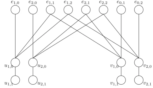
Fig. 1 The cover graph for an edgee=uvofGinP(G,3)

Construction of P(G,r)and the main gadgetLet(G,r)be an instance ofEquitable Coloring[tw] such that|V(G)|is divisible byr(if this is not the case, then this can be enforced by padding the instance with isolated vertices, see also [14]). We begin by constructing the poset P(G,r), which will play an important role later on. For every vertexv of V(G)we create 2(r−1)elements denotedvi,j, where 1 ≤ i ≤

r −1 and j ∈ {0,1}, such that the only dependencies in the poset between these elements are vi,1 ≤ vi,0 for all v ∈ V(G), for alli ∈ {1, . . . ,r −1}. For every

edgee = uv ∈ E(G)we creater2−1 pairwise-incomparable elementsei,j, such

that(i,j)∈({0, . . . ,r −1}2\{(0,0)}). The dependencies ofei,j are: ifi >0 then

ui,0≤ei,j, and if j >0 thenvj,0≤ei,j (see also Fig.1).

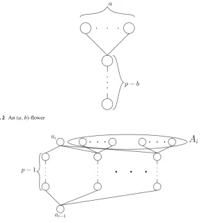
Construction of P(G,r,p)Let us now fix a prime number psuch that p does not dividee(P(G,r))andp>2r|V(G)| +r2|E(G)|. The main gadget in our reduction is a so-called(a,b)-flower, which consists of an antichain ofa vertices (called the petals) covering a chain ofp−belements (called thestalk); an illustration is provided in Fig.2. Due to Lemma2,(a,b)-flowers will later allow us to force a choice of exactly bvertices out ofa.

LetGbe a graph,rbe an integer and p be a prime number as above. Recall that |V(G)|is divisible byr and lets = |V(_rG)| (note that this implies that each color in an equitable coloring of Gmust occur precisely stimes in G). We proceed with a description of the posetP(G,r,p). The posetP(G,r,p)is split intor+3 “levels” L1, . . . ,Lr+3by linearly ordered elementsa0 ≤ a1 ≤ · · · ≤ ar+2 ≤ ar+3, called

theanchors. Each of these levels, besides Lr+3, will consist of some flowers and a

chain ofp−1 elements which we call astick; each of these flowers and the stick will always be pairwise incomparable. The anchorsa0andar+3are the unique minimum

and maximum elements, respectively. The stick and all the stalks of flowers in levelLi

will always lie between two consecutive elementsai−1andai, and the petals of these

flowers will be incomparable withai as well as some anchors above that (as defined

a

p−b

Fig. 2 An(a,b)-flower

p−1

ai−1

ai

_A

i

Fig. 3 Each level consists of a chain of lengthp−1 and a few flowers. The set of petals associated with levelLiis denoted byAi

We say that a flower (or its stalk, petals, or elements) isassociatedwith the level in which it is constructed, i.e., with the levelLisuch thatai−1≤c≤aifor stalk elements

candai−1≤dandd aifor petalsd. We denote the set of all petals associated with

levelLi as Ai (see Fig.3). For the construction, it will be useful to keep in mind the

following intended goal: whenever an(a,b)-flower is placed in leveli, it will force the selection of preciselybpetals (from its total ofapetals), where selected elements remain on leveli (i.e., betweenai−1andai) in the linear extension and unselected

elements are moved to levelr+2 (i.e., betweenar+2andar+3) in the linear extension.

We will later show that the total number of linear extensions which violate this goal must be divisible by p, and hence such extensions can all be disregarded modulop.

The firstrlevels are so-calledcolor classlevels, each representing one color class. We use these levels to make sure that every color class contains exactlys vertices. Aside from the stick, each such level contains a single(|V(G)|,s)-flower. Recall that the stalk and the stick on level 1≤i ≤rboth lie between anchorsai−1andai, and

levelLi with a unique vertexv∈V(G)and denote the petalvi. Each petalviwill be

incomparable with all anchors aboveai−1up toar+3, i.e.,vi aj fori ≤ j ≤r+2

andvi ≤ar+3. Intuitively, the flower in each color class level will later force a choice

ofsvertices to be assigned the given color.

Level Lr+1is called thevertexlevel and consists of one stick and |V(G)|-many

(r,1)-flowers; the purpose of this level is to ensure that every vertex is assigned exactly one color. Each flower is associated with one vertexv∈V(G)and we denote the petals of the flower associated with vertexv asvi for 1 ≤ i ≤ r. We setvi ≤ vi for all

v∈V(G)and 1≤i≤r.

LevelLr+2is called theedgelevel, and its purpose is to ensure that the endpoints

of every edge have a different color. It consists of a stick and|E(G)|-many(r2,1) -flowers. Each flower is associated with one edgee=uv ∈V(G)and we denote the petals of the flower associated witheasei,j for 1≤i ≤rand 1≤ j ≤r. Moreover,

for edgee=uvwe setui ≤ei,j,vj ≤ei,j, and we setar+2≤ei,jwheneveri= j.

Observe that this forces any petalei,i to lie betweenar+2 andar+3in every linear

extension (i.e., preventsei,i from being “selected”).

Level Lr+3is called thetrash level. It does not contain any new elements in the

poset, but it plays an important role in the reduction: we will later show that any petals which are interpreted as “not selected” must be located betweenar+2andar+3in any

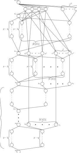
linear extension that is not automatically “canceled out” due to counting modulop. A high-level overview of the whole constructed posetP(G,r,p)is presented in Fig.4.

Establishing the desired properties ofP(G,r,p)andP(G,r)We begin by formaliz-ing the notion of selection. Let aconfigurationbe a partitionφof petals of all flowers intor+3 setsLφ₁, . . . ,Lφ_r+3. LetΦ denote a set of all configurations. We say that a linear extensionofP(G,r,p)respectsthe configurationφifLφ₁ a1 Lφ2

a2 · · · ar+2L_rφ₊₃and we denote the set of all linear extensions ofP(G,r,p)

that respectsφbyLφ_{. We say that a configurationφisconsistentifL}φ_{is non-empty;} this merely means thatLφ₁ ≤a1≤ Lφ₂ ≤a2≤ · · · ≤ar+2 ≤Lφ_r+3does not violate

any inequalities inP(G,r,p). Observe that ifφis consistent, thenLφ_{is exactly the set} of linear extension of the partial orderPφ_{(G,r,p), whereP}φ_{(G,r,p)is obtained by} enrichingP(G,r,p)with the relationsLφ₁ ≤a1 ≤ Lφ₂ ≤a2 ≤ · · · ≤ar+2≤ Lφ_r+3

and performing transitive closure (in other words,Pφ_{(G,r,p)is obtained by} enforc-ingφontoP(G,r,p)).

Since every linear extension ofP(G,r,p)respects exactly one configuration, it is easy to see thate(P(G,r,p)) =

φ∈Φ|Lφ| =

p−1 p−1

p−1 p−1

p−1 p−s

r

|V(G)| |V(G)|

r

|E(G)|

r2

u1 _v

1

ur vr

u1 _ur _v1 _vr

e1,1 e1,r er,1 er,r

ar+3

ar+2

ar+1

ar

ar−1

a1

a0

Let us first remark that for any configurationφ, the anchorsa0,a1, . . . ,ar+3are

comparable to all elements ofPφ_{(G,r,p). Now, letP}φ

Li be the poset induced by all

elementse∈Pφ_{(G,r,p)such thata}

i−1≤e≤ai ande=ai−1,e=ai. It is readily

seen thate(Pφ_{(G,r,p)) =} r+3

i=1e(P

φ

Li). We proceed by stating a series of claims

about our construction.

Claim 1 For each i∈ {1, . . . ,r}, it holds that either e(P_Lφ

i)≡0 mod p, or e(P

φ

Li)=

s!2p−1 p

and Lφ_i contains exactly s petals of Aiand no other petals.

Proof _{(of the Claim) Assume that}e(P_Lφ

i)≡0 mod pand recall that levelLicontains

a stick, which is a chain ofp−1 elements that is incomparable with all elements ofP_Lφ i

in every configurationφ. By Lemma2this implies that every connected component of

P_Lφ

idistinct from the stick has size divisible byp. Clearly,L

φ

i contains only those stalks

that are associated with the levelLi, and it contains all such stalks. It is readily seen

from the construction that any petal in∪j<iAjwould necessarily form a component of

size one inPφ_L

i. Hence,P

φ

Li contains only elements associated with levelLi, namely

elements of the stick and elements of a(|V(G)|,s)-flower. Moreover, by Lemma2

and the fact that|V(G)| +p−s <2p, each such flower has exactly pelements in levelPφ_L

i. Since thep−selements of the stalk must be inP

φ

Li, the posetP

φ

Li contains

exactlys elements of Ai. Clearly, the number of linear extensions of the petals of

the(|V(G)|,s)-flower inPφ_L

i iss!and hence by Lemma1e(P

φ

Li)=s!

2p−1 p

, which

concludes the proof. ⊓⊔

Claim 2 Either e(P_Lφ

r+1)≡0 mod p, or e(P

φ

Lr+1)=

(|V(G)|p+p−1)!

(p−1)!(p!)|V(G)| and L φ

r+1

con-tains exactly|V(G)|elements of Ar+1, specifically one petal for each(r,1)-flower on

level Lr+1.

Proof _{(of the Claim) Assumee(}P_Lφ

r+1)≡0 mod p, and let us first examine elements

that are not associated with levelLr+1. Clearly, no element associated with levelLr+2

can appear inP_Lφ

r+1and the only elements associated with any leveli <r+1 that can

end up inPφ_L

r+1 are petals. Each of these elements is smaller than exactly one petal at

levelLr+1and incomparable to all other elements associated with this level. It is easy

to see that largest possible size of a connected component ofP_Lφ

r+1isp−1+2r<2p.

By Lemma2, every connected component inPφ_L

r+1 (except for the stick) will have

size p, and thereforeP_Lφ

r+1 will contain exactly one element for every set of petals

associated withLr+1and no other elements. Hence,P_Lφ_r+1 consists of|V(G)|chains

of length pand one chain of length p−1. Thene(P_Lφ r+1)=

(|V(G)|p+p−1)!

(p−1)!(p!)|V(G)| follows

from Lemma1. ⊓⊔

Claim 3 Either e(P_Lφ

r+2)≡0 mod p, or e(P

φ

Lr+2)=

(|E(G)|p+p−1)!

(p−1)!(p!)|E(G)| and L φ

r+2

con-tains exactly|E(G)|elements of Ar+2, specifically one petal for each(r2,1)-flower

Proof _{(of the Claim) The idea of the proof is similar to the proof of the previous claim,} with one additional obstacle: that several flowers can be connected with petals from lower levels into one connected component on levelLr+2through the petals of flowers

on levelLr+1. So, assumee(Pφ_Lr+2)contains a connected componentCwhich contains

at least a single stalk. IfCcontains precisely the single stalk, then by Lemma2we have e(Pφ_L

r+2)≡0 mod p. Otherwise, for each stalk inC, there must be at least one petal

in the same flower (otherwise the stalk cannot be connected to the rest ofC); in other words, the intersection of each flower andCcontains at leastpvertices. Letadenote the number of flowers which intersectC,b2denote|Ar+2∩C|,b1denote|Ar+1∩C|

andb0denoteri=1|Ar∩C|. Then it follows that|C| = p·a+(b2−a)+b1+b0≤

p·a+r2|E| +r|V| +r|V|, and recall thatr2|E| +r|V| +r|V|<p. Furthermore, ifb1>0 (and at least one petal fromAr+1is required unlessCcontains only a single

flower), we havea · p < |C| < (a +1)· p. Hence any such C cannot have size divisible bypand by Lemma2we havee(P_Lφ

r+2)≡0 mod p. Otherwise, if no two

flowers are connected through a petal of a flower associated with level Lr+1, then

every connected component ofP_Lφ

r+2of sizepmust consist of a stalk and exactly one

petal and the claim follows analogously as the proof of Claim2. ⊓⊔

Claim 4 Ifφis a consistent configuration and for all i ∈ {1, . . . ,r+2}it holds that e(Pφ_L

i)≡0 mod p, then1)the petals in L

φ

r+1encode a proper equitable coloring

of V(G)where vertexv receives color i iff the petalvi lies in Lφi, and 2)P

φ

Lr+3 is

isomorphic withP(G,r).

Proof _{(of the Claim) From Claims 1, 2 and 3 together with the assumption that} e(Pφ_L

i)≡0 mod p, it follows that each of the levelsL

φ

1, . . . ,L

φ

r contains exactlys

petals associated with the corresponding level, levelLφ_r+1contains exactly one petal for each vertex ofGand levelLφ_r+2contains exactly one petal for each edge ofG.

For the first part of this claim, we observe that each pair of petals inLφ₁, . . . ,Lφr are

associated with distinct vertices ofG. If this were not the case, then since|V(G)| =r s there would exist a vertexv such that no element of Lφ₁, . . . ,Lφr is associated with

v. But due to the construction at levelr+1 there exists somei ∈ {1, . . . ,r}such thatvi ∈L_rφ₊₁. Then, sincevi ≤vi andvi can only occur either in levelLφi orL

φ

r+3

(the latter of which lies abovevi in the linear extension due to the configurationφ), this would lead to a contradiction. In particular, we conclude that there is a matching between the petals in levelr+1 (encoding the color for each vertex) and the union of petals in levels 1,2, . . .r(encoding the vertices assigned to each color class), and by Claim1it follows that there are exactlyspetals inLr+1associated with each color

class.

We now argue that the coloring is proper. Observe that by the same argument as above, if an edgee=uvsatisfiesei,j ∈L_rφ₊₂, thenui ∈Lφ_r+1andvj ∈L_rφ₊₁. From

the construction ofP(G,r,p)it follows that ifi = j, thenei,j ∈/ Lr+2. Combining

these two facts we get that the coloring encoded inLφ_r+1is indeed proper.

Now let us take a look at level Lφ_r+3. To prove the claim, we will construct an isomorphism f from elements ofP_Lφ

v ∈ V(G), precisely one elementvi ∈ L_rφ₊₁and precisely one of the firstr levels

contains an element associated withv; to be precise,vi ∈Lφ_i andvj ∈Lφr+3and hence

alsovj ∈ Lφ_r+3for allj =i. We set f(vj)=vj,0and f(vj)=vj,1, whenever j=i

and j <r. For the last remaining elements, we set f(vr)=vi,0and f(vr)=vi,1.

Next, for every edgee=uvthere is exactly oneea,b∈Lrφ+2. Moreover, ifea,b∈Lφr+2

thenua _{∈ L}φ

r+1andvb∈ L

φ

r+1, and all other petals for this edgeeare inL

φ

r+3. Let

gi(r) =i,gi(i)= 0, andgi(k)=k otherwise. Then we set f(ei,j) =ega(i),gb(j).

Observe that, sinceea,bdoes not lie inL_rφ₊₃, no edge is mapped to the non-existent

elemente0,0inP(G,r). It is straightforward to verify that f is really bijective mapping

between elements ofP_Lφ

r+3 andP(G,r). Moreover, f(u)≤ f(v)inP(G,r)if and

only ifu ≤ vinP_Lφ

r+3. Therefore,P

φ

Lr+3 is isomorphic withP(G,r)and the claim

holds. ⊓⊔

Claim 5 e(P(G,r,p)) ≡ 0 mod p if and only if e(P(G,r)) ·#EC(G,r) ≡ 0 mod p.

Proof _{(of the Claim) From previous claims and in particular Claim4, we already} know thate(Pφ_{(G,r,p))=0 mod ponly ifφcorresponds to an equitable coloring} ofG withr colors. Moreover, we know thate(Pφ_{(G,r,p)) =}r+3

i=1e(P

φ

Li)and if

e(Pφ_{(G,r,p))≡0 mod p, then}

r+3

i=1

e(P_Lφ i)= s!

2p−1 p

r _{(|V(G)|p+p−} 1)! (p−1)!(p!)|V(G)|

(|E(G)|p+p−1)!

(p−1)!(p!)|E(G)| e(P(G,r)).

Since p > |V(G)| + |E(G)|,(|V(G)|p +p−1)! is divisible by p|V(G)|, but not by p|V(G)|+1_{and(|E(G)|p+p−1)!is divisible by p}|E(G)|_{, but not by p}|E(G)|+1_.

Therefore, it is readily seen that

s! 2p−1 p

r _{(|V(G)|p+p−} 1)! (p−1)!(p!)|V(G)|

(|E(G)|p+p−1)! (p−1)!(p!)|E(G)|

is not divisible by p. We will denote this latter expression ascp; note thatcp

corre-sponds to the constantApintroduced at the beginning of this section. Hence, it is easy

to see that if #EC(G,r)denotes the actual number of equitable coloring ofGwithr colors, then

e(P(G,r,p))≡cpe(P(G,r))#EC(G,r) mod p.

Sincecpis not divisible by p, it is clear thate(P(G,r,p))≡0 mod pif and only

ife(P(G,r))·#EC(G,r)≡0 mod p, and the claim holds. ⊓⊔

Proof _{(of the Claim) Let us first upperbounde(}P(G,r))#EC(G,r). Clearly,P(G,r) contains m = 2(r −1)|V(G)| +(r2 −1)|E(G)| elements, hence e(P(G,r)) ≤ m!. It can easily be verified that the number of possibilities of dividing|V(G)| = r s vertices intor color classes with exactly s colors each is (₍r s_s!))r!. By Fact 1, the

product of all primes between 2r|V(G)| +r2|E(G)|and(2r|V(G)| +r2|E(G)|)2is at least(2r|V(G)| +r2|E(G)|)!22r|V(G)|+r2|E(G)|. However, 2(r−1)|V(G)| +(r2− 1)|E(G)| + |V(G)| ≤ 2r|V(G)| +r2|E(G)| and hence e(P(G,r))#EC(G,r) ≤ (2(r −1)|V(G)| +(r2−1)|E(G)|)! + |V_(s(G_!)r)|! is clearly less than the product of

all primes between 2r|V(G)| +r2|E(G)|and(2r|V(G)| +r2|E(G)|)2. Note that if a natural number N is divisible by set of primes p1, . . . ,pℓ then N is divisible by the product of these primes and in particular N is bigger than the product of these primes. Therefore,e(P(G,r))#EC(G,r)cannot be divisible by all primes between 2r|V(G)| +r2|E(G)|and(2r|V(G)| +r2|E(G)|)2, from which the claim follows.⊓⊔

Claim 7 tw(C(P(G,r,p)))≤r·(tw(G)+3)+6.

Proof _{(of the Claim) To distinguish vertices of}GandC(P(G,r,p))in this proof, we will refer to the vertices ofC(P(G,r,p))as elements. So, letT =(T,{Xt}t∈V(T))be a nice tree-decomposition ofGof width tw(G). UsingT, we show how to construct a tree-decompositionT′ _=(T′_,{X′

t}t∈V(T′₎)ofC(P(G,r,p))with treewidth at most r·(tw(G)+3)+6. The construction can be summarized as follows:

1. All bags ofT′will contain the anchorsa0, . . . ,ar+3as well as the top-most element

of each stalk of the(|V(G)|,s)-flowers in the firstrlevels; letδdenote this set of 2r+4 elements.

2. For every bagt∈T, the tree-decompositionT′will contain a nodet′such that if v∈Xt then{v1, . . . , vr} ∈X′t.

3. Afterwards, every introduce nodet ∈T that introduces a vertexvwill be replaced by a long pathPt which gradually introduces and subsequently forgets all

remain-ing elements associated with the flower ofvat levelr+1 (i.e., the stalk) as well as every petal from the firstrlevels associated withv.

4. For each edgee, we pick an introduce nodet ∈T which contains both endpoint ofeand extend the pathPt by a new segment which introduces and subsequently

forgets all elements associated with the flower ofeat levelr+2.

5. The root node is replaced by a path that takes care of all elements which are not associated with any vertex or edge inG.

Let us now take a closer look what happens in T′ whent ∈ T is an introduce node. Let v ∈ V(G) be the vertex introduced at t. Since X_t′ contains elements a0, . . . ,ar+2, v1, . . . , vr, and the maximum element of each stalk of the(|V(G)|,s)

-flower in the firstr levels, it is easily seen that every petal from the firstr levels associated withv as well as the stalk of the flower associated withvin level Lr+1

each forms a separate connected component ofC(P(G,r,p))\X_t′. Moreover, for an edgee = uv such that Xt contains both endpoints ofe, we have that X′t also

con-tains elementsu1, . . . ,ur and one can see that also the flower associated witheat level Lr+2 is a connected component ofC(P(G,r,p))\X′t. It is readily seen that

element from firstrlevels associated withv, the stalk of the flower associated withvin levelLr+1, and the flower associated withein levelLr+2for every edgeeintroduced

att. We then replaceX′_t by a path(Y1, . . . ,Yℓt)such thatYi =Bi ∪X ′

t and for each

i ∈ {1, . . . , ℓt−1}the node with bagYi+1is the parent of the node with the bagYi.

It is easy to see now, that when we are forgetting vertexv in nodetinT, we can forget elementsv1, . . . , vrinT′, because we already introduced all its adjacent edges inC(P(G,r,p))either in the path corresponding to the node ofT introducingvor the one introducing a neighbor ofv.

Finally, when we get to the root node ofT, we have already forgotten all elements associated with any specific vertex or edge ofG. Therefore, the only elements besides δwhich need to be included inT′_{are the remaining elements in the stalks in the first}

rlevels and the sticks in every level. However, it is easy to see that at this point they all form separate chains inC(P(G,r,p))\δ. Hence there once again exists a path-decomposition of width at most|δ| +2 which gradually introduces and subsequently forgets all of these elements.

One can readily see that the properties (T1), (T2), and (T3) are satisfied and we are only left with computing the width ofT′_{. By construction, every join and forget node}

inT will become a node inT′whose bag has size at mostr· |Xt| +2r+4. On the

other hand, every introduce node inT will become a path inT′, and the largest bag on this path has size at mostr· |Xt| +2r+6, from which the claim follows. ⊓⊔

Concluding the proof Let us summarize the fpt turing reduction used to prove The-orem1. Given an instance(G,r)of Equitable Coloring[tw], we loop over all primes psuch that 2r|V(G)| +r2|E(G)|< p < (2r|V(G)| +r2|E(G)|)2, and for each such prime we construct the posetP(G,r,p); from Claim6 it follows that if #EC(G,r)=0, then at least one such prime will not dividee(P(G,r))·#EC(G,r), and by Claim 7 the cover graph of each of the constructed posets P(G,r,p)has bounded treewidth. For each such posetP(G,r,p), we computee(P(G,r,p))by the black-box procedure provided as part of the reduction. If for any prime p we gete(P(G,r,p)) ≡0 mod p, then we conclude that(G,r)is a yes-instance, and otherwise we reject(G,r), and this is correct by Claim5. ⊓⊔

4 Fixed-Parameter Tractability of Counting Linear Extensions

This section is dedicated to proving our algorithmic result, stated below.

Theorem 2 #LEis fixed-parameter tractable parameterized by the treewidth of the incomparability graph of the input poset.

The proof of Theorem2is divided into two steps. First, we apply a transformation process to a path-decompositionQof small width (the existence of which is guaranteed by Corollary1) ofI(P)which results in a tree-decompositionT of I(P)satisfying certain special properties. The properties ofT are then used to prove thatIC(P)has

treewidth bounded by the treewidth ofI(P). In the second step, we construct an MSO formulation which enumerates all the linear extensions ofP usingIC(P), and apply

4.1 The Treewidth of Combined Graphs

We begin by arguing a useful property of separators in incomparability graphs.

Lemma 3 Let S ⊆ V(I(P)). Then for each pair of distinct connected components C1,C2 in I(P)−S, it holds that for any a1,b1 ∈ C1 and any a2,b2 ∈ C2 we

have a1 ≤ a2iff b1 ≤ b2. Namely, the poset contains a total order of all connected

components in I(P)−S.

Proof _{We begin by proving the following claim.}

Claim 8 Let a, b, c be three distinct elements ofPsuch that ab and both pairs a, c and b, c are comparable. Then a≤c iff b≤c.

Proof _{(of the Claim) Suppose that, w.l.o.g.,a≤candc≤b. Then by the transitivity}

of≤, we geta≤bwhich contradicts our assumption thatab. ⊓⊔

Now to prove Lemma3, assume for a contradiction that, w.l.o.g., there exista1,b1∈

C1anda2,b2∈C2such thata1≤b1andb2≤a2. LetQ1be ana1-a2path inI[C1].

By Claim8,a1 ≤ b1 implies that every elementq on Q1 satisfiesq ≤ b1, and in

particulara2≤b1. Next, letQ2be ab1-b2path inI[C2]. Then Claim8also implies

that each elementq′onQ2satisfiesa2 ≤q′. Sinceb2lies on Q2, this would imply

thata2≤b2, a contradiction. ⊓⊔

To proceed further, we will need some additional notation. LetT =(T,X)be a rooted tree-decomposition andt ∈T. We denote byL(t)the set of all vertices which occur in the “branch” ofT−tcontaining the rootr; formally,L(t)= {v∈ Xt′\X_t|t′ lies in the same connected component asrinT−t}. We then setR(t)=V(G)\(L(t)∪ Xt). We also letTtr denote the connected component ofT−twhich contains the root

r.

Next, recall that each connected component of the graph obtained after deletingXt

must lie in a subtree ofT −t (Fact3). Let Υt be the set of connected components

of (I(P)\Xt)∩ R(t). Recall that because of Lemma3, the components ofΥt are

totally ordered byP. We say that two components B1, B2 ∈ Υt areconsecutiveif

there is no elementv∈V(I(P))\(Xt∪B1∪B2)that is in between elements in these

components; formally, for everyvit holds that eitherv ≤bfor allb ∈ B1∪B2, or

v≥bfor allb∈ B1∪B2.

Ablockof a bag Xt is a maximum set of consecutive connected components in

(I(P)− Xt)∩ R(t); note that each block has a natural total ordering among the

contained components, given by Lemma3. We say that a nodet ∈ T haszblocks if there existzdistinct blocks of Xt. Blocks will play an important role in the

tree-decomposition we wish to obtain from our initial path-tree-decomposition of I(P). The following lemma captures the operation we will use to alter our path-decomposition.

Lemma 4 LetT =(T,X)be a rooted tree-decomposition of a graph G and let t ∈T be such that there are z blocks of Xt. Then there is a tree-decompositionT′(T′,X′)

satisfying:

2. The tree T′contains T_tr as a subtree which is separated from the rest of T′by t . 3. The degree of t in T′is z+1.

4. There exists a bijectionαbetween the z blocks of Xtand the z trees in T′−t other

than T_tr such that for each block B of Xt, we haves∈α(B)Xs′\Xt =B.

5. For each t′∈ N[t]\T_tr, we have Xt′ =X_t.

Proof _{It will be useful to observe thatT −T}r

t is a subtree ofT and in particular it

is connected. Consider the following construction ofT′_{. First, we copy all nodes of}

T_tr∪ {t}(along with their bags) intoT′_{, thus ensuring that Property2holds. Second,}

for each block B of Xt we make a copy TB of the tree T −Ttr, and connect the

nodetB _{corresponding tot inT\T}r

t by an edge to the nodet inT′. Moreover, for

each nodes ∈ T\T_tr we set X′

sB = Xs ∩(B∪ Xt). It is easy to verify that all of

the required properties are now satisfied, and it remains to show thatT′ is indeed a tree-decomposition.

We argue thatT′_{satisfies all three properties of tree-decompositions. Property (T1)}

follows directly from fact thatT was tree decomposition, and hence every vertex that does not occur in a bag inT_tr must occur in some bagXs for some nodes ∈T\Ttr;

then this vertex either also occurs in Xt or occurs in some block B and hence in

X′

sB. Property (T2) is also straightforward, since each vertex either does not occur

in any block or in exactly one block, and in both cases monotonicity follows from the monotonicity ofT and the construction. For the final Property (T3), we recall that there are no edges between the blocks ofXt; in particular every edgee=abin

I(P)[Xt ∪R(t)]is either contained inXt, goes between a vertex ofXt and a vertex

of some blockB, or is contained in some block B. In all three cases, it holds that if a,b ∈ Xs for somes ∈ T\Ttr, thene ∈ XsB for some block B. Therefore,T′is a

tree-decomposition and the proof is complete. ⊓⊔

We proceed by showing how Lemma 4 is applied to transform a given path-decomposition.

Lemma 5 LetQbe a nice path-decomposition of I(P). Then there is a rooted tree-decompositionT = (T,X)of I(P)with the following properties.T is rooted at a leaf r and Xr = ∅, the width ofT is at most the width ofQ, and for any node t ∈ T

with z>1blocks:

1. The degree of t in T is z+1.

2. There exists a bijectionαbetween the z blocks of Xtand the z trees in T′−t other

than T_tr such that for each block B of Xt, we have_s∈α(B)Xs\Xt =B.

3. For t′∈N(t)∩T_tr there exists a vertexvsuch that Xt′ =X_t\{v}, and furthermore t′has degree at most2and1block.

4. For each pair of neighbors t,t′∈T , it holds that|Xt\Xt′| + |X_t′\X_t| ≤1.

Proof _{Let us order the vertices of}I(P)in the order in which they were introduced inQ. We set the first leaf ofQto be the rootr, and observe thatXr = ∅sinceQis nice. We

1. For each pair of neighborst,t′∈T, it holds that|Xt\Xt′| + |X_t′\X_t| ≤1. 2. For each vertexuthat was already processed, the introduce node ofusatisfies the

conditions of the lemma.

3. Any nodetof degree greater than 2 is an introduce node of an already processed vertex.

Clearly, all invariant conditions hold forQrooted atr (the first invariant condi-tion follows by the fact thatQis nice, and the remaining two are satisfied trivially). Similarly, all invariant conditions hold after applying Lemma4on the first introduce nodet inQ. Indeed, note that sinceXr = ∅, we can assume w.l.o.g. thattis a child

ofr andXt = {v}for some vertexv. Then the first and third invariant condition is

immediately seen to hold; as for invariant condition 2, ifthas more than 1 block then applying Lemma4ensures thattsatisfies Conditions1,2, and4, while Condition3

holds sincet′=r.

For the induction step, suppose that the conditions hold in a tree-decompositionT

obtained by inductively applying Lemma4as above, and the first unprocessed vertex is v. Lettbe the unique node wherevis introduced, and letT′_{be the tree-decomposition}

we obtained by applying Lemma4onT andt.

It is easy to verify thatT′ then satisfies the desired Conditions1,2, and4 at the nodet by Lemma4. As for Condition3, sincet is the introduce node ofv and the first invariant condition holds inT, it is clear that fort′ ∈ N(t)∩T_tr it is the case that Xt′ = X_t\{v}. Moreover, t′ cannot be an introduce node, since thent′ would have to introduce an already processed vertex, which would imply thatXt′ =X_t due to our application of Lemma4on introduce nodes. So, let us consider the nodeson the uniquet′-rpath that is the closest introduce node tot′, and lets′be the neighbor ofson thes-t′path. Since no vertex was introduced on thes′-t′path, it follows that R(s′)=R(t′). Sinces′only has 1 block by the construction, it must be the case that t′also only has one block, and so Condition3also holds.

We proceed by arguing that the invariant conditions remain satisfied byT′_{. Since} Q was nice andT satisfied the first invariant condition, it is readily seen that the first invariant condition holds for all pairs of neighbors inT_tr as well as fort with all of its neighbors. IfsB ands′B are neighbors in a treeα(B)of T′−t, then by the construction in Lemma4there exists a pair of neighborss,s′ ∈ T\Tr

t such that

X′

sB =Xs∩(B∪Xt)andX ′

s′B =Xs′∩(B∪Xt). But then|X ′ sB\X

′ s′B|+|X

′ s′B\X

′ sB| =

|(Xs ∩(B ∪ Xt))\(Xs′ ∩(B ∪ X_t))| + |(X_s′ ∩(B ∪ X_t))\(X_s ∩(B ∪ X_t))| ≤ |Xs\Xs′| + |X_s′\X_s| ≤1 and the first invariant condition follows. As for the second invariant condition, notice that from the construction it follows that all the vertices that precedevin the order of introduction inQmust have been introduced in some node ofT_tr, and the application of Lemma4does not alter such introduce nodes for previously processed vertices. Finally, by the induction hypothesis all nodes ofT\T_tr have degree at most 2, therefore from the construction in Lemma4it is clear that all nodes inT′\(T_tr ∪ {t})also have degree 2. Since all introduce nodes of unprocessed vertices lie inT′\(T_tr∪ {t}), we conclude that the third invariant condition also holds inT′_.