Reference point hyperplane trees

Richard Connor

Department of Computer and Information Sciences, University of Strathclyde, Glasgow, G1 1XH, United Kingdom

[email protected]

Abstract. Our context of interest is tree-structured exact search in met-ric spaces. We make the simple observation that, the deeper a data item is within the tree, the higher the probability of that item being excluded

from a search. Assuming a fixed and independent probability pof any

subtree being excluded at query time, the probability of an individual

data item being accessed is (1−p)d_{for a node at depthd. In a balanced}

binary tree half of the data will be at the maximum depth of the tree so this effect should be significant and observable.

We test this hypothesis with two experiments on partition trees. First, we force a balance by adjusting the partition/exclusion criteria, and compare this with unbalanced trees where the mean data depth is greater. Second, we compare a generic hyperplane tree with a monotone hyperplane tree, where also the mean depth is greater. In both cases the tree with the greater mean data depth performs better in high-dimensional spaces. We then experiment with increasing the mean depth of nodes by using a small, fixed set of reference points to make exclusion decisions over the whole tree, so that almost all of the data resides at the maximum depth. Again this can be seen to reduce the overall cost of indexing. Furthermore, we observe that having already calculated reference point distances for all data, a final filtering can be applied if the distance table is retained. This reduces further the number of distance calculations required, whilst retaining scalability. The final structure can in fact be viewed as a hybrid between a generic hyperplane tree and a LAESA search structure.

1

Introduction and Background

Sections 1.1 and 1.2 set the context of metric search in very brief detail; much more comprehensive explanations are to be found in [4, 12]. Readers familiar with metric search can skim these sections, although some notation used in the rest of the article is introduced.

1.1 Notation and Basic Indexing Principles

required solution being the set{s←S|d(q, s)≤t}. In general|S| is too large for an exhaustive search to be tractable, in which case the metric properties of

drequire to be used to optimise the search.

In metric indexing,S is arranged in a data structure which allows exclusion of subspaces according to one or more of the exclusion conditions deriving from the triangle inequality property of the metric. As we refer to these later, we summarise them as:

pivot exclusion (a) For a reference point p ∈ U and any real value µ, if

d(q, p) > µ+t, then no element of {s ∈ S | d(s, p) ≤ µ} can be a

solu-tion to the query

pivot exclusion (b) For a reference point p ∈ U and any real value µ, if

d(q, p) ≤ µ−t, then no element of {s ∈ S | d(s, p) > µ} can be a solu-tion to the query

hyperplane exclusion For reference pointsp1, p2∈U , ifd(q, p1)−d(q, p2)> 2t, then no element of {s∈S |d(s, p1)≤d(s, p2)} can be a solution to the query

1.2 Partition Trees

By “partition tree” we refer to any tree-structured metric indexing mechanism which recursively divides a finite search space into a tree structure, so that queries can subsequently be optimised using one or more of the above exclusion conditions. These structure data either by distance from a single point, such as the Vantage Point Tree, by relative distance from two points, for example the Generic Hyperplane Tree or Bisector Tree. Many such structures are documented in [4, 12]. In our context we are interested only in the latter category as will become clear.

As there are many variants of both structures, we restrict our description to the simplest form of binary metric search tree in each category. The concepts extend to more complex and efficient indexes such as the GNAT [1], MIndex [10] and various forms of SAT trees [7, 8, 2, 3], here we are only concerned with the principles.

1.3 Balancing the Partition

To the above exclusion conditions, we add one more first identified in [6]:

hyperbola exclusion For reference pointsp1, p2 ∈U and any real valueδ, if

d(q, p1)−d(q, p2)>2t+δ, then no element of{s⊂S, d(s, p1)≤d(s, p2) +δ} can be a solution to the query

The addition of the constantδ means that for any pair of reference points, an arbitrary balance can be chosen when constructing the tree. An algebraic proof of correctness for this property follows the same lines as that for normal hyperplane exclusion.

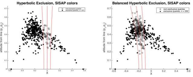
The purpose of this is illustrated in Figure 1. The diagrams show the two reference points p1, p2 plotted centrally along the X axisd(p1, p2) apart. Each other point is uniquely positioned according to its distances from p1 and p2 respectively. The data shown here is drawn from the SISAP colors data set under Euclidean distance.

Fig. 1.Balanced Hyperbolic Exclusion

mechanism is illustrated by the two outer lines, which show the boundaries of queries which allow the opposing semi-space to avoid being searched for possible solutions. If the distribution is representative, it is reasonable to use the same set of example points for both purposes.

On the left-hand side of the figure, normal hyperplane exclusion is illustrated. The data is split according to which is the closer reference point, which mani-fests here as either side of the Y axis. The exclusion condition is the hyperbola condition, depicted by the outer (hyperbolic) curves. Any query points outside these lines do not require the opposing semi-space to be searched.

However the partition of the data is unbalanced with respect to the chosen reference points. On the right hand side of the picture, the data set is split according to the central hyperbolic curve, the value for this being chosen to achieve an arbitrary balance of the data, in this case evenly divided. From the illustration it can be seen that fewer queries will achieve the exclusion condition; however, the magnitude of the space excluded will be greater in most cases.

For our purposes here, the point is that an even balance can be achieved in all cases, for arbitrary data and any reference points. Of course, unlike in a database indexing structure, an improved balance does not imply improved performance, and our working hypothesis at this point is in fact that balancing will, on whole, degrade performance as it reduces the mean depth of the data.

2

Balanced and Monotonous Partition Trees

Algorithms 1 and 2 give the simplest algorithms for constructing, and querying, a balanced partition tree.

Data:Si⊂S

Result: Node:< p1, p2:U, δ:R,left, right : Node>

selectp1, p2fromSi; if |Si|>2then

Si←Si− {p1, p2};

for allsj∈Sicalculated(sj, p1)−d(sj, p2);

find median valueδ;

create subsetsSl, Srsuch that ;

Sl={s←Si, d(s, p1)−d(s, p2)< δ}; Sr={s←Si, d(s, p1)−d(s, p2)≥δ};

left←CreateNode(Sl);

right←CreateNode(Sr);

end

Algorithm 1:CreateNode (balanced)

Data:q∈U, n: Node

Result: Result:{s∈S, d(s, q≤t})

Result ={};

if d(q, n.p1)≤tthen

Result.add(p1)

end

if d(q, n.p2)≤tthen

Result.add(p2)

end

if d(q, n.p1)−d(q, n.p2)≥2t+n.δ then

Result.add(Query(q,n.right))

end

if d(q, n.p2)−d(q, n.p1)>2t+n.δ then

Result.add(Query(q,n.left))

end

Algorithm 2:Query

1. The reference points need to be chosen carefully to be far apart, but also not to be very close to any reference point previously used at a higher level of the tree. Otherwise, in either case, few or no exclusions will be made at the node.

2. As well as relying on hyperbolic exclusion, each node can also cheaply store values for use, for both partitions, with both types of pivot exclusion. For both subtrees minimum and maximum distances to either reference point can be stored and used to allow pivot exclusion for a query. Most commonly, only the cover radius is kept for the reference point closest to the subtree. The minimum distance from the opposing reference point may also be of value; an interesting observation with the balanced tree, which can be seen by studying Figure 1, is that both these types of pivot exclusion may well function better with a higherδvalue at the node.

The monotonous hyperplane tree (MHT1_{) was first described in [9] where} it was described as a bisector tree using only pivot exclusion. The structure is essentially the same, but each child node of the tree shares one reference point with its parent, as shown in Algorithm 3. A significant advantage is that, for each exclusion decision required in an internal node of the tree, only a single distance needs to be calculated rather than two for the non-monotonous variant. The query algorithm is conceptually the same, but in practice the distance valued(q, p1) is calculated in the parent node and passed through the recursion to avoid its recalculation in the child node.

The intent behind this reuse of reference points was originally geometric in origin, based on an intuition of point clustering within a relatively low dimen-sional space; this intuition becomes increasingly invalid as the dimendimen-sionality of the space increases. Interestingly however the monotonous tree performs sub-stantially better that an equivalent hyperplane tree in high dimensional spaces.

1

Data:Si⊂S, p1∈S

Result: Node:< p1, p2:U, δ:R,left, right : Node>

selectp2 fromSi;

if |Si|>2then Si←Si− {p1, p2};

for allsj∈Sicalculated(sj, p1)−d(sj, p2);

find median valueδ;

create subsetsSl, Srsuch that ;

Sl={s←Si, d(s, p1)−d(s, p2)< δ}; Sr={s←Si, d(s, p1)−d(s, p2)≥δ};

left←CreateNode(Sl, p1);

right←CreateNode(Sr, p2);

end

Algorithm 3:CreateNode (monotonous balanced)

3

The Effect of Depth

As balance and monotonicity are orthogonal properties of the partition tree, we have now identified four different types of tree to test in experiments. At each node of each of the four trees described, it is not unreasonable to assume that over a large range of queries the probability of being able to exclude one of the subtrees is approximately constant.

Data is embedded within the whole tree. Viewed from the perspective of an individual data item at depth d within the tree, it sits at the end of a chain of tests, each of which may result in it not being visited during a query. The probability of any data item being reached, and therefore having its distance measured, is therefore (1−p)d, where p is the probability of an exclusion be-ing made at each higher node. It should therefore be possible to measure that (a) unbalanced trees perform better than balanced, and (b) monotonous trees perform better than non-monotonous, as in each case the mean data depth is greater.

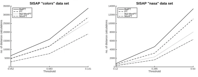
Figure 2 shows performance for the four tree types used for Euclidean search on the SISAPcolorsandnasa data sets [5]. In each case ten percent of the data is used as queries over remaining 90 percent of the set, at threshold values which return 0.01, 0.1 and 1% of the data sets respectively; results plotted are the mean number of distances required per query (n= 101414,36135 respectively.) The results presented are in terms of the mean number of distance calculations required per query; for most mechanisms over similar data structures execution times are proportional to these, and are not included due to space constraints2_. In all of these tests, a reasonable attempt to find “good” reference points is made; the selection of the first reference point is arbitrary (either randomly selected, or passed down from the construction of the parent node in the case of monotonous trees); the second reference point is selected as the point within

2 _{Source code to repeat these experiments, including timings, is available fromhttps:}

Threshold

0.052 0.083 0.131

no. of distance calculations

0 5000 10000 15000 20000 25000 30000

35000 SISAP "colors" data set

BalPT PT Bal-MonPT MonPT

Threshold

0.12 0.285 0.53

no. of distance calculations

0 2000 4000 6000 8000 10000 12000

14000 SISAP "nasa" data set

BalPT PT Bal-MonPT MonPT

Fig. 2.Four variants of hyperplane trees (monotonous or not, balanced or not) showing number of distances performed for SISAP benchmark searches. In each case, from the bottom (best) is: monotonous unbalanced, monotonous balanced, normal unbalanced, normal balanced

the subset which is furthest from the first. This works reasonably well, although performance can be improved a little by using a much more expensive algorithm at this point.

In each case, as expected, the balanced tree does not perform as well as the unbalanced tree, and the monotonous tree performs better than the non-monotonous tree.

4

Balancing and Pivot Exclusion

Before describing our proposed mechanism we briefly consider the effect on ex-clusion when relatively ineffective reference points are used. It should be noted that this will usually be the case towards the leaf nodes of any tree, as only a small set is available to choose from, and in fact this will affect the majority cases of any search in a high-dimensional space. In our particular context, we are going to compromise the effectiveness of the hyperplane exclusion through the tree nodes, by using relatively ineffective reference points, in exchange for placing the majority of the data at the leaf nodes.

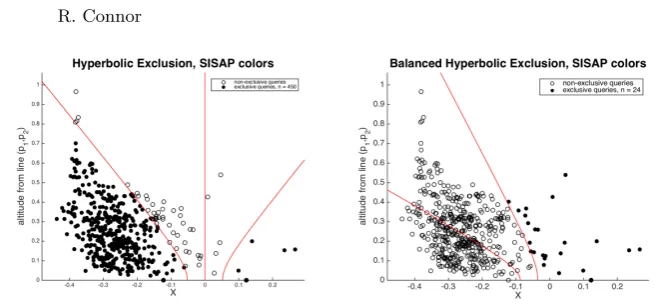
Fig. 3.The data as plotted in Figure 1, with a much worse choice of reference points. Note that in the right-hand chart, the pivots are so skewed that the left-hand branch

of the exclusion hyperbola does not exist in `22; the line on the left is the hyperbolic

centre of the data with respect to the reference points.

side, only 24 ex 500 queries allow exclusion, but in each case half of the data is excluded. So for this sample of points, treated as both data and query over the same reference points, both balanced and unbalanced versions save a total of around 6k distance calculations out of 25k.

However one further factor that can be noticed in general terms is that the use of pivot exclusion of both types (a cover radius can be kept for each reference point and semispace, and also the minimum distance between each reference point and the opposing semispace) may be more effective in the balanced version due to the division between the sets being skewed; it can be seen here that the left-hand cover radius in the balanced diagram is usefully smaller than the corresponding cover radius in the left-hand diagram.

This case is clearly anecdotal, and our experiments still show that on the whole the unbalanced version is more effective overall; however we believe this is because of the larger mean number of exclusion possibilities before reaching the data nodes. This is the aspect we now try to address.

5

Reference Point Hyperplane Trees

The essence of the idea presented here is to use the same partition tree structure and query strategy, but using a fixed, relatively small set of reference points to define the partitions. The underlying observation is that, given we can achieve a balanced partition of the data for any pair of reference points, we can reuse the same reference points in different sub-branches of the tree. Attempting the same tactic without the ability to control the balance degrades into, effectively, a collection of lists.

the mean depth traversed before another distance calculation is required will be greater.

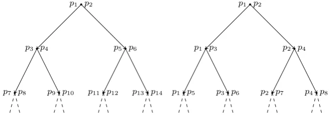
Assuming a balanced tree is constructed as above, the binary monotonous hyperplane tree stores half of its data at the leaf nodes, which have a depth of log2nforndata. The non-monotonous variant has only one-third of its data in the leaf nodes, and the mean depth is corresponding smaller. The two tree types are illustrated in Figure 4, where it is clear to see the average depth of a data item is always greater for the monotonous case. In fact empirical analysis shows that for large trees, the Reference Point tree has a weighted mean data depth of exactly one more than the Monotonous tree, which in turn has a weighted mean data depth of exactly one more than the non-monotonous tree.

p1 p2

p3 p4 p5 p6

p7 p8 p9 p10 p11 p12 p13 p14

p1 p2

p1 p3 p2 p4

p1 p5 p3 p6 p2 p7 p4 p8

Fig. 4.Generic and Monotonous Hyperplane Trees. Note the re-use of a single parent node for constructing the child node partition. For large trees, mean data depth is

log2n−1 for Generic, and log2nfor Monotonous.

To investigate this advantage further, we have considered two ways of using a small fixed set of points for the tree navigation, illustrated in Figure 5.

5.1 Permutation Trees

The first we refer to as a permutation tree. The underlying observation here is that, for a fixed set of nreference points, there exist n₂

unique pairs of points that can be used to form a balanced hyperplane partition. These can be assigned a numbering, as can the internal nodes of the tree, so that a different permutation is used at each node of the tree. At construction time, the permutation used for the particular node is selected and the difference of the distances to each point are calculated, the data is then divided into two parts based on the median of these differences. At query time, the distance between the query and each of the

n reference points can be pre-calculated; this gives all the information that is required to navigate the tree as far as the leaf nodes where the data is stored.

The strength of this method derives from the rate of growth of the function

n

2

p1 p2

p1 p3 p2 p3

p1 p4 p2 p4 p3 p4 p1 p5

p1 p2

p2 p3 p2 p3

p3 p4 p3 p4 p3 p4 p3 p4

Fig. 5.Permutation and Leanest trees. In either case, on scaling, mean data depth is

effectivelylog2n+ 1 as all data is stored at the leaf nodes.

aroundninternal nodes and therefore permutations, which in turn requires only around

√ 8n

2 reference points. This equates to around 1,400 points for 1M data, 14k for 100M data etc.

We have built such structures and measured them; the results are shown in Figure 6. They are encouraging; for the colors data set in particular, this is faster, and requires less distance calculations, than any other balanced tree format. It seems to do relatively better at lower relative query thresholds, and for the higher-complexity data of the colors data set. Finally, we should note that the reference points from which the permutations are constructed are, at this point, selected randomly; we believe a significant improvement could be obtained by a better selection of these points but have not yet investigated how to achieve this.

Threshold

0.052 0.083 0.131

no. of distance calculations

0 5000 10000 15000 20000 25000 30000

35000 SISAP "colors" data set

BalPT PT Bal-MonPT MonPT Permutation Tree

Threshold

0.12 0.285 0.53

no. of distance calculations

0 2000 4000 6000 8000 10000 12000 14000

16000 SISAP "nasa" data set

BalPT PT Bal-MonPT MonPT Permutation Tree

5.2 Leanest Trees

For our other test, we have selected a strategy that we did not expect to work at all; for a set ofn+ 1 reference points, we partition eachlevel of the tree with the same pair of points. That is, for the node at level 0, we use points {p0, p1} to partition the space; at level two, we use the pair {p1, p2}, etc. For all nodes across the breadth of the tree, for depthmwe use the reference pair{pm, pm+1}. This requires the selection of only log2n+ 1 reference points for data of sizen. For this strategy, it is much easier to provide relatively good pairs of points for partitioning the data, as there are relatively very few of them. For the results given we used a cheap but relatively effective strategy. The first reference point is chosen at random; repeatedly, until all are selected, another is found from the data which is far apart (in these cases we only sampled 500 points), and so on until all the required points are found. One further check is required, that none of the selected points is very close (or indeed identical) to another already selected, as that would result in the whole layer of the tree performing no exclusions at all.

5.3 Leanest Trees with LAESA

We have one more important refinement. The build algorithm for the Leanest Tree, for greatest efficiency, will pre-calculate the distances from the small set of reference points to each element of the data; this data structure can then be passed into the recursive build function as a table. This table has exactly the same structure as the LAESA [11] structure.

The table has onlynlog₂nentries and may therefore typically be stored along with the constructed tree. At query time, a vector of distances from the query to the same reference points is calculated before the tree traversal begins. Whenever the query evaluation reaches a leaf node of the tree, containing therefore a data node that has not been excluded during the tree traversal, a normal tree query algorithm would then calculate the distance between the query and the datum

sat this node. Ifd(q, s)≤tthensis included in the result set.

However, before performing this calculation (these distance calculations typ-ically representing the major cost of the search) it may be possible to avoid it, as for eachpi in the set of reference points,d(q, pi) andd(s, pi) are both available,

having been previously calculated. If, for anypi,|d(q, pi)−d(s, pi)|> t, it is not

possible thatd(q, s)≤t(by the principle of Pivot Exclusion (a) named in Section 1.1) and the datum can be discarded without its distance being calculated.

Threshold

0.052 0.083 0.131

no. of distance calculations

0 5000 10000 15000 20000 25000 30000

35000 SISAP "colors" data set

BalPT PT Bal-MonPT MonPT Leanest Tree Leanest Tree/LAESA adjusted L/L cost

Threshold

0.12 0.285 0.53

no. of distance calculations

0 2000 4000 6000 8000 10000 12000 14000 16000

18000 SISAP "nasa" data set

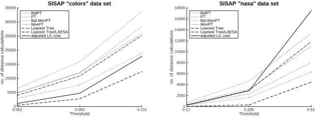
BalPT PT Bal-MonPT MonPT Leanest Tree Leanest Tree/LAESA adjusted L/L cost

Fig. 7.Cost of Leanest Tree indexing. The costs for the two datasets are plotted in bold against the background of the costs plotted in Figure 2 for comparison. The LAESA hybrid is the lowest line in each graph; this is not a true representation of overall cost, as explained in the text; the solid line gives a good estimate of the true cost of the hybrid mechanism.

6

Analysis

Figure 7 shows measurements for the Leanest Tree and its LAESA hybrid. These are plotted in bold, again set in the context of the greyed-out measurements copied from Figure 2.

In each case, the top dotted line is for the Leanest Tree measured without using the LAESA hybrid. This is comparable to the Permutation Tree, and again it is worth noting that this is a good performance for a balanced tree; in cases where balancing is required, for example if the data does not fit in main memory and requires paging, this mechanism is worthy of consideration.

The lower dotted line is the raw number of distance measurements made by the hybrid mechanism. This is by far the best performance measured in these terms for both data sets; however, for reasons explained above, it must be noted that this does not represent actual measured performance in terms of query time, as there is a significant extra cost entailed in performing the LAESA-based filtering. In some cases however the number of distance calculations will swamp any other cost of the query and this line would be representative for the mechanism.

LAESA exclusion is attempted, 0.8 of a distance calculation is added to the total measured from the original space. For thecolors data, these figures are 17 and 118 respectively, giving a much lower, if still pessimistic, adjustment.

It may be noted that the total number of distance measurements made by this mechanism is similar (although in general smaller) to that required by the pure LAESA mechanism; however, a query using LAESA requires a linear scan of the whole LAESA table, whereas our hybrid mechanism resorts to using the LAESA table only for data which has not already been excluded through the tree traversal, and therefore retains scalability.

The main outcome of our work is thus represented by the solid black line in the left hand figure, which give a substantially better better performance for this data set than any other we are aware of. The hybrid Leanest/LAESA mechanism appears to be very well suited for data sets which are very large and require paging, whose individual data items are very large, or whose distance metrics are very expensive.

7

Conclusions and Further Work

Having made the observation that the monotonous hyperplane tree is substan-tially more efficient that the non-monotonous equivalent, even in high-dimensional spaces, we formed the hypothesis that this is primarily due to the longer mean search paths to each data item. We have taken this idea to its extreme, in con-junction with an ability to force balance onto a hyperplane partition, through the design of “permutation” and “leanest” hyperplane trees. In particular, the latter requires onlylog2n+ 1 reference points for data of sizen, therefore leaving effectively all of the data at the leaf nodes of the tree. We have tested both mechanisms against two SISAP benchmark data sets, and found good realistic performance in comparison with other structures that are balanced and there-fore usable for very large data sets, or very large data points, which require to be paged.

Furthermore we note that the balanced tree mechanism can also be viewed as a scalable implementation of a LAESA structure, giving very good performance in particular for high-dimensional and expensive distance metrics. For very little extra cost, LAESA-style filtering can be performed on the results of the tree search, apparently giving the best of both worlds. We continue to investigate this mechanism in metric spaces more challenging that the benchmark sets reported so far.

8

Acknowledgements

the anonymous referees. Thanks also to Jakub Lokoˇc for pointing out his earlier invention of parameterised hyperplane partitioning!

References

1. Brin, S.: Near neighbor search in large metric spaces. In: 21th International

Confer-ence on Very Large Data Bases (VLDB 1995) (1995),http://ilpubs.stanford.

edu:8090/113/

2. Ch´avez, E., Ludue˜na, V., Reyes, N., Roggero, P.: Faster proximity searching with

the distal SAT. In: Traina, A.J.M., Traina, C., Cordeiro, R.L.F. (eds.) Similarity Search and Applications - 7th International Conference, SISAP 2014, Los Cabos, Mexico, October 29-31, 2014. Proceedings. pp. 58–69. Lecture Notes in Computer Science, Springer International Publishing (2014)

3. Ch´avez, E., Ludue˜na, V., Reyes, N., Roggero, P.: Faster proximity searching with

the distal SAT. Information Systems pp. – (2016)

4. Ch´avez, E., Navarro, G.: Metric databases. In: Rivero, L.C., Doorn, J.H.,

Fer-raggine, V.E. (eds.) Encyclopedia of Database Technologies and Applications, pp. 366–371. Idea Group (2005)

5. Figueroa, K., Navarro, G., Ch´avez, E.: Metric spaces library. www.sisap.org/

library/manual.pdf

6. Lokoˇc, J., Skopal, T.: On applications of parameterized hyperplane partitioning.

In: Proceedings of the Third International Conference on SImilarity Search and

APplications. pp. 131–132. SISAP ’10, ACM, New York, NY, USA (2010), http:

//doi.acm.org/10.1145/1862344.1862370

7. Navarro, G.: Searching in metric spaces by spatial approximation. The VLDB Journal 11(1), 28–46 (2002)

8. Navarro, G., Reyes, N.: String Processing and Information Retrieval: 9th Inter-national Symposium, SPIRE 2002 Lisbon, Portugal, September 11–13, 2002 Pro-ceedings, chap. Fully Dynamic Spatial Approximation Trees, pp. 254–270. Springer Berlin Heidelberg, Berlin, Heidelberg (2002)

9. Noltemeier, H., Verbarg, K., Zirkelbach, C.: Data structures and efficient algo-rithms: Final Report on the DFG Special Joint Initiative, chap. Monotonous Bisector* Trees — a tool for efficient partitioning of complex scenes of geomet-ric objects, pp. 186–203. Springer Berlin Heidelberg, Berlin, Heidelberg (1992),

http://dx.doi.org/10.1007/3-540-55488-2_27

10. Novak, D., Batko, M., Zezula, P.: Metric index: An efficient and scalable solution for precise and approximate similarity search. Information Systems 36(4), 721 – 733 (2011), selected Papers from the 2nd International Workshop on Similarity

Search and Applications{SISAP}2009

11. Ruiz, E.V.: An algorithm for finding nearest neighbours in (approximately)

con-stant average time. Pattern Recognition Letters 4(3), 145 – 157 (1986), http:

//www.sciencedirect.com/science/article/pii/0167865586900139