Optimisation of offshore wind farms using a genetic algorithm

Optimisation of Offshore Wind Farms Using a Genetic Algorithm

Industrial Doctorate Centre in Offshore Renewable Energy, The University of Edinburgh Edinburgh, United Kingdom

Dr. John Chick

Institute for Energy Systems, The University of Edinburgh Edinburgh, United Kingdom

Prof. Lars Johanning

College of Engineering, Mathematics, and Physical Sciences, University of Exeter Penryn, United Kingdom

Dr. Mahdi Khorasanchi

Department of Naval Architecture, University of Strathclyde Glasgow, United Kingdom

Sebastien Pelissier EDF Energy R&D UK Centre

London, United Kingdom

A modular framework for the optimisation of an offshore wind farm using a discrete genetic algorithm is presented. This approach uses a bespoke grid generation algorithm to define the discrete positions that turbines may occupy thereby implicitly satisfying navigational and search and rescue constraints through the wind farm. The presented methodology takes a holistic approach optimising both the turbine placement and intra-array cable network, while minimising the levelised cost of energy and satisfying real world constraints. This tool therefore integrates models for the assessment of the energy production including wake losses; the optimisation of the intra-array cables; and the estimation of costs of the project over the lifetime. This framework will allow alternate approaches to wake and cost modelling as well as optimisation to be benchmarked in the future.

KEY WORDS: offshore wind farm layout optimisation; genetic algorithm

INTRODUCTION

With the growth of the offshore wind sector and the development of large offshore wind farms in the coming years, it has become an important point to ensure that the wind farms are developed in such a way as to maximise their potential. In order to meet this need, the field of wind farm layout optimisation has been in development since the seminal paper by Mosetti, Poloni, and Diviacco (1994). Though this field has been in development for the past twenty years, there still remains much work before layout optimisation displaces the industry standard rules-of-thumb approach to layout design. This paper presents a new framework that has been developed to address the layout optimisation problem with the goal of ultimately developing a tool that would be deployed by wind farm site developers.

This framework takes a holistic approach to layout optimisation based around the objectives and constraints that would be faced by an

offshore wind farm developer in the UK. This approach introduces a generalised means of discretising the wind farm area in such a way that a grid of potential turbine positions is first generated. The use of this grid ensures that the final turbine positions which are selected from this grid satisfy the requirement of having turbines along straight lines.





 







t t

t n

t t

t

r

AEP

r

C

LCOE

1 1

)

1

(

)

1

(

(1)

where 𝐶𝑡 are the costs incurred in year 𝑡, 𝑛 is the project lifetime time,

𝐴𝐸𝑃𝑡 is the annual energy production (AEP) in year 𝑡, and 𝑟 is the

discount rate of the project. The LCOE measured in £/MWh effectively gives a measure of the cost effectiveness of the layout proposed and therefore acts as a means to compare the layouts under consideration on a relative basis.

Existing approaches do not apply tools and methodologies that have considered all the constraints faced by a developer, nor do they consider the full impact the layout has on the LCOE. Many of the previous studies opted to use simpler cost models thereby ignoring the effect the layout has on costs (Mosetti et al. 1994, Grady et al. 2005). The studies that have considered detailed cost models however, have not considered the full set of constraints that a developer would be faced with (Elkinton 2007, Larsen et al. 2011, Larsen and Réthoré 2013). The tool developed as part of this work seeks to reconcile this by including both detailed models for assessing the layout dependent elements as well as a full set of constraints in order to generate layouts which would be acceptable from a developer perspective.

The work presented has developed a flexible framework by which the energy, cost, and electrical infrastructure are assessed independently for each layout. Due to the modularity, alternate wake, cost, or electrical infrastructure models can easily be implemented in the future for comparison purposes and sensitivity studies. The approach presented has also included constraints for maintaining navigation channels through the sites, minimum separation between turbines, and seabed restrictions, constraints that are less frequently seen in existing tools. The tool also generates an optimised intra-array electrical configuration simultaneously satisfying not only seabed constraints, but also cable capacity, cable crossing, and junction box capacity constraints.

A GA with bespoke crossover and mutation operators has been developed and applied successfully to this problem. The modular platform constructed would allow other optimisation algorithms such as particle swarm, ant colony optimisation, or simulated annealing to be implemented using the same evaluation function and tool approach. This paper summarises the initial application of this holistic approach to layout optimisation of offshore wind farms. The optimisation framework is applied to a hypothetical wind farm made up of 30 wind turbines in order to demonstrate the capabilities of the approach. The discussion section explores further improvements that will be made to the framework to increase the relevance to a wind farm developer. METHODS

As this tool has been developed as part of a larger project which seeks to assess the suitability of different wake models, cost models, optimisation objectives, and optimisation algorithms, it has intentionally been designed to be as flexible as possible while also adhering to the realistic challenges which would be faced by a project developer.

Grid Generation

In the UK, project developers have been urged to use symmetric layouts with turbines placed along a regular grid in order to comply with the navigational safety and search and rescue requirements (NOREL Group 2013). Rather than defining navigational channels, this constraint has been proposed as requiring the turbines to be placed in straight lines with no deviation from these lines. As a result of this, most optimisation approaches have limited the optimisation process to specifying the regular spacing between turbines. The tool developed here, however, looks instead to give the optimiser greater freedom by designing a grid which has more potential turbine positions than there are turbines to place. This allows the optimiser to change the spacing between turbines throughout the wind farm while still keeping the turbines in straight lines. It is believed that even though this creates a regular grid with holes, the final layout will still satisfy the navigational requirements.

The first step in this optimisation approach is therefore to produce this grid of potential turbine positions. To do this, the tool first identifies the dominant wind direction based on the wind rose describing the wind resource at the site and converting this to an energy rose representing the kinetic energy flux of the wind and the relative occurrence of the wind speed and wind direction combination. The dominant wind direction is then defined as the weighted circular mean of the wind direction sector where the wind direction is weighted by the kinetic energy flux. The dominant wind direction, once identified will act as one of the principle axes along which the grid of points is generated. By aligning the principle axis with the dominant wind direction, the optimiser will be able to align turbines in rows perpendicular to the dominant wind direction, thereby minimising the interaction of wakes. At the same time, having a large grid with more possible positions than turbines to be placed allows the optimiser to introduce space for wakes to recover where necessary. This approach also allows the optimiser flexibility in adjusting the spacing relative to each individual turbine rather than for the entire wind farm.

Once the dominant wind direction is identified, the algorithm expands and contracts the spacing as necessary until a grid with the desired number of valid turbine positions is generated. For each spacing, the grid is produced with a fixed ratio between downwind and crosswind spacing. After this each point is checked to ensure that it satisfies the geographical information system (GIS) constraints of where turbines can be placed. If after this, it is found that:

a) insufficient grid points are in valid positions, then the spacing is decreased, and the process repeated;

or

b) too many grid points exist, then the spacing is increased, and the process is repeated.

The desired number of grid positions is treated as a minimum and a small tolerance of the range of 10% is introduced to ensure that a valid grid can always be generated. In this way, “too many” is defined as more grid points present than the desired range, and likewise “insufficient” refers to grids which have fewer valid turbine positions than desired.

Annual Energy Production

assessment in turn can be said to be made up of two components, an understanding of the wind resource at the site, and modelling of potential wakes behind each proposed turbine.

Any device which extracts energy from a natural flux such as the wind is known to directly impact and alter the natural flux as a result of the energy extraction. In the case of wind turbines, the wake behind a wind turbine is characterised by lower extractable wind speeds, but higher levels of turbulence intensity (Barthelmie et al. 2006, 2009, Burton et al. 2011). These wakes are also known to interact with one another leading to a more significant reduction in available energy as a result of the superposition of multiple upwind wakes (Katic et al.

1986, Schlez and Neubert 2009).

Wake models, can broadly be categorised into two categories: analytic wake models and field models. Analytic wake models are simpler models while field models are generally based on solving the Navier-Stokes equations. Though the annual energy production module can either be run independently or as part of the optimisation tool, it was decided to use an analytic wake model as opposed to a field model to predict the wakes, as this results in substantially quicker computational times (Renkema 2007, Sanderse et al. 2011).

Previous work by the authors (Pillai et al. 2014) as well as other studies (Gaumond et al. 2012) had shown that for existing wind farms, the Larsen model (Larsen 1988) represents a good balance between accuracy and computational complexity when compared to a) the Jensen/PARK model (Katic et al. 1986), b) the Ishihara model (Ishihara et al. 2004, Crasto and Castellani 2013), and c) the Ainslie eddy-viscosity model (Ainslie 1988, Anderson 2009). The Larsen model is an analytic model based on a closed-form solution of the Reynolds-Averaged Navier Stokes (RANS) equations and Prandtl mixing theory (Larsen 1988, Renkema 2007). For this study, the Larsen model has therefore been deployed, however, other wake models can easily be implemented if need be.

In order to assess the AEP, the wind distribution at the site is used to determine the frequency of occurrence for each wind speed/direction combination. For each of these bins, the turbines in the layout are sorted such that the first turbine is the turbine furthest upwind. For each turbine, the free wind speed is then updated to account for the wakes created by any upwind turbines and the superposition of these wakes. The variation in power generation and thrust coefficient are considered based on the modified wind speed as a result of the wake effect and bins are generated related to speed and directionality. The aggregate power generated for the entire layout for these bins, are then multiplied by the frequency of this wind speed and direction combination. The sum of each of these powers for the bins represents the AEP for the proposed layout. This approach is similar to that taken by other tools and AEP computations (Mosetti et al. 1994, Grady et al.

2005, Elkinton 2007, Pérez et al. 2013, DNV GL - Energy 2014). Electrical Infrastructure Optimisation

Previous layout optimisation tools have generally assumed a constant inter-turbine spacing, and therefore the changes in total cost due to the intra-array cables are not characterised. However, as the layout changes, the total length of infield cable required can change quite significantly thereby affecting the costs. As the turbine layout has a direct impact on the cable layout it is important for a layout optimisation tool to take this into account.

This tool therefore implements an intra-array cable optimisation tool

in order to determine the cost of the electrical system for each turbine layout under consideration.

The authors have previously developed an optimisation methodology for optimising the intra-array cable network of an offshore wind farm (Pillai et al. 2015). This approach accounts for real wind farm planning constraints in order to determine the optimal positions for the necessary offshore substations and then designs an intra-array collection network which minimises both the cost and the peak losses. The optimisation tool first determines the optimal positions of the substations based on a modified ‘kmeans++’ algorithm. Kmeans++ is a modified version of the commonly used kmeans clustering algorithm which uses a weighted-random approach to seed the initial cluster centres resulting in both better solutions and quicker runtimes than the original kmeans algorithm (MacQueen 1967, Arthur and Vassilvitskii 2006). For this tool, the kmeans++ algorithm is further constrained to account for the capacity constraints of each substation and the fact that within the wind farm area, there are regions where substations cannot be placed. From here, a pathfinding algorithm based on Delaunay Triangulation is used to determine possible cable paths for each turbine and the respective cost of these paths. The pathfinding algorithm is used to account for the areas in which cables cannot be laid due to seabed constraints and obstacles. Finally, a capacitated minimum spanning tree (CMST) is constructed based on the cable costs found in the pathfinding step. The CMST represents the optimal network and is solved using Gurobi, a commercial mixed-integer linear programming (MILP) software. An iterative approach is taken in order to eliminate any cable crossings in the solution.

This tool has previously been applied to large wind farms and has been found to offer significant reductions in the total cable needed when compared to industry standard approaches (Pillai et al. 2015). Cost Assessment

Previous works that have included a cost breakdown typically have not been able to validate their cost models and as a result have introduced significant uncertainty into the optimality of their solutions (Elkinton 2007, Fagerfjäll 2010). As this tool has been developed in conjunction with EDF Energy R&D UK Centre, it has been possible to directly develop and validate the cost assessment methodologies. Consequently this work presents costs that have been parameterised and validated against real costs expected to be incurred by large offshore wind farms deploying wind turbines in the 5-8 MW range in UK waters.

The total cost of the wind farm is broken down into eight major cost elements:

1. Turbine Supply 2. Turbine Installation 3. Foundation Supply 4. Foundation Installation

5. Intra-array Cables (Supply & Installation) 6. Decommissioning

7. Operations and Maintenance (O&M) 8. Offshore Transmission Assets

Turbine installation. The turbine installation costs are based on market values for vessel costs and capacities and are modelled by first modelling the total amount of time needed to install all the turbines at their specific locations. This includes not only the computation of the travel time between the turbines, but also the necessary time to go to and from the construction port. To calculate this, the turbines are clustered based on the capacity of the installation vessel, and for each cluster a shortest path is computed between the port, each turbine in the cluster, and the port again. This approach therefore accurately computes the distance that the vessel must travel over the installation process. From this, the total time is computed based on assumed weather availability and the costs computed based on the vessel and equipment day rates. The turbine layout, therefore, has a direct impact on the time needed to travel between turbine positions as well as to and from the port.

Foundation supply. Foundation costs are found to be highly dependent on the site conditions where the foundation is to be installed. To account for this dependence, previous cost models have attempted a bottom up approach based on the soil characteristics at the installation site to model the costs. Unfortunately this approach has proven difficult to validate for all foundation types (Elkinton 2007). For this tool therefore, a depth dependency has been developed from discussions with manufacturers and the specific soil conditions are not included. Larger turbines in the 5-8 MW range are more likely to use jacket foundations which have been found to be less sensitive to the soil conditions than to the depth (Elkinton 2007). Detailed bathymetry of the site is therefore necessary in order to accurately estimate the variation in foundation supply costs as a function of the turbine layout. For a jacket foundation, the cost from discussions with manufacturers was found empirically to follow the below non-linear relationship:

𝐶𝑓𝑜𝑢𝑛𝑑𝑎𝑡𝑖𝑜𝑛∝ 𝐷0.7574 (2)

Foundation installation. The foundation installation process like the turbine installation module is based on estimating the time needed to complete the operations and converting this time to a cost. Unlike the turbine installation though, this is modelled as three distinct phases which each uses a different vessel to complete.

Regardless of the foundation type (gravity-based, monopile, or jacket), some seabed preparation is necessary. For a gravity-based foundation this might be the necessary dredging and levelling of the seabed, while for monopiles and jackets this would more likely be pre-pilling works including surveying and drilling. After this step, the foundations will be installed as a separate operation following which some kind of scour protection will often be added. The installation of scour protection is again modelled as a separate step involving a different vessel from either the site preparation or foundation installation processes. In some conditions, the scour protection will not be necessary, however, for the time being this model has assumed that all turbines will require scour protection.

Intra-array cable costs. The total horizontal length of intra-array cables required is computed from the intra-array cable optimisation tool described earlier. This tool is described in detail in previous work by the authors (Pillai et al. 2015). This tool has the support for optimising the layout for different cable cross-section sizes and therefore can output not only the total length of cable, but the horizontal lengths required for each segment and the required cross-section. From this, the intra-array cable cost module computes the necessary vertical cable and the necessary spare cable before computing the costs.

Following the calculation of the supply cost, the installation cost is computed in a similar manner to the turbine and foundation installation modules. This is done based on data available for cable trenching vessels and therefore assumes that all cables are trenched and buried.

Decommissioning. The decommissioning costs include the removal of the turbines and foundations. At the moment, it is unclear what will happen to the transmission and export cables. The model therefore assumes that these cables are not removed at the time of decommissioning, but simply cut at the turbines and substation, leaving the buried lengths as they are. The decommissioning costs are therefore modelled similar to the installation processes with the time each vessel is required first computed before this is converted to a cost. Like the installation processes it is assumed that the vessels have some finite capacity and must return to the decommissioning port during the overall operation. The turbines and foundations are assumed to be decommissioned in separate steps requiring separate vessels. Like the installation phases, this term is therefore dependent on the turbine positions and is affected by the proposed layout.

Operations and Maintenance. The operations and maintenance costs are based on a tool developed by EDF Energy R&D UK Centre which models the anticipated operations and maintenance cost of a project to vary with the project’s distance from the operations and maintenance port and the capacity of the project. As this term is affected by distance of the wind farm to the operations and maintenance port, this too is affected by the layout. The operations and maintenance costs are classed as operational expenditure (OPEX) as these are incurred each year of operation as opposed to the preceding cost elements which are only incurred during the construction period and are therefore classed as CAPEX elements.

Offshore Transmission Assets. The final cost element of this cost model is the inclusion of the offshore transmission assets and the offshore transmission asset transfer fees. In the UK, the offshore substation, export cables, and onshore substation must be owned and operated by a separate company from the wind farm operator. Practically, therefore, most wind farm developers build these assets, and then transfer them to a transmission operator before commissioning the wind farm. As a result, only some of the CAPEX is incurred by the project, and the rest is incurred as a component of the transmission fee along with regionally based costs set by the network operator, in the UK this is National Grid. Both the CAPEX and OPEX components of the Offshore Transmission Owner’s assets have been computed in discussion with National Grid and equipment manufacturers based on the capacity of the assets.

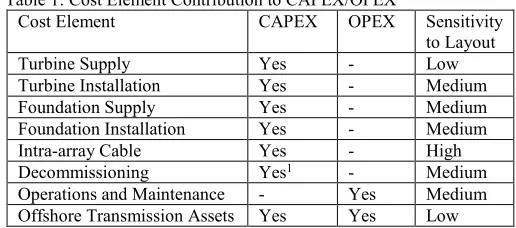
Table 1: Cost Element Contribution to CAPEX/OPEX

Cost Element CAPEX OPEX Sensitivity

to Layout

Turbine Supply Yes - Low

Turbine Installation Yes - Medium

Foundation Supply Yes - Medium

Foundation Installation Yes - Medium

Intra-array Cable Yes - High

Decommissioning Yes1 _{- Medium}

Operations and Maintenance - Yes Medium Offshore Transmission Assets Yes Yes Low

Constraints

An important step for all optimisation routines is to clearly define the constraints which must be applied and which limit the solution space. In this case, the intra-array cables are optimised as part of the evaluation function for the larger turbine placement problem, and there are a number of constraints to be considered just for this sub-problem separate from those which explicitly constrain the turbine placement.

First, the site boundary defines the area in which turbine foundations can be placed. As developers are required to keep the entire wind turbine within their leased turbine area, the boundary is adjusted using GIS software to include the necessary “negative buffer” to account for the size of the turbine blades. The boundary used by this tool therefore represents a smaller region than the overall turbine area.

Second, within the site there may be areas containing unexploded ordnance (UXOs) or wrecks. These areas generally cannot contain turbines or cables and are therefore treated as exclusion areas by the optimiser. Similarly, turbines can generally not be placed in areas where the seabed slope is too steep. Generally, areas over 5% slope will be considered as too steep for turbines and are similarly treated as exclusion areas. All areas also have an additional 50 m buffer area. By using the grid generation method, these placement constraints are implicitly satisfied for the turbines within the wind farm and need only be considered for the substation and intra-array cables.

Third, the turbines generally need to be a minimum distance away from one another, for safety and navigational reasons. These are generally given as exclusion circles around each turbine, however, consenting bodies may alternatively give separate downwind and crosswind distances defining an exclusion ellipse. These ellipses will generally require more significant separation in the downwind direction than in the crosswind direction.

Finally, in the case of most UK offshore wind farms, consenting bodies have stipulated that the layout of turbines in offshore wind farms should have some degree of uniformity to ensure safe passage through the farm as well as not act as a hindrance to search and rescue operations (NOREL Group 2013). This constraint is explicitly satisfied by the grid generation approach prior to execution of the GA. By doing this, a clear grid is defined on which turbines can be placed. As this constraint is already considered, it is not implemented within the framework of the GA.

The intra-array cable optimisation also has a number of constraints unique to its sub-problem. These include not only that the cables and the substations must be within the turbine area and may not enter the exclusion areas (seabed slope is not an exclusion area for cables), but also that power cannot be stored at a turbine and therefore the intra-array cable network must be balanced; turbines have a limited number of connection points and therefore a maximum number of cables that connect to a turbine exists; cables may not intersect except at the substation or at turbines; and cables have a finite capacity which cannot be exceeded (Pillai et al. 2015).

Genetic Algorithm

GAs are a type of population based evolutionary algorithms that are well suited to a variety of problem types (Holland 1992). GAs have previously been deployed for optimising offshore wind farm layouts and have generally been found to offer good solutions to the problem

at hand (Elkinton 2007, Guillen 2010, Larsen et al. 2011).

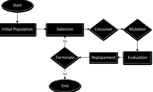
GAs are so named as they borrow from biological evolution and have analogous algorithms to genetic principles. In a GA, the solutions are thought of as genomes with each turbine position thought of as gene. GAs operate on a population basis that is to say that a population of solutions is considered in which the best solutions have a higher probability of passing on genes to members of the next generation. The flowchart in fig. 1 outlines the operating principles of a GA and the steps involved. The unique aspect of the GA at hand is that rather than implementing a generic GA and then testing for compliance within the evaluation function, the crossover and mutation steps have been designed specifically to include the constraints. In this case, because a predefined grid has been created during the grid generation step, the genes of the GA are binary and represent the presence of a turbine at the specific grid locations; one gene per grid location. For the implementation at hand, the problem was formulated as a minimisation problem in which the fitness of an individual was given by its LCOE. In this case, individuals with lower LCOE values correlate to a higher fitness. For this tool, the fitness values have not been scaled.

Initial Population Selection Crossover Mutation

Replacement

Terminate Evaluation

No

End

Yes

Start

Fig. 1: Layout optimisation approach.

The initial population is created by generating random strings of 1’s and 0’s representing potential individuals. The individuals are created in such a way that all have the correct number of turbines and are unique individuals. Each individual is then checked to ensure that the placement satisfies all constraints, and if any individuals are invalid they are regenerated. This ultimately produces a population containing random, valid individuals from which the evolution can proceed.

Selection. Selection is the process by which two individuals of the population are chosen to contribute genetic material to member(s) of the new population. The selected individuals then act as parents to children (new solutions) of the new generation. Though there are a number of different types of selection approaches, a roulette wheel section algorithm was deployed for this. Roulette selection, also known as fitness proportionate selection, assigns a probability to each member of the population based on their fitness value. In this sense, better solutions have a higher probability of selection than worse solutions. The probability of selection is given by:

𝑃𝑠,𝑖= 1 −_{∑ 𝑓}𝑓𝑖 𝑖

where 𝑃𝑠,𝑖 is the probability that individual 𝑖 is selected and 𝑓𝑖 is the

fitness of individual 𝑖. As this problem is structured as a minimisation problem, lower LCOE values will correspond to a higher probability of selection.

Crossover. Crossover is the principle genetic operator that is used to combine the selected parents to create children. In crossover, part of the genetic material from each parent is combined in such a way that does not violate the constraints in order to create two new individuals who will potentially be added to the population. As a discrete GA has been implemented here, approximately 50% of the genes should come from each of the parents. In order to do this, a uniform crossover or crossover mask approach is applied. In a crossover mask, each gene is randomly assigned to one of the parents. If a gene is assigned to a parent, then the first child has the same value for this gene as their parent. To generate a second child that is a foil to the first child, the crossover mask is flipped (all 1s become 0s and vice versa). Each of the children is checked against the minimum separation constraint, and in the event of an invalid solution, the mask is regenerated. The crossover mask generation procedure maintains the number of turbines such that this constraint does not need to be checked following crossover. If crossover will occur is itself a probabilistic event, and there exists a chance that crossover will not occur and that the two children solutions will identically match the parents. This could also happen even if crossover does occur, though the probability is very low.

Mutation. The other genetic operator that is applied to solutions is mutation. Mutation randomly changes part of the solution. In this implementation, there is a low probability that a bit gets flipped (i.e. a 1 becomes a 0, and a 0 becomes a 1). Where crossover explores solutions similar to the existing solutions, mutation randomly explores the remaining regions of the solution space. The mutation operator is necessary to ensure that the solution does not converge to a local solution, but rather finds the global solution. Like crossover, the mutated children are checked against the constraints as well as the number of turbines, and mutation happens repeatedly until a valid solution is generated.

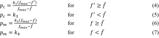
In this tool, adaptive crossover and mutation operators based on existing literature have been applied (Srinivas and Patnaik 1994). The adaptive crossover and mutation rates are implemented to allow the algorithm to self-tune and to correctly ensure that bad solutions have higher probability of changing. Similarly, this adaptive approach to these parameters allows the algorithm to better maintain a diverse population of the solution as the solution converges thereby allowing the GA to continue to operate effectively without terminating prematurely. These adaptive parameters are given by:

𝑝𝑐=𝑘1(𝑓𝑚𝑎𝑥−𝑓 ′₎

𝑓𝑚𝑎𝑥−𝑓̅ for 𝑓

′_{≥ 𝑓̅ (4)}

𝑝𝑐= 𝑘3 for 𝑓′< 𝑓̅ (5)

𝑝𝑚=𝑘2_𝑓(𝑓𝑚𝑎𝑥−𝑓)

𝑚𝑎𝑥−𝑓̅ for 𝑓 ≥ 𝑓̅ (6)

𝑝𝑚= 𝑘4 for 𝑓 < 𝑓̅ (7)

where 𝑝𝑐 is the probability of crossover, 𝑝𝑚 is the probability of

mutation, 𝑓𝑚𝑎𝑥 is the fitness of the best individual of the population, 𝑓′

is the fitness of the best parent, 𝑓̅ is the mean fitness value of the individuals in the population, and 𝑓 is the fitness of the individual under consideration. The constants are defined such that 𝑘1= 𝑘3= 1

and 𝑘2= 𝑘4=1₂.

Replacement. The final step of a steady-state GA procedure is to introduce the newly generated individuals into the next generation of the population. As an elitism parameter is used, the very best individuals within the population are carried over to the next generation and the remaining members of the population are replaced by the newly generated individuals. In this routine, a replace first weakest approach is taken. In this replacement strategy, child solutions are compared against the worst members in the current generation's population. If the child solution has a superior fitness value compared to the worst member of the population then the child is marked for inclusion in the next generation and the worst member is marked for removal. The process continues each time comparing the child's fitness against the worst member of the population that has not yet been marked for removal. In this specific case, an elitism parameter of 50% is used. The process, therefore, continues until 50% of the population has been replaced with new individuals.

This entire GA process is repeated until the solutions converges or the termination criteria are met.

For this study, a test case involving 30 turbines in a 47 km2 _{area was}

considered. For this area, bathymetry and seabed surveys were available defining the depth, areas where turbines cannot be placed, and areas where cables cannot be placed.

Table 2: GA Parameters

GA Encoding Discrete

Population Size 50 Maximum Generations 100 Probability of

crossover Adaptive

Probability of mutation Adaptive

Elitism 50%

Stop Criteria Loss of diversity or

maximum number of generations reached The GA was executed with a population size of 50. Previous work has found that for specific problem instances a smaller population size on the order of 20-30 individuals may work effectively (Haupt and Haupt 2004, Grefenstette 2006). For this problem, however, it was found that a smaller population size than 50 led to a loss in diversity after very few generations resulting in little improvement in the best individual before termination. Diversity in this case was defined as the proportion of the population which was unique solutions. A larger population size was therefore selected in order to ensure that diversity was maintained through the optimisation process.

For each proposed solution, the energy yield was first assessed, followed by execution of the intra-array cable optimiser after which the cost for the proposed layout was assessed. From this, the LCOE is evaluated assuming a constant capital expenditure (CAPEX) spend profile (50% each over 2 years), a 20 year project lifetime prior to decommissioning, and a discount rate of 8%.

A representative wind rose for a UK offshore site is assumed. This wind rose has strong winds principally from the south/south-west directions identifying this as the principle direction with which turbines should be aligned. This wind rose does not represent any site in particular, but is simply used for the demonstration of the capabilities of this tool.

positions aligned roughly perpendicular to the dominant wind direction. The grid generation algorithm removes positions on the grid which are in illegal positions (shown in grey in fig. 3). These illegal positions can be due to wrecks, UXOs, or the seabed slope. Each row of the grid is offset to ensure that the distance between turbines is increased along this dominant wind direction.

Fig. 2: Wind rose representing the wind resource for the test case.

Fig. 3: Generated grid of valid turbine positions from which turbine positions are selected.

RESULTS

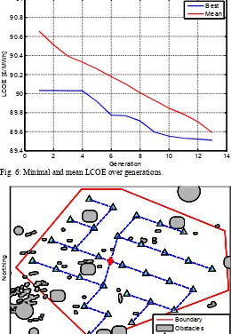
Executing the full approach for a wind farm containing 30 turbines resulted in the layout shown in fig. 4 after 13 generations. This solution was based on generating a grid made up of 50 potential turbine positions. This grid size was selected to ensure there were more possible turbine positions than turbines. The solution produced does adhere to the site constraints and produces a solution that conforms to a regular grid thereby satisfying the necessary navigational and search and rescue constraints. The solution produced also leaves larger gaps between turbines in the interior of the wind farm which is consistent with the relevant theory of wind turbine wakes and allows the wakes to recover before a new turbine is placed. Though significant gaps are left, the optimiser does not eliminate turbines from the centre of the wind farm. This indicates that AEP

could still be increased, but likely at a higher cost. The presence of the turbines in the centre of the wind farm indicates the importance of not only considering the wakes, but also the cost of the wind farm. Fig. 5 shows an inferior turbine layout proposed during the first generation of the optimisation process which has a higher LCOE of £92.45/MWh. As can be observed, fewer holes are left through the site, while a few turbines are isolated. The combined effect of this is that wake effects are not effectively minimised and costs are unnecessarily increased to accommodate the inclusion of the isolated turbines.

In this way, the approach ensures that all constraints are satisfied while at the same time using a dynamic spacing parameter to minimise the effect of wind turbine wakes and thereby the LCOE.

Fig. 4: Optimised turbine placement. LCOE for this layout is £89.51/MWh.

Fig. 5: An inferior layout proposed by the optimiser during the first generation. LCOE for this layout is £92.45/MWh.

From the convergence plot (fig. 6) it can be seen that over the execution of the algorithm, both the best and mean solution scores progressively improved. This is indicative that the GA was operating as expected. The final solution identified by the GA has an LCOE of 5%

10% 15%

20%

WEST EAST

SOUTH NORTH

0 - 5 5 - 10 10 - 15 15 - 20 20 - 25 25 - 30 5%

10% 15%

20%

WEST EAST

SOUTH NORTH

0 - 5 5 - 10 10 - 15 15 - 20 20 - 25 25 - 30

Easting

N

or

thi

ng

Boundary Obstacles

Valid Turbine Postions

Easting

N

or

thi

ng

Boundary Obstacles Turbines Substation Inter-Array Cables

Easting

N

or

thi

ng

£89.51/MWh.

Fig. 6: Minimal and mean LCOE over generations.

Fig. 7: The layout proposed by using DNV-GL WindFarmer’s Symmetrical Optimiser. LCOE for this layout is £90.53/MWh.

Running DNV GL WindFarmer’s Symmetrical Layout Optimisation as a benchmark on the same site yields a layout optimised for AEP (fig. 7). This layout which represents the industry standard approach to designing offshore wind farms produces a layout with an LCOE of £90.53/MWh when evaluated using our evaluation function. This is slightly higher than the solution produced by this tool, and broken down represents a 0.69% decrease in discounted AEP and a 0.44% increase in discounted cost compared to the solution generated by the GA shown in fig. 4. Though WindFarmer does not allow LCOE optimisation, it does represent the industry standard approach to designing wind farms. Further improvements to the proposed layout using the methodology at hand, could likely be found if the GA was run for more generations. Unfortunately, diversity was not maintained in the population and the optimiser was forced to stop prematurely. The scatter diagram in fig. 8 indicates the mean wind speed experienced by all turbines in each wind speed bin for different layouts relative to the mean free wind speed in each directional sector.

Using this approach for comparing the layouts, the relative wake loss by wind direction can be observed. From this figure, it can be observed that the inferior layout considered in fig. 5 leads to more significant reductions in the average wind speed in all wind directions than the more optimal layout shown in fig. 4. Though the relative decrease in wind speed is small, it is important to note that the power extracted by a wind turbine varies with the cube of the wind speed. This figure does also not consider the frequency of the wind directions, but is simply used to illustrate one of the key drivers of the LCOE. The overall wake loss is 4.39% for the inferior layout and 3.50% for the more optimal layout resulting in a change in AEP of 10,000 MWh per year.

Fig. 8: Scatter diagram showing the mean wind speed experienced through the wind farm for each direction sector for different layouts relative to the mean free wind speed in each direction.

DISCUSSION AND CONCLUSIONS

The present work has highlighted the initial results from the development of a framework for the optimisation of offshore wind farm layouts using an adaptive genetic algorithm. It is believed that this framework will be useful in furthering the field of offshore wind farm layout optimisation as well as allowing developers to better understand the characteristics of their potential projects. The approach taken has introduced as many realistic constraints as possible in order to maximise the value of the framework while at the same time striving for accurate assessment of the energy yield of the wind farm, the costs, and the LCOE.

For the test case considered, a 50 position discrete grid was generated prior to execution of the GA. This grid was oriented such that rows of turbines were perpendicular to the dominant wind direction. From this, the GA selected which 30 of the 50 positions should be used. Interestingly looking at the difference between the worst result of the first generation and the best result of the last generation, there is a difference of approximately £2/MWh indicating that significant savings can be reached by applying an optimisation algorithm rather than randomly selecting the positions. Comparing the results of the GA against the industry standard approach using DNV-GL WindFarmer also shows improvements in LCOE by optimising the layout considering LCOE using the GA rather than AEP using WindFarmer’s built in optimisation approach (£1/MWh improvement).

0 2 4 6 8 10 12 14

89.4 89.6 89.8 90 90.2 90.4 90.6 90.8 91

Generation

LC

O

E

[

£/

M

W

h

]

Best Mean

Easting

N

or

thi

ng

Boundary Obstacles Turbines Substation Inter-Array Cables

0 30 60 90 120 150 180 210 240 270 300 330

0.95 0.955 0.96 0.965 0.97 0.975 0.98 0.985 0.99 0.995 1

Wind Direction [°]

R

el

a

tiv

e

M

ea

n

W

in

d

S

pe

e

d

The number of valid turbine positions was selected arbitrarily to demonstrate the capabilities of this framework. Future work using this framework should explore the relationship between the number of turbines to be placed and the number of possible turbine positions in the discrete grid. Realistically, it would be expected that as the number of possible turbine positions increases, the solutions should improve in fitness however, at the same time as the number of possible positions increases, the regularity of the layout decreases and the search and rescue constraints will not remain satisfied. At the same time, the computational complexity will increase. With a grid including fewer holes than turbines, it was found that the search and rescue and navigational constraints were always satisfied, however, further work should explicitly explore this. Presently, the number of turbines to be positioned is also an input to the tool and further work should explore allowing the algorithm to select this as well with a maximum number of turbines constraint.

From the minimal and mean LCOE over generations plot (fig. 6) it can be seen that even though adaptive mutation and crossover rates are used, the GA still has some generations where though the population overall improves, the best solution does not. This indicates that further work could explore tuning of the GA parameters to improve the number of generations it takes to converge. Presently, however, the GA is terminating due to a loss in diversity, rather than true convergence, and improvements can be expected if methods for maintaining diversity in the population are introduced to the GA. Having said that, even without any further tuning, the GA still manages to identify a layout with a lower LCOE than using the industry standard approach with DNV-GL WindFarmer. This highlights the need to not only optimise for a metric taking into account both energy yield and cost, but also the advantage of introducing holes to a regular layout.

Given this platform, future work will expand on this study and look not only at further tuning the GA parameters to effectively solve this problem, but also to benchmark the GA against alternate optimisation algorithms. This platform will also allow alternate objective functions such as levelised production cost (LPC) or net present value (NPV) to be explored.

Application of this framework will also allow simplifications of the evaluation function to be explored. Presently, the evaluation function is relatively detailed with the majority of time being spent on evaluating the intra-array cable infrastructure and optimising this for each turbine layout under consideration. Having said this, each evaluation call on an 8 core computer is still completed in under a minute. Future work using this framework will also be capable of comparing the results using alternate evaluation functions and characterising which elements of the layout the objective function is most sensitive to. At the same time, however, it is believed that the tool can scale to larger problems representing realistic offshore wind farms without an unrealistic increase in the computational power required. One iteration of 50 individuals has been run on a multi-cored desktop machine, however, it is expected that for a full-sized wind farm the execution of the tool will be transferred to a cluster allowing the larger problem to be solved in similar timescales as the test case by utilising more cores in parallel. Moving away from a single processor will also allow larger population sizes to be explored potentially allowing the premature convergence problems to be avoided. Realistically for a full wind farm it would be expected that in lieu of using an extremely large population, multiple runs will be completed using slightly larger populations with random seeding in order to

ensure that the search space is effectively explored.

The applicability of this tool to larger offshore wind farms is still limited due to the simplification of the wakes, and the omission of the interactions between wind turbines and the atmospheric boundary layer (Frandsen et al. 2006). This large wind farm or deep-array effect has been explored by adding corrections to analytic wake models (Barthelmie et al. 2007, Brower and Robinson 2009). Future work intends on using the constructed framework to validate and tune these correction factors before applying them in the overall layout optimisation approach.

ACKNOWLEDGEMENTS

This work is funded in part by the ETI and RCUK Energy programme for IDCORE (EP/J500847/1).

REFERENCES

Ainslie, J., 1988. Calculating the flowfield in the wake of wind turbines. Journal of Wind Engineering and Industrial Aerodynamics, 27, 213–224.

Anderson, M., 2009. Simplified Solution to the Eddy-Viscosity Wake Model.

Arthur, D. and Vassilvitskii, S., 2006. k-means ++ : The Advantages of Careful Seeding. Proceedings of the eighteenth annual ACM-SIAM symposium on Discrete Algorithms, 8, 1–11.

Barthelmie, R.J., Folkerts, L., Larsen, G.C., Frandsen, S.T., Rados, K., Pryor, S.C., Lange, B., and Schepers, G., 2006. Comparison of Wake Model Simulations with Offshore Wind Turbine Wake Profiles Measured by Sodar. Journal of Atmospheric and Oceanic Technology, 23 (7), 888–901.

Barthelmie, R.J., Hansen, K., Frandsen, S.T., Rathmann, O., Schepers, J.G., Schlez, W., Phillips, J., Rados, K., Zervos, A., Politis, E.S., and Chaviaropoulos, P.K., 2009. Modelling and Measuring Flow and Wind Turbine Wakes in Large Wind Farms Offshore. Wind Energy, 12 (June), 431–444.

Barthelmie, R.J., Rathmann, O., Frandsen, S.T., Hansen, K.S., Politis, E., Prospathopoulos, J., Rados, K., Cabezón, D., Schlez, W., Phillips, J., Neubert, a, Schepers, J.G., and Pijl, S.P. Van Der, 2007. Modelling and measurements of wakes in large wind farms. Journal of Physics: Conference Series, 75, 012049. Brower, M. and Robinson, N., 2009. The openWind deep-array wake

model: development and validation.

Burton, T., Jenkins, N., Sharpe, D., and Bossanyi, E., 2011. Wind energy handbook. Second. John Wiley & Sons, Ltd.

Crasto, G. and Castellani, F., 2013. Wakes Calculation in a Offshore Wind Farm. Wind Engineering, 37 (3), 269–280.

DNV GL - Energy, 2014. WindFarmer Theory Manual. Elkinton, C.N., 2007. Offshore Wind Farm Layout Optimization.

University of Massachussetts Amherst.

Fagerfjäll, P., 2010. Optimizing wind farm layout – more bang for the buck using mixed integer linear programming. Chalmers University of Technology and Gothenburgh University. Frandsen, S., Barthelmie, R., and Pryor, S., 2006. Analytical

modelling of wind speed deficit in large offshore wind farms.

Wind Energy, (January), 39–53.

Gaumond, M., Rethore, P., and Bechmann, A., 2012. Benchmarking of Wind Turbine Wake Models in Large Offshore Windfarms.

Proceedings of the Science of Making Torque from Wind Conference.

(2), 259–270.

Grefenstette, J.J., 2006. Optimization of Control Parameters for Genetic Algorithms. IEEE Transactions on Systems, Man, and Cybernetics, SMC-16 (February), 122–128.

Guillen, F.B., 2010. Development of a design tool for offshore wind farm layout optimization. Delft University of Technology. Haupt, R.L. and Haupt, S.E., 2004. Practical Genetic Algorithms.

Second. Wiley-Interscience Publication.

Holland, J.H., 1992. Adaptation In Natural And Artificial Systems. [Electronic Resource] : An Introductory Analysis With Applications To Biology, Control, And Artificial Intelligence. Second. Cambridge, Mass.: MIT Press.

Ishihara, T., Yamaguchi, a., and Fujino, Y., 2004. Development of a new wake model based on a wind tunnel experiment. Global Wind Power, 6.

Katic, I., Højstrup, J., and Jensen, N.O., 1986. A Simple Model for Cluster Efficiency. European Wind Energy Conference and Exhibition 1986, (October), 407–410.

Larsen, G.C., 1988. A Simple Wake Calculation Procedure. Larsen, G.C., Madsen, H.A., Troldborg, N., Larsen, T.J., Réthoré,

P.-E., Fuglsang, P., Ott, S., Mann, J., Buhl, T., Nielsen, M., Markou, H., Sørensen, J.N., Hansen, K.S., Mikkelsen, R., Okulov, V., Shen, W.Z., Heath, M., King, J., McCann, G., Schlez, W., Carlén, I., Ganander, H., Migoya, E., Crespo, A., Jiménez, A., Prieto, J.L., Stidworthy, A., Carruthers, D., Hunt, J., Gray, S., Veldkamp, D., Mouritzen, A.S., Jensen, L., Krogh, T., Schmidt, B., Argyriadis, K., and Frohnböse, P., 2011.

TOPFARM - Next Generation Desgin Tool for Optimisation of Wind Farm Topology and Operation. Roskilde, Denmark: Information Service Department, Risø National Laboratory for Sustainable Energy Technical University of Denmark. Larsen, G.C. and Réthoré, P.E., 2013. TOPFARM - A Tool For Wind

Farm Optimization.

MacQueen, J., 1967. Some methods for classification and analysis of multivariate observations. Proceedings of the fifth Berkeley symposium on Mathematical Statistics and Probability, 233 (233), 281–297.

Mosetti, G., Poloni, C., and Diviacco, B., 1994. Optimization of wind turbine positioning in large wind-farms by means of a genetic algorithm. Journal of Wind Engineering and Industrial Aerodynamics, 51 (1), 105–116.

NOREL Group, 2013. Nautical and Offshore Renewable Energy Liaison Group (NOREL) Action Points from the 27th NOREL held on 11 July 2013.

Pérez, B., Mínguez, R., and Guanche, R., 2013. Offshore wind farm layout optimization using mathematical programming techniques. Renewable Energy, 53, 389–399.

Pillai, A.C., Chick, J., Johanning, L., Khorasanchi, M., and de Laleu, V., 2015. Offshore wind farm electrical cable layout

optimization. Engineering Optimization, 47 (12), 1689–1708. Pillai, A.C., Chick, J., and de Laleu, V., 2014. Modelling Wind

Turbine Wakes at Middelgrunden Wind Farm. In: Proceedings of EWEA 2014.

Renkema, D.J., 2007. Validation of wind turbine wake models. TU Delft.

Sanderse, B., Pijl, S., and Koren, B., 2011. Review of computational fluid dynamics for wind turbine wake aerodynamics. Wind Energy, (February), 799–819.

Schlez, W. and Neubert, A., 2009. New developments in large wind farm modelling. Proceedings of EWEC 2009.