The anchorage-slip effect on direct displacement-based design of R/C bridge piers for limiting material strains

City, University of London Institutional Repository

Citation

:

This is the accepted version of the paper.

This version of the publication may differ from the final published

version.

Permanent repository link:

Link to published version

:

Copyright and reuse:

City Research Online aims to make research

outputs of City, University of London available to a wider audience.

Copyright and Moral Rights remain with the author(s) and/or copyright

holders. URLs from City Research Online may be freely distributed and

linked to.

The anchorage-slip effect on direct displacement-based

design of R/C bridge piers for limiting material strains

P.E. Mergos*1

1_{Technological Educational Institute of Chalkida, Chalkida 34400, Greece}

Abstract: Direct displacement-based design (DDBD) represents an innovative philosophy for seismic design of structures. When structural considerations are more critical, DDBD design should be carried on the basis of limiting material strains since structural damage is always strain related. In this case, the outcome of DDBD is strongly influenced by the displacement demand of the structural element for the target limit strains. Experimental studies have shown that anchorage slip may contribute significantly to the total displacement capacity of R/C column elements. However, in the previous studies, anchorage slip effect is either ignored or lumped into flexural deformations by applying the equivalent strain penetration length. In the light of the above, an attempt is made in this paper to include explicitly anchorage slip effect in DDBD of R/C column elements. For this purpose, a new computer program named RCCOLA-DBD is developed for the DDBD of single R/C elements for limiting material strains. By applying this program, more than 300 parametric designs are conducted to investigate the influence of anchorage slip effect as well as of numerous other parameters on the seismic design of R/C members according to this methodology.

Keywords: seismic design; reinforced concrete; displacement-based; anchorage slip;

material strains.

1. Introduction

Current code provisions implement force-based procedures for seismic design of R/C structures. However, force-based design is against physical reality (Fardis 2009). It is known that damage is directly related to member deformations or lateral drifts (Priestley et al. 2007). Hence, displacement-based design represents a more rational approach for structural design against seismic demand.

A number of displacement-based methodologies have been developed for seismic design (fib Task Group 7.2, 2003). One of the best-known procedures that falls within this category is the Direct Displacement Based Design (DDBD), which was initially developed by Priestley (1993) and Priestley and Kowalsky (2000). This approach, which connects directly the level of structural damage to the design strength, is well documented (Priestley 2003, Priestley et al. 2007), it is relatively easy to apply and well suited to incorporation in design codes (Calvi and Sullivan 2009).

hinge regions to achieve the design goals in terms of pre-defined deformations or displacements (Priestley 2003).

For DDBD, the performance limit state may be defined by either limiting material strains or lateral drifts. The former is the case when structural considerations are more critical since damage is strain-related for structural elements. The latter occurs when non-structural considerations control the design since damage to non-structural elements can be generally considered as drift-related (Priestley 2007).

When designing an R/C column element according to DDBD for limiting concrete or steel strains, the design strength depends on the displacement demand of the member for these material strains. Since the displacement demand depends is influenced by the reinforcement content of its critical cross-section, an iterative procedure is generally required. Hence, the design process may become considerably time-consuming.

In this study, a new computer program, named RCCOLA-DBD, is developed, which automates, for the first time, the aforementioned design procedure for single R/C column members. By applying this design tool, the required design effort is minimized, while maximum accuracy is assured.

Furthermore, several experimental studies have shown that fixed end rotations caused by anchorage slip effect contribute significantly (up to 50%) to the total displacement capacity of an R/C member (Ma et al. 1976, Saatcioglu and Ozcebe 1989, Lehman and Moehle 1998). Since this displacement capacity represents the design displacement for DDBD for limiting deformations, it is evident that anchorage slip may play a vital role on the determination of the required design strength. Nevertheless, in all applications of DDBD until this moment, anchorage slip effect is either ignored or lumped into flexural deformations by applying the equivalent strain penetration length. As it will be shown later in this paper, this simplifying procedure may lead, in some cases, to erroneous results because it is not able to capture several aspects of the anchorage slip phenomenon. To resolve this controversy, it is proposed in this paper that anchorage slip effect is considered explicitly in the analytical procedure.

In the following, the procedure for determination of the force-displacement response of R/C members accounting explicitly for anchorage slip effect is described. Then, the methodology of DDBD for limiting material strains is outlined as well as its implementation in RCCOLA-DBD. Finally, more than 300 parametric designs are performed in order to investigate the influence of anchorage slip effect, as well as of numerous other design parameters, on the analytical results of DDBD of single R/C members for limiting material strains.

2. Force-displacement response of R/C members accounting explicitly for anchorage slip effect

One of the basic prerequisites of DDBD for limiting material strains is the derivation of the force-lateral displacement response of the R/C member under investigation. It is known that the total lateral tip displacement of an R/C cantilever can be considered as the sum of the displacements caused by flexural and shear deformations along its length as well as the displacement caused by the fixed-end rotation developed at its base due to anchorage slip effect.

to DDBD for limiting strains, since this reduces the displacement demand of the R/C member. For this reason, in the following, shear displacement is ignored. However, it is important to state that for the other R/C members shear deformations and shear-flexure interaction effect (Mergos and Kappos 2008, 2010, Beyer et al. 2011), should be taken into consideration in the design procedure.

Figure 1: Lateral deformation of an R/C cantilever: a) R/C member; b) SDOF representation; c) moment diagram; d) displacement profile

Fig. 1 presents an R/C column cantilever as well as its SDOF representation. The most realistic structure conforming to the assumptions of a SDOF approximation is a regular bridge under transverse excitation. The height and effective mass of the cantilever are H and meff respectively. The cantilever is subjected to a lateral force F

causing a bending moment M=F·H at its base.

The first step to define the displacement response of the R/C member is to perform a moment-curvature analysis of its critical cross-section. For this purpose, RCCOLA-DBD uses the well known program RCCOLA developed initially by Mahin and Bertero (1977) at UC Berkeley and later modified by Kappos (2002). For a given cross section, reinforcement, axial load N and strain at the extreme compression fibre εc the corresponding bending moment M and curvature φ are determined by applying

an iterative procedure for the neutral axis depth c. This procedure is repeated for increasing levels of εc and the complete M-φ envelope curve of the cross-section

under examination is determined for the given level of axial load.

Several constitutive material laws have been implemented in RCCOLA for the confined and unconfined concrete and the reinforcing steel under monotonic loading. In the following, the Kappos (1991) model for confined concrete and the Park and Sampson (1972) material law for reinforcing steel are assigned.

The strain limits for M-φ analysis depend on the design limit state. For the damage control limit state the limit to confined concrete compression strain εcu is usually

taken to occur when fracture of the transverse reinforcement confining the core takes place. For this state, the Mander et al. (1986) criterion is adopted herein given by Eq. (1), where ρw, fyw and εsw,ult are the volumetric ratio, yield strength and strain at

maximum strength of the transverse reinforcementand fcc is the maximum strength of

the confined concrete. The limit to the extreme tension reinforcement strain may be taken as a predefined value (e.g. 0.05) or as a fraction of the strain at maximum stress εsu (e.g. 0.6εsu). Apparently, the ultimate curvature φu and moment Mu capacity are

determined by the minimum values corresponding to one of these strain limits.

,

0.004 1.4 ρw fyw εsw ult

ε = + ⋅ ⋅ ⋅ (1)

F

H

meff

M=F·H

∆fl

∆sl

a) b) c) d)

M

θsl My

Mu

Bilinear

Analytical

θy,sl θu,sl

For design purposes, it is generally sufficient to adopt a bilinear approximation of the actual M-φ response (Fig. 2a). In this study, the respective methodology described analytically in Priestley et al. (2007) is adopted. Following this analytical procedure, the equivalent yielding moment My and curvature φy are determined.

It is known that the calculation of the top displacement response of an R/C cantilever by integrating the curvature profile derived by the moment diagram and the M-φ analysis described in the preceding paragraphs does not agree with the experimental observations. This is due to the tension shift, anchorage slip and shear deformation effects.

To overcome these difficulties, typically, the concept of the equivalent plastic hinge length Lp is adopted (Pauley and Priestley 1992), over which the curvature is assumed

to be constant and equal to the respective value at the cantilever base. The curvature distribution outside this length is assumed to be linear. This compensates for tension shift effect and partially for shear deformations (Priestley et al. 2007).

The plastic hinge length incorporates the strain penetration length Lsp, which aims at

accounting for the fixed end rotation caused by anchorage slip effect. Hence, Lp is

given by Eq. (2), where k factor accounts for strain hardening effect.

2

p sp sp

L = ⋅k H+L ≥ ⋅L (2)

Various relationships (fib Chapter 4) can be found in the literature for k and Lsp.

Herein, the proposals by Priestley et al. (2007) are adopted, as shown in the following equations, where fyl, ful and dbl are the yield and ultimate strength and bar diameter of

the longitudinal reinforcement.

0.022

sp yl bl

L = ⋅f ⋅d (3)

0.2 ul 1 0.08

yl

f k

f

 

= ⋅_ − _≤

  (4)

Figure 2: Bilinear approximations: a) moment-curvature; b) moment-anchorage slip rotation envelopes

Following the concept of the plastic hinge length, the cantilever tip displacements at yielding ∆y and ultimate ∆u states are given by Eqs (5) and (6) respectively.

(

)

/ 3

y ϕy H Lsp

∆ = ⋅ + (5)

(

)

u y ϕu ϕy Lp

∆ = ∆ + − ⋅ (6) It can be inferred from the above that the fixed end rotations caused by anchorage slip

effect are taken indirectly into account in the calculations by the empirical strain penetration length Lsp and the results of M-φ analysis of the critical cross section.

M

φ

My Mu

Bilinear

Analytical

φy φu

However, as it will be shown later on, in this way various parameters affecting anchorage slip like bond strength, hardening of the reinforcing steel, anchorage detailing cannot be captured with sufficient accuracy. This issue becomes more important for DDBD for limiting material strains, since fixed end rotations may influence significantly the displacement demand of the R/C member for these material strains and consequently the design strength of its critical cross section.

For this reason, it is proposed herein that anchorage slip is included explicitly in the design procedure. Various analytical methodologies have been developed so far for the determination of fixed-end rotations caused by anchorage slip effect (Otani and Sozen 1972, Filippou 1985, Alsiwat and Saatcioglu 1992, Lowes and Altoontash 2003, Sezen and Setzler 2008). Herein, the Alsiwat and Saatcioglu (1992) analytical procedure is adopted, which has been proven to provide adequate correlation with the experimental evidence, while it remains simple enough in order to be easily incorporated in seismic design of R/C members.

According to this methodology, the moment-anchorage slip rotation (M-θsl)skeleton

curve is derived on the basis of assuming uniform bond stress distribution along different segments of the anchored rebar (Fig. 3d). These segments are the elastic region Le, the strain-hardening region Lsh and the pullout cone region Lpc. Following

the experimental observations of Lehman and Moehle (1998) regarding well confined concrete bridge columns, the average bond strength τbe is taken here equal to 1.0√fc

for the elastic region and the bond resistance τbf corresponding to Lsh equal to 0.5√fc.

The same values have been assigned by Sezen and Setzler (2008) providing adequate match with the experimental recordings. In the pullout cone region, it is assumed that the acting bond is negligible.

For various levels of the applied end moment and using the results of M-φ analysis, the stress σs and strain εs of the reinforcing bar at the loaded end are first determined.

Then, from equilibrium and applying the assumed bond distribution, variation of reinforcing bar stress σs(x) along the embedment length is defined as shown in Fig.

3b, where σy is the yield strength of steel and σh is the stress at the end of the straight

part of the rebar anchorage. Then, by assigning an appropriate constitutive material law for steel (Park and Sampson 1972), strain distribution εs(x) is determined, as

shown in Fig. 3c, where εy and εsh are the steel strains at the onset of yielding and

strain hardening, respectively, and εh is the steel strain at the end of the straight part of

the anchorage. It is important to note that post-yield nonlinearity of the material constitutive law, i.e. strain hardening, should be taken into account because it affects significantly the final results (Mergos 2011, 2012).

Once εs(x) is determined, slip of the reinforcement δslip can be calculated by

integration along the anchorage length of the bar. In the case of hooked bars, local slip of the hook should be added. This can be evaluated by the force acting on the hook Ph=Ab·σh, where Ab is the area of the anchored bar, and an appropriate hook force vs.

hook slip relationship (Soroushian et al. 1988).

Upon determination of δslip, the respective fixed-end rotation can be calculated by Eq.

(7), where (d-xc) is the distance between the bar and the neutral axis. The envelope

M-θsl curve constructed by the various points of the afore-described methodology is then

idealized by a bilinear relationship for the purposes of analysis (Fig. 2b). It is noted that since the reinforcement anchorage is designed to avoid brittle pullout failure, it can be assumed that the failure point (θu,sl, Mu) of the bilinear M-θsl curve corresponds

to the ultimate point of the bilinear M-φ curve (φu, Mu). For reasons of simplicity, it is

respective method of the M-φ envelope curve. This effectively means that both bilinear envelopes yield at the same equivalent yielding moment My (Fig. 2).

slip sl

c

d x δ θ =

− (7)

Figure 3: a) Reinforcing bar with 90o _{hook embedded in concrete; b) steel stress distribution;}

c) strain distribution; d) bond stress distribution.

By modelling explicitly fixed end rotations caused by anchorage slip, the cantilever tip displacements at yielding ∆y and ultimate ∆u states are now given by Eqs (8) and

(9) respectively.

2 ,

/ 3

y ϕy H θy sl H

∆ = ⋅ + ⋅ (8)

(

)

(

)

, ,

1 / 2 ( )

u y ϕu ϕy k k H θu sl θy sl H

∆ = ∆ + − ⋅ ⋅ − ⋅ + − ⋅ (9)

3. Direct displacement-based design for limiting material strains formulation

The vertical R/C cantilever structure of Fig. 1a is represented by the SDOF system of Fig. 1b. The bilinear envelope of the lateral force-displacement response of the SDOF representation is shown in Fig. 4a, where an initial stiffness Kis followed by a post yield stiffness r·K.

DDBD characterizes the structure by secant stiffness Ke at maximum displacement ∆d

and a level of equivalent viscous damping ξeq representative of the combined elastic

damping and the hysteretic energy absorbed during inelastic response (Priestley 2003).

The first step of DDBD for limiting concrete and steel strains εcd and εsd is the

computation of the yield ∆y and design displacement ∆d for these strain limits. This

can be achieved by Eqs (5,6,8,9) by setting φu and θu,sl equal to the design curvature

φd and fixed-end rotation θd,sl corresponding to the most critical strain among εcd and

εsd.

σs

εs

εs

Lpc

σs(x)

εy

τbe

Lsh

Lstraight

c) b) a)

Le

σh

εh

εs(x)

σy

x

τbf

F

∆

Fy Fu

∆y ∆d

K

r·K

Ke

∆

T

∆d

Te Tc

ξeq

5%

∆c,5

a) b)

Nevertheless, it is evident from these equations that for calculation of ∆y and ∆d the

reinforcement configuration should be predefined. Hence, in general, an iterative procedure is required, which may increase considerably the computational effort. In this study, this procedure is automated by developing the computer program RCCOLA-DBD as described in the following.

The equivalent viscous damping ξeq is determined as a function of the displacement

ductility demand µd= ∆d/∆y. Different equations have been proposed (Grant et al.

2005, Dwairi et al 2007) for estimating ξeq by µd depending on the structural type.

Herein, the following equation is applied, as proposed by Dwairi et al. (2007) for concrete wall buildings and bridges.

1 0.05 0.444 d eq

d

µ ξ

π µ

 − 

= + _{⋅ }

⋅

  (10)

Figure 4: a) Effective stiffness Ke of the equivalent SDOF system at peak response; b) design

displacement spectra.

With the design displacement ∆d determined and the corresponding ξeq damping

estimated from µd, the effective period Te at maximum response can be read from a

set of displacement spectra for different levels of damping, as shown in Fig. 4b. In this figure, a typical design displacement spectra set for damping levels 5% and ξeq is

presented. Displacements for the 5% spectrum increase with period up to a value ∆c,5

corresponding to the corner period Tc. For normal accelerograms measured at least

10km from the fault rupture, the displacements ∆Τ,ξ corresponding to a different level

of damping ξeq can be related to the displacements for 5% damping ∆Τ,5 by the EC8

expression:

0.5 , ,5

0.10 0.05

T T

eq

ξ _ξ

 

∆ = ∆ ⋅_ _

+

  (11)

In the following, the small nonlinearity at low periods of the displacement spectra is ignored since it is unlikely to be significant for displacement-based designs, where the effective period at maximum response is typically very high (Priestley 2003). By this assumption, for the design displacement ∆d and equivalent damping ξeq, the effective

period Te is calculated by the respective displacement spectrum (Fig. 4b) as

0.5

,5

0.05 0.10

eq d

e c

c

T =T ⋅ ∆ ⋅  +ξ _

∆ _{ } (12)

2

2 2

,5

2 2 2

4 4 0.10

0.05

c

e e

e

e c d eq

m m

K

T T

π π

ξ

 

∆

⋅ ⋅ ⋅ ⋅

= = ⋅ ⋅_ _

∆ _ + _ (13)

Finally, the design base shear VB is determined as

2 2

,5 2

4 0.10

0.05

c e B e d

c d eq

m

V K

T π

ξ

 

∆

⋅ ⋅

= ⋅ ∆ = ⋅ ⋅_ _

∆ _ + _ (14)

Upon determination of VB, the design moment of the critical cross-section

Mdem=VB·H is defined. Then, the longitudinal reinforcement of this section is

determined in order to yield this moment capacity for the given level of axial load and the critical limiting material strain εcd or εsd.

The transverse reinforcement may be given a predefined configuration for construction reasons but in any case it should be adequate to assure the design concrete limiting material strain εcd as determined by Eq. (1). For this calculation, a

short iterative procedure is required since the confined concrete strength fcc is also a

function of the transverse reinforcement volumetric ratio ρw.

In some cases, the procedure described above may require considerable computational effort since the displacement demand ∆d and consequently the design shear VB of the

R/C member depends on its reinforcement content. Nevertheless, effective design tools have not yet been developed to simplify this methodology.

In this study, this design methodology is automated by developing the computer software RCCOLA-DBD. RCCOLA-DBD utilizes the well-known program RCCOLA (Mahin and Bertero 1977) for the M-φ analysis of the critical cross-section of the R/C cantilever under examination. An additional subroutine has been introduced in RCCOLA by the writer of this paper (Mergos 2011) to perform the M-θsl analysis, following the procedure (Alsiwat and Saatcioglu 1992) described in the

preceding section. Furthermore, additional lines have been written for the bilinearization of the analytical M-φ and M-θsl envelopes according to the Priestley et

al. (2007) methodology.

The flowchart of RCCOLA-DBD is presented in Fig. 5. Required data are the R/C cantilever geometry, material properties, limiting material strains, design displacement spectra, reinforcing bars distribution, anchorage detailing, maximum ρmax and minimum ρmin allowable volumetric ratios of the critical section longitudinal

reinforcement and the allowable design moment tolerance tol. The outcomes of RCCOLA-DBD are the required longitudinal ρl and transversal ρw reinforcement

volumetric ratios. As it can be seen in Fig. 5, RCCOLA-DBD employs the interval bisection root solution algorithm for the determination of ρl. Depending on the

comparisons between moment demand Mdem and moment capacity Mcap, the program

narrows the ρl solution limits until convergence between Mdem and Mcap is achieved

Figure 5: RCCOLA-DBD flowchart

Read input data and limiting material strains εcd and εsd

Determine ρw to fulfill Eq. (1) for εcd

Update counter I=I+1

Call RCCOLA to determine Μ-φ and Μ-θsl envelopes and their

bilinear approximations. Determination of the moment capacity Mcap corresponding to the critical material strain εcd or εsd

Determination of ∆y, ∆d, ξeq, VB from RCCOLA output and

Eqs. (8), (9), (10), (14) respectively.

Calculation of the moment demand: Μdem=VB·H

Assumption for ρl:

if I=1 then ρl=ρmin

if I=2 then ρl=ρmax

if Ι>2 then ρl=(ρmin+ ρmax)/2

Is Ι=1 and Μdem<(1-tol)·Mcap ?

END

YES

(required ρl<ρmin)

NO

Further iteration is required

Is I=2 and Μdem>(1+tol)·Mcap ?

Is abs((Μdem/Mcap)-1)<tol ?

if Μdem<Mcap then set ρmax=ρl

if Μdem>Mcap then set ρmin=ρl

YES

(design completed)

YES

(required ρl>ρmax)

Design not feasible

4. Design applications

4.1 Basic design example

In this section, the basic design example is described. This case study is used as reference, in the next section, for numerous parametric designs aiming at illustrating the influence of various parameters on the outcome of DDBD for limiting material strains.

The basic case study is shown in Fig. 6. It is an R/C bridge pier with a 1.0m square or circular cross-section. The longitudinal reinforcement is assumed evenly distributed around the perimeter. The cover to flexural reinforcement is taken 50mm. The height of the cantilever is H=5.0m. The yield strength fyl, strain hardening ful/fyl, strain at

maximum strength εsu and bar diameter dbl of the longitudinal reinforcement are

500MPa, 1.35, 0.15 and 20mm respectively. The yield strength and strain at maximum strength εsw,ult of the transverse reinforcement are also assumed 500MPa

and 0.15. Concrete strength fc is 30MPa and the anchorage is assumed to be straight

(without end-hook).

For both sections to yield similar results, it is assumed that the axial load ratios of the square and the circular cross-sections are 0.13 and 0.10 respectively. The corner period Tc and displacement ∆c,5 of the 5% displacement spectrum are taken as 4.0sec

and 0.6m. Finally, the limiting material strains for concrete εcd and steel εsd are taken

equal to 0.015 and 0.05 respectively.

Figure 6: Basic design case study: a) R/C bridge pier; b) SDOF representation; c) square cross-section; d) circular cross-section

Table 1 summarizes the iterative design procedure performed by RCCOLA-DBD for the basic design example and the circular cross-section. The Mdem/Mcap ratio tolerance

is specified equal to 1%. The ρl limits ρmin and ρmax are set initially equal to 0.2% and

8%. Of course, these limits are not allowed for construction reasons, but they are chosen herein to cover all possible parametric designs of the following section. Convergence is achieved after 8 iterations. It is worth noting that the 4th iteration is very close to convergence (error approximately 3%), but in order to fulfill the strict pre-specified tolerance (1%) further iterations are necessary. If narrower ρl limits

were chosen, the convergence would be faster. The final required longitudinal reinforcement volumetric ratio is calculated as 2.03%. The necessary transverse reinforcement ratio to achieve εcd=0.015 is ρw=0.34%.

F

H

meff

a) b) c)

N

1.0m

1.

0m

1.

0m

Similar calculations for the square cross-section yield that the required longitudinal reinforcement is ρl=2.27%.

Table 1: Iterative design procedure for the basic design example and the circular cross-section

Iteration

Parameter 1 2 3 4 5 6 7 8

ρmin (%) 0.2 0.2 0.2 0.2 0.2 1.175 1.663 1.906

ρmax (%) 8.0 8.0 8.0 4.1 2.15 2.15 2.15 2.15

ρl (%) 0.2 8.0 4.1 2.15 1.175 1.663 1.906 2.028

φy (rad/m) 0.0046 0.0061 0.0060 0.0057 0.0054 0.0055 0.0056 0.0056

θy,sl (rad) 0.00098 0.00114 0.00125 0.00119 0.00113 0.00116 0.00118 0.00118

φd (rad/m) 0.0675 0.0361 0.0407 0.0467 0.0534 0.0494 0.0479 0.0473

θsl,d (rad) 0.0110 0.00409 0.00496 0.00626 0.00774 0.00684 0.00652 0.00638

∆y (m) 0.043 0.057 0.056 0.053 0.050 0.052 0.053 0.053

∆d (m) 0.200 0.122 0.133 0.148 0.164 0.154 0.151 0.149

µ∆ 4.608 2.148 2.376 2.776 3.271 2.970 2.864 2.819

ξeq 0.161 0.126 0.132 0.140 0.148 0.144 0.142 0.141

Te (sec) 1.935 1.079 1.198 1.361 1.542 1.433 1.393 1.376

VB (kN) 496.01 974.61 862.40 741.77 641.60 698.52 721.70 732.28

Mdem (kNm) 2480.07 4873.08 4312.01 3708.85 3208.02 3492.61 3608.50 3661.42

Mcap (kNm) 1255.59 10592.4 6144.71 3828.90 2600.65 3223.87 3527.63 3680.32

Mdem/Mcap 1.975 0.460 0.702 0.969 1.234 1.083 1.023 0.995

4.2Parametric designs

In this section, parametric designs are conducted according to the DDBD for limiting material strains methodology and by the application of RCCOLA-DBD. The design example of the previous section serves as the basis for this parametric study. In each case, one design parameter of this example is modified in order to investigate its effect on the final outcome of DDBD.

In addition, to examine the influence of anchorage slip effect, three different models are applied in the analytical procedure. The A model considers only flexural deformations in the calculation of ∆y and ∆d. Hence, anchorage slip effect is totally

disregarded for this model. The B model (proposed model) takes explicitly anchorage slip effect through the procedure described previously in this study. Finally, C model accounts for anchorage slip effect by the application of Eq. (2) for the plastic hinge length, as proposed by Priestley et al. (2007).

It is important to note that in all cases, Teff remains always lesser than Tc (hence Eq.

14 always holds) and the lateral drift limit does not exceed 0.045. The analytical results of the parametric study are presented in the following.

4.2.1 The limiting concrete strain εcd

Herein, the variation of longitudinal reinforcement demand is examined with the limiting concrete strain εcd. For this reason, the basic design example is solved for six

different values of εcd=0.009, 0.012, 0.015, 0.018, 0.021 and 0.024. The required ρw to

achieve these strains are 0.15%, 0.24%, 0.34%, 0.44%, 0.54% and 0.65% respectively. However, ρw was not taken lesser than 0.22% and 0.30% for the circular

and the rectangular cross-section respectively corresponding to single stirrups

ø

decreases. This is rational since smaller εcd means less damage for the R/C member. It

0.024. This is because, for these models and concrete strains, the steel limiting strain εsd=0.05 becomes more critical than εcd.

Furthermore, from the comparisons of the results of models A, B and C, it is concluded that anchorage slip effect plays a vital role on the determination of ρl. In

some cases, model A, which ignores anchorage slip effect, yields up to 3 times more longitudinal reinforcement demand than model C. Models B and C tend to coincide as εcd increases, but they provide considerably different predictions for small values of

εcd. For these design examples, model B yields safer designs than model C.

Fig. 7: Variation of the longitudinal reinforcement demand with the limiting concrete strain εcd for the a) circular; b) square cross-section.

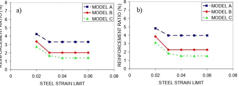
4.2.2 The limiting steel strain εsd

Herein, the variation of longitudinal reinforcement demand is examined with the limiting steel strain εsd. For this reason, the basic design example is solved for five

different values of εsd=0.02, 0.03, 0.04, 0.05 and 0.06. It can be seen that ρl demand

decreases as εsd increases. This is expected since more damage is accepted in this

manner. However, when εsd becomes higher than 0.03 for models A and B and 0.04

for model C, ρl demand remains constant since concrete limiting strain εcd=0.015 is

more critical in these cases.

Fig. 8: Variation of the longitudinal reinforcement demand with the limiting steel strain εsd for

the a) circular; b) square cross-section.

0 1 2 3 4 5 6 7 8

0 0.005 0.01 0.015 0.02 0.025 0.03 CONCRETE STRAIN LIMIT

R E IN F O R C E M E N T R A T IO ( %

) _{MODEL A}

MODEL B MODEL C 0 1 2 3 4 5 6 7 8

0 0.02 0.04 0.06 0.08 STEEL STRAIN LIMIT

R E IN F O R C E M E N T R A T IO ( %

) _{MODEL A}

MODEL B MODEL C a) 0 1 2 3 4 5 6 7 8

0 0.005 0.01 0.015 0.02 0.025 0.03 CONCRETE STRAIN LIMIT

R E IN F O R C E M E N T R A T IO ( %

) _{MODEL A}

MODEL B MODEL C b)

a) b)

0 1 2 3 4 5 6 7 8

0 0.02 0.04 0.06 0.08 STEEL STRAIN LIMIT

R E IN F O R C E M E N T R A T IO ( %

) _{MODEL A}

4.2.3 The cantilever height H

To investigate the influence of the cantilever height H on ρl demand, the basic design

example is solved for five different heights H=3m, 4m, 5m, 6m and 7m. It is clear that as H increases, ρl demand decreases. This is due to the fact that the displacement

demand of the R/C member for the same limiting material strains increases as its height increases. It is important to note that as H increases the deviation of the three different models A, B and C decreases. This happens because as H increases flexural deformations govern the response and anchorage slip effect becomes less important.

Fig. 9: Variation of the longitudinal reinforcement demand with the cantilever height H for the a) circular; b) square cross-section.

4.2.4 The reinforcing bars diameter dbl

The reinforcing bars diameter dbl is a parameter influencing solely anchorage slip of

the R/C member. As dbl increases anchorage slip becomes more important. To

investigate the influence of dbl on ρl demand, the basic design example is solved for

five different bar diameters dbl=16mm, 18mm, 20mm, 22mm and 25mm. It can be

seen in Fig. 10 that while model A predicts the same ρl for all bar diameters, models B

and C clearly show that ρl demand decreases as dbl increases since anchorage slip

effect becomes more important. Model B predicts approximately 20% decrease in ρl

demand as dbl increases from 16mm to 25mm. In the same case, model C predicts

approximately 40% decrease in ρl demand.

Fig. 10: Variation of the longitudinal reinforcement demand with the reinforcing bar diameter

0 1 2 3 4 5 6 7 8

0 2 4 6 8

CANTILEVER HEIGHT (m)

R E IN F O R C E M E N T R A T IO ( %

) _{MODEL A}

MODEL B MODEL C 0 1 2 3 4 5 6 7 8

15 17 19 21 23 25 REINFORCING BAR DIAMETER (mm)

R E IN F O R C E M E N T R A T IO ( %

) _{MODEL A}

MODEL B MODEL C 0 1 2 3 4 5 6 7 8

0 2 4 6 8

CANTILEVER HEIGHT (m)

R E IN F O R C E M E N T R A T IO ( % ) MODEL A MODEL B MODEL C 0 1 2 3 4 5 6 7 8

15 17 19 21 23 25 REINFORCING BAR DIAMETER (mm)

R E IN F O R C E M E N T R A T IO ( %

) _{MODEL A}

MODEL B MODEL C

a) b)

4.2.5 The reinforcing bars yielding strength fyl

To examine the influence of the reinforcing bars yielding strength fyl the basic design

example is solved for five different values of fyl=400MPa, 450MPa, 500MPa,

550MPa and 600MPa. As expected, ρl demand decreases significantly as the yielding

strength increases. This is the case for all models A, B and C employed herein.

Fig. 11: Variation of the longitudinal reinforcement demand with the reinforcing bar yielding strength fyl for the a) circular; b) square cross-section.

4.2.6 The reinforcing bars strain hardening ful/fyl

Apart from the steel yielding strength fyl, the steel strain hardening ful/fyl strongly

affects fixed end rotations caused by anchorage slip. This is due to the fact that strain hardening determines the strain-hardening anchorage length Lsh (Fig. 3), where

inelastic deformations concentrate. Typically, this region creates the major part of the fixed end rotations caused by anchorage slip.

Fig. 12: Variation of the longitudinal reinforcement demand with the reinforcing bar steel strain hardening ful/fyl for the a) circular; b) square cross-section.

To examine the influence of ful/fyl, the basic design example is solved for five values

of ful/fyl=1.15, 1.25, 1.35, 1.45 and 1.55. The yielding strength fyl remains 500MPa. In

Fig. 12, it can be seen that ρl demand, as predicted by models A and C, remains

almost constant with the variation of strain hardening. However, model B is the only model able to capture that as strain hardening increases Lsh and consequently fixed

end rotation also increase causing higher values of ∆d and consequently lower ρl

0 1 2 3 4 5 6 7 8

350 400 450 500 550 600 650 LONGITUDINAL STEEL YIELDING STRENGTH (MPa)

R E IN F O R C E M E N T R A T IO ( %

) _{MODEL A}

MODEL B MODEL C 0 1 2 3 4 5 6 7 8

1.1 1.2 1.3 1.4 1.5 1.6 STEEL STRAIN HARDENING

R E IN F O R C E M E N T R A T IO ( %

) _{MODEL A}

MODEL B MODEL C 0 1 2 3 4 5 6 7 8

350 400 450 500 550 600 650 LONGITUDINAL STEEL YIELDING STRENGTH (MPa)

R E IN F O R C E M E N T R A T IO ( %

) _{MODEL A}

MODEL B MODEL C 0 1 2 3 4 5 6 7 8

1.1 1.2 1.3 1.4 1.5 1.6 STEEL STRAIN HARDENING

R E IN F O R C E M E N T R A T IO ( %

) _{MODEL A}

MODEL B MODEL C

a) b)

demands. This emphasizes the need for explicitly modeling anchorage slip effect, when designing according to the DDBD methodology for limiting material strains.

4.2.7 The concrete strength fc

Herein, the influence of concrete strength fc on ρl demand is investigated. For this

cause, the basic design example is solved for five different concrete strengths fc=20MPa, 25MPa, 30MPa, 35MPa and 40MPa. Fig. 13 shows that all models predict

significant decrease in ρl demand as fc increases. This is explained by the fact that as

fc increases the curvature demand φd for the same limiting material strains increases

since the neutral axis depth decreases. Hence, the displacement demand ∆d increases

and by Eq. 14 the design base shear VB also decreases. In addition, moment capacity

Mcap for the same ρl increases as fc increases.

Fig. 13: Variation of the longitudinal reinforcement demand with the concrete strength for the a) circular; b) square cross-section.

4.2.8 The transverse reinforcement volumetric ratio ρw

In traditional design of R/C members, there is no direct connection between ρl

demand and the transverse reinforcement volumetric ratio ρw. To investigate this

connection in DDBD for limiting material strains, the basic design example is solved for five different values of ρw=0.35%, 0.45%, 0.55%, 0.65% and 0.75%.

Fig. 13: Variation of the longitudinal reinforcement demand with the transverse reinforcement volumetric ratio for the a) circular; b) square cross-section.

0 1 2 3 4 5 6 7 8

15 20 25 30 35 40 45 CONCRETE STRENGTH (MPa)

R E IN F O R C E M E N T R A T IO ( %

) _{MODEL A}

MODEL B MODEL C 0 1 2 3 4 5 6 7 8

0.3 0.4 0.5 0.6 0.7 0.8 STIRRUP VOLUMETRIC RATIO (%)

R E IN F O R C E M E N T R A T IO ( % ) MODEL A MODEL B MODEL C 0 1 2 3 4 5 6 7 8

15 20 25 30 35 40 45 CONCRETE STRENGTH (MPa)

R E IN F O R C E M E N T R A T IO ( %

) _{MODEL A}

MODEL B MODEL C 0 1 2 3 4 5 6 7 8

0.3 0.4 0.5 0.6 0.7 0.8 STIRRUP VOLUMETRIC RATIO (%)

R E IN F O R C E M E N T R A T IO ( % ) MODEL A MODEL B MODEL C

a) b)

It can be seen in Fig. 13 that, for all models, as ρw increases ρl demand decreases (in

some cases up to 30%). This is due to the fact that the confining effect of the transverse reinforcement enhances the critical cross-section compression zone and the neutral axis depth becomes smaller for the same limiting strain. In this way, φd and

subsequently ∆d increase driving to smaller ρl demands.

4.2.9 The longitudinal reinforcement strain at maximum strength εsu

Depending on the steel class, εsu may range from 0.05 to 0.25. This parameter affects

significantly the stress developed by the longitudinal reinforcement in the inelastic range. To examine the influence of εsu on the ρl demand, the basic design example is

solve for five different values of εsu=0.08, 0.10, 0.15, 0.20 and 0.25. The

reinforcement yield strength fyl and strain hardening remain 500MPa and 1.35

respectively.

Fig. 14 shows that models A and C predict almost the same result for ρl for all

different values of εsu. However, model B predicts considerable increase of ρl as εsu

increases. This is because of the fact that as εsu increases, for the same limiting

material strains, the inelastic stress of the longitudinal reinforcement is reduced. Hence, the inelastic anchorage length Lsh decreases causing significant decrease of the

fixed end rotation generated by anchorage slip effect. Consequently, displacement demand ∆d decreases and required longitudinal reinforcement increases. Again, this

observation sets the need for modeling explicitly anchorage slip effect in DDBD for limiting material strains.

Fig. 14: Variation of the longitudinal reinforcement demand with the longitudinal reinforcement strain at maximum strength εsu for the a) circular; b) square cross-section.

4.2.10 The bond strength

In the previous designs, the bond strength is taken by the Lehman and Moehle (1998) experimental observations for well confined R/C bridge columns. However, the bond strength may be different for various reasons like the confining reinforcement along the anchorage length, the quality of construction, the anchorage bar diameter and relative rib area the transverse pressure and others. To examine the sensitivity of ρl

demand to the bond strength along the anchorage length, the bond strength of the basic design example is reduced by 10%, 20%, 30%, 40% and 50%.

Fig 15 shows that while models A and B are independent of the assumed bond strength, the predictions of model B are significantly influenced by this assumption.

0 1 2 3 4 5 6 7 8

0.05 0.1 0.15 0.2 0.25 0.3 STEEL STRAIN AT MAXIMUM STRENGTH

R

E

IN

F

O

R

C

E

M

E

N

T

R

A

T

IO

(

%

) _{MODEL A}

MODEL B MODEL C

0 1 2 3 4 5 6 7 8

0.05 0.1 0.15 0.2 0.25 0.3 STEEL STRAIN AT MAXIMUM STRENGTH

R

E

IN

F

O

R

C

E

M

E

N

T

R

A

T

IO

(

%

) _{MODEL A}

MODEL B MODEL C

In particular, as bond strength decreases fixed end rotations caused by anchorage slip increase yielding higher values of ∆d and consequently lesser ρl demands. This effect

may be taken into account only by modeling explicitly anchorage slip phenomenon.

Fig. 15: Variation of the longitudinal reinforcement demand with the bond strength reduction for the a) circular; b) square cross-section.

4.2.11 The straight anchorage length for hooked anchorages

In the previous, the anchorage is assumed straight and the anchorage length is considered as adequate to avoid brittle pullout failures. However, in many cases, the required straight anchorage length may not be applied (e.g. footings with small depths) and hooked anchorages are assigned.

In this case, the spread of bar deformations along the anchorage length is terminated at the location of the end-hook. Furthermore, the hook local slip is added to the total slip of the anchored bar (Alsiwat and Saatcioglu 1992).

To investigate the influence of the straight anchorage length Lstraight in the case of

hooked anchorages, the basic design example is solved for six different values of Lstraight=200mm, 300mm, 400mm, 500mm, 600mm and 700mm. Furthermore, to

magnify anchorage slip effect the bar diameter and strain hardening are set equal to 25mm and 1.55 respectively.

Fig. 16: Variation of the longitudinal reinforcement demand with the straight anchorage length for hooked anchorages and the a) circular; b) square cross-section.

0 1 2 3 4 5 6 7 8

0 10 20 30 40 50

BOND REDUCTION (%)

R E IN F O R C E M E N T R A T IO ( %

) _{MODEL A}

MODEL B MODEL C 0 1 2 3 4 5 6 7 8

100 300 500 700

STRAIGHT ANCHORAGE LENGTH (mm)

R E IN F O R C E M E N T R A T IO ( % ) MODEL A MODEL B MODEL C 0 1 2 3 4 5 6 7 8

0 10 20 30 40 50

BOND REDUCTION (%)

R E IN F O R C E M E N T R A T IO ( %

) _{MODEL A}

MODEL B MODEL C

a) b)

0 1 2 3 4 5 6 7 8

100 300 500 700

STRAIGHT ANCHORAGE LENGTH (mm)

R E IN F O R C E M E N T R A T IO ( %

) _{MODEL Α}

MODEL Β MODEL C

As illustrated in Fig. 16, the ρl demands predicted by the model B tend to increase for

very small straight anchorage lengths. This is because the end-hook prevents anchored bars strains to expand. For straight anchorage lengths longer than Lstraight=500mm, ρl

demand stabilizes. This means that the end-hook does not influence anchorage slip effect after this length.

5. Conclusions

Direct displacement-based design for limiting material strains represents an innovative design methodology, which connects directly the level of structural damage in the plastic hinge region to the design strength. This design approach requires an iterative analytical procedure, which may increase considerably the computational effort. For this reason, a new computer application is developed in this study, named RCCOLA-DBD, which automates calculation of longitudinal reinforcement demand for R/C cantilever members according to this design proposal. In addition, the design strength, derived by DDBD methodology, is strongly affected by the displacement demand for the target material strains, which, in turn, may significantly be influenced by the fixed end rotation generated by anchorage slip at the cantilever base. To be consistent with this level of importance, it is proposed herein that anchorage slip effect is taken explicitly into account in the analytical design.

To achieve this goal, the Alsiwat and Saatcioglu (1992) analytical procedure is adopted in this study to evaluate the base moment vs. fixed end rotation envelope response. This methodology has been proven to provide adequate correlation with the experimental evidence, while it remains simple enough in order to be easily incorporated in seismic design of R/C members. The adopted analytical procedure is further improved herein in order to account for nonlinearity of the reinforcing steel strain-hardening response.

Next, by applying RCCOLA-DBD, numerous designs are conducted to study the influence of various parameters on DDBD for limiting material strains reinforcement demand ρl. It is shown that ρl demand sharply decreases as the limiting concrete εcd

and steel εsd strains increase. Furthermore, for the same values of εcd and εsd, ρl

demand rapidly decreases as the cantilever height, the longitudinal reinforcement yielding strength and the concrete strength increase. Finally, ρl demand, again for the

same limiting material strains, considerably decreases as the longitudinal reinforcing steel bar diameter and ratio of ultimate to yield strength increase, the transverse reinforcement volumetric ratio increases, the straight anchorage length for hooked anchorages increases, the longitudinal reinforcing steel strain at maximum strength decreases and the bond capacity along the anchorage length reduces.

In all these parametric designs, three different analytical models are examined. The first model ignores anchorage slip effect. The second model considers explicitly anchorage slip effect through the procedure proposed in this study. Lastly, the third model accounts indirectly for anchorage slip effect by the application of the equivalent plastic hinge length approach.

concrete strength, the steel strain at maximum strength, the bond resistance along the anchorage length and the existence of end-hooks.

References

Alsiwat, J. and Saatcioglu, M. (1992), “Reinforcement anchorage slip under monotonic loading”, Journal of Structural Engineering, 118(9), 2421-2438.

Beyer, K., Dazio, A. and Priestley, M.J.N. (2011), “Shear deformations of slender R/C walls under seismic loading”, ACI Structural Journal, 108(2), 167-177.

Calvi, G.M. and Sullivan, T.A. (2009), Model code for the displacement based seismic design of structures,IUSS Press, Pavia, Italy.

Dwairi, H.M., Kowalsky, M.J. and Nau, J.M. (2007), “Equivalent viscous damping in support of direct displacement-based design”, Journal of Earthquake Engieering,

11(4), 512-530.

Fardis, M.N. (2009), Seismic design, assessment and retrofitting of concrete buildings, Springer.

fib Task Group 7.1 (2003), Seismic assessment and retrofit of R/C buildings, fib Bull.

24, Lausanne.

fib Task Group 7.2 (2003), Displacement-based seismic design of reinforced concrete buildings, fib Bull. 25, Lausanne.

Filippou, F. (1985), A simple model for reinforcing bar anchorages under cyclic excitations, Rep. EERC-85/05, Univ. of California, Berkeley.

Grant, D.N., Blandon, C.A. and Priestley, M.J.N. (2005), Modeling inelastic response in direct displacement-based design, Report 2005/03, IUSS Press, Pavia, Italy.

Kappos, A.J. (1991), “Analytical prediction of the collapse earthquake for R/C buildings: suggested methodology”, Earthquake Engineering and Structural Dynamics, 20(2), 167-176.

Kappos, A.J. (2002), RCCOLA-90: Program for the inelastic analysis of R/C cross sections, Imperial College, London.

Lehman, D. and Moehle, J.P. (1998), Seismic Performance of Well Confined Concrete Bridge Columns, PEER Report 1998/01, Univ. of California, Berkeley.

Lowes, L. and Altoontash, A. (2003), “Modeling reinforced concrete beam-column joints subjected to seismic loading”, Journal of Structural Engineering, 129(12),

1686-1697.

Ma, S.M., Bertero, V.V. and Popov, E.P. (1976), Experimental and analytical studies on hysteretic behaviour of R/C rectangular and T-beam, Report EERC 76-2,

University of California, Berkeley.

Mahin, S.A. and Bertero, V.V. (1977), RCCOLA: A computer program for reinforced concrete column analysis - user's manual and documentation, Department of Civil

Engineering, University of California, Berkeley.

Mander, J.B., Priestley M.J.N. and Park, R. (1986), “Theoretical stress- strain model for confined concrete”, Journal of Structural Engineering, 114(8), 1804-1825.

Mergos, P.E. and Kappos, A.J. (2008), “A distributed shear and flexural flexibility model with shear-flexure interaction for R/C members subjected to seismic loading”, Earthquake Engineering and Structural Dynamics; 37(12), 1349-70.

Mergos, P.E. and Kappos, A.J. (2010), “Seismic damage analysis including inelastic shear-flexure interaction”, Bulletin of Earthquake Engineering, 8(1), 27-46.

Mergos, P.E. (2011), Assessment of seismic behaviour of existing R/C structures, PhD

Mergos, P.E. and Kappos, A.J. (2012), “A gradual spread inelasticity model for R/C beam-columns, accounting for flexure, shear and anchorage slip”, Engineering Structures, 44, 94-106.

Otani, S. and Sozen, M. (1972), Behavior of multistory R/C frames during earthquakes, Struct. Res. Series No. 392, University of Illinois, Urbana.

Park, R. and Sampson, R.A. (1972), “Ductility of reinforced concrete column sections in seismic design”, ACI Structural Journal, 69(9), 543-551.

Paulay, T. and Priestley, M.J.N. (1992), Seismic design of reinforced concrete and masonry buildings, John Wiley & Sons, New York.

Priestley, M.J.N. (1993), “Myths and fallacies in earthquake engineering – conflicts between design and reality”, Bulletin NZSEE, 26(3), 329-341.

Priestley, M.J.N. and Kowalsky, M.J. (2000), “Direct-displacement based seismic design of concrete buildings”, Bulletin NZSEE, 33(4), 421-444.

Priestley, M.J.N., Calvi, G.M. and Kowalsky, M.J. (2007), Displacement-based seismic design of structures, IUSS Press, Pavia, Italy.

Saatcioglu, M. and Ozcebe, G. (1989), “Response of reinforced concrete columns to simulated seismic loading”, ACI Structural Journal, 86(1), 3-12.

Sezen, H. and Setzler, E.J. (2008), “Reinforcement anchorage slip under monotonic loading”, ACI Structural Journal, 105(3), 280-289.

Shibata, A. and Sozen, M. (1976), “Substitute structure method for seismic design in reinforced concrete”, ASCE Journal of Structural Engineering, 102(1), 1-18.

Soroushian, P., Kienuwa, O., Nagi, M. and Rojas, M. (1988), “Pullout behaviour of hooked bars in exterior beam-column connections”, ACI Structural Journal, 85(3),