Re-thinking households - using administrative data to count and classify households with some application

City, University of London Institutional Repository

Citation

:

This is the unspecified version of the paper.

This version of the publication may differ from the final published

version.

Permanent repository link:

Link to published version

:

Copyright and reuse:

City Research Online aims to make research

outputs of City, University of London available to a wider audience.

Copyright and Moral Rights remain with the author(s) and/or copyright

holders. URLs from City Research Online may be freely distributed and

linked to.

City Research Online: http://openaccess.city.ac.uk/ publications@city.ac.uk

Faculty of Actuarial

Science and Insurance

Actuarial Research Paper

No. 198

Re-thinking households – Using

administrative data to count and

classify households with some

applications

Gillian Harper

Les Mayhew

May 2012

Cass Business School 106 Bunhill Row London EC1Y 8TZ Tel +44 (0)20 7040 8470

1

Re-thinking households - Using administrative data to count and

classify households with some applications

Gillian Harper and Les Mayhew

Key words: administrative data; local; household classification; household statistics; policy

Summary:

Households rather than individuals are being increasingly used for research and to target and evaluate public policy. As a result accurate and timely household level statistics have become an increasing necessity especially at local level. However, present sources of information on households are fragmented with significant gaps and inaccuracies that limit their usefulness. This paper reviews present statistical arrangements and then describes a new approach to data collection and household classification based on local administrative sources. The result is a more integrated and flexible system. The utility and advantages are demonstrated using recent examples from the six Olympic London Boroughs.

1.1Introduction

Why analyse households?

Historically households were recognised as an important unit for economic and sociological analysis with concepts such as ‘breadwinners’ and head of household’. Much of this household analysis was predicated on the assumption that males’ roles were economically and socially more important than females’. However even without this gender bias there are sound reasons for looking at households:

(a) Households are self contained economic units of production and consumption: income and expenditure are often shared. For example, the link between households and consumption patterns has resulted in classification systems that are widely used in retail marketing and increasingly in social marketing (Webber and Farr, 2000). Statistics Finland, for example, found that GDP is increased by 40% and household consumption by 60% when household production is included in the National Accounts (Varjonen and Aalto 2006).

(b) Specifically for the public sector, households are transactional units for the purposes of paying utility bills, property taxation and for rubbish collection. The household unit is used for measuring poverty. The standard measurement is known as ‘Households Below Average Income’ (see

and

www.poverty.org.uk/techinical/hbai.shtml).

2 (d) The Marmot Review (Marmot, 2010) emphasises how poor health arises from inequalities in society in the conditions in which people are born, work, and age. Solutions, the review argues, include supporting families and lifting households out of poverty.

(e) Household characteristics are significant determinants of life expectancy. Vaupel (2010), remarking on why there has been such an expansion in life expectancy, considers that only about 25% of the variation in adult life spans could be attributed to genetic differences, noting that “older people are healthier when they live in insulated housing, wear appropriate clothing, eat appetizing food and enjoy their days”.

(f) The social and economic importance of households is established in numerous other social domains. Examples of studies that report outcomes by household composition are childcare (Eurostat, 2009), accessing GPs, nursing care and hospital admissions (Van der Heyden et al. 2003), childhood immunisation (Bronte-Tinkew and Dejong, 2005; House et al. 2009), exposure to smoking (King et al. 2009), and alcohol and marijuana use (Wagner et al. 2008).

(g) Socially excluded or otherwise challenged households that require multiple interventions from different agencies have been the focus of attention among both the current and previous governments mainly because high social costs they incur. There is now considerable interest in intervention models which earn a return for investors if certain measurable outcomes are met e.g. a household is taken out of welfare benefits (HM Government 2011).

Sources of data

There are several disparate and unconnected sources of data on households in the United Kingdom. These include surveys which often have a secondary purpose in terms of underpinning household classifications but their main purpose is for research and policy development at a national level. The Economic and Social Data Service (ESDS) disseminates many of the UK large-scale survey datasets that are available for households such as the General Household Survey, the Labour Force Survey, and Family Expenditure Survey

Presently, the main official source of statistics on households in England is the Department for Communities and Local Government (DCLG). Their projections are linked to the latest Office for National Statistics sub-national population projections and are available at district (i.e. Local Authority level). They provide the evidence base for the assessment of future housing requirements and are used by DCLG, other government departments, the National Housing and Planning Advice Unit, regional planning bodies, and local authorities.

3 severely hampered by the lack of evidence for social investment initiatives or calibrating interventions (HM Government, 2011; Harper, 2002; Voas and Williamson, 2001).

Given the above, it is hard to avoid the conclusion that the present state of household statistics is unsatisfactory. Available information tends to be inflexible in terms of one or more attributes and, crucially, the data is imputed or modelled in some way using out of date information. In a DCLG consultation in 2008, for example, users said that the rapidly changing population in some areas reduced their accuracy and value and figures were not easy to reconcile with other data (Department for Communities and Local Government, 2008).

For all the above reasons, this paper puts forward a different basis for collecting and maintaining household statistics using locally available information sources. The key advantages of this approach is that the data are at household level, can be produced on a timely basis and can be linked to other data particularly information about services supplied. This does however require knowledge of local data sources and how to access and exploit them.

The approach is effective because it creates one set of base data for all users rather than the silo-based and fragmented approach that currently exists. It is flexible because it allows data to be produced to any level of geography, cheaper because it does not involve commercial licenses and efficient because it gives analysts, service providers and policy makers new and more accurate tools to aid decision making, and dynamic because users can create their own household classification system to suit different applications.

1.2 Aims of paper

In this paper, we consider the use of administrative sources of data for defining and quantifying households rather than existing sources for the reasons given. In the absence of access to national administrative sources, we focus our attention on local areas using examples of areas with populations of around 300k but the methodology we develop is both general and flexible and can be scaled up to any size of area.

A problem is that whilst administrative data sets and registers at the household level may be a viable source for capturing the population, the data need to be linked and analysed systematically before they can be used for statistical purposes. Harper and Mayhew (2011a and b) describe a methodology for combining local administrative data sets to create population counts using a formal system of logic based on ‘truth tables’ and also provide examples of applications. We build on that research in this paper.

4 based on work undertaken by Mayhew Harper Associates during 2011 (see for example Mayhew et al. 2011).

Because, unlike the census outputs, each person is geo-referenced, the data can be flexed according to geography and other dimensions. The form of aggregation considered in this paper is into households; however, because households exist in a multitude of forms, some of which are more common than others, it is necessary to establish a framework that can be adapted to suit specific issues.

Our overall aim is to enhance evidence for policy-making and our objectives are fourfold:

(a) To compare and contrast administrative and official sources of statistical information on households

(b) To examine the scope for defining more flexible classifications of households that rely on locally collected administrative data and are more up-to-date

(c) To consider how such definitions can be extended to include attributes such as housing tenure and income deprivation

(d) To show how administrative data can be used to evaluate and inform local policy and decision-making

In particular, we use administrative data as a basis for a framework in which it is possible to define, enumerate and analyse different household structures. The framework is inclusive in terms of the whole population but flexible in terms of dimensions such as size, occupancy and age. We show how different household demographic types can be linked to attributes such as income deprivation and housing tenure and therefore useful in policy analysis. The examples however are not exhaustive and it is possible to create as many attributes as there are data to support them.

2.1 Definitions and current sources of data on households

The 2011 Census defines a household as: ‘one person living alone; or a group of people (not necessarily related) living at the same address, who share cooking facilities and share a living room, sitting room, dining room or kitchen’ (Cabinet Office, 2008). However, this definition has changed in every Census since 1971, mainly in minor ways, but it also changed more significantly in 2001 (Grundy et al. 2010).

The Joseph Rowntree Foundation defines a household as a single person or group of people living at the same address who share common housekeeping or a living room (Palmer et al. 2006). A ‘dwelling’ on the other hand is a self-contained unit of accommodation (including the basic facilities of kitchen, bathroom and toilet) which has its own front door. There is a distinction because a dwelling can be occupied by a single household or by a number of households.

5 maintain consistency with the national population projections. They are termed ‘projections’ because in reality they are based on information that is pieced together using the ten yearly census, population estimates for intervening years, and survey sources such as the Labour Force Survey.

Producing household statistics is split into two main stages coordinated by DCLG (Department for Communities and Local Government, November 2010)). The first is ONS (Office for National Statistics) local authority based population projections by sex and single year of age, using assumptions about births, deaths and migration. The second stage combines this with information on household composition from the 1991 and 2001 population Censuses to estimate the proportions of households by local authority area, household type etc.

Our main concerns with current arrangements may be summarised as follows:

(a) Household statistics are not actual figures but in reality only sophisticated estimates;

(b) The level of geography available is restrictive – some counts only apply nationally and it is not possible to go below local authority level;

(c) Users have little control over either definitions of households or choice of geography;

(d) The data cannot be linked to other attributes such as deprivation, ethnicity and so forth.

Commercial household classifications are available at a cost to users. The typologies used tend to be colourful in their descriptions and do not enumerate household demographics. However, they are also highly reliant on the Census.

Our argument in this paper is that administrative data can potentially address most of these points and offer significant advantages but they are not perfect substitutes. For example, it is possible to derive the exact age and gender of current residents at every residential property address in an area with obvious advantages in a range of applications. Based on separate research (not included in this paper), we also demonstrate how administrative data can be use to assign ethnicity to households.

On the other hand administrative data does not generally allow identification of family or marital relationships, nor do they tell us whether household members share cooking and other facilities to allow distinguishing between a household and a dwelling. Instead, we make the simplifying assumption that people at the same residential address constitute a ‘household’. HMOs (Houses in Multiple Occupation) are identified as separate entities using administrative data and therefore as separate households rather than be lost within one dwelling address.

6 The current household typology based on the government’s own published methodology is shown in Table 1 (from Department of Communities and Local Government, November 2010). In the next section we compare household counts based on these definitions with our own methodology to see how well they align. We argue that our approach is able to replicate these but is also capable of a much richer variety of household types that are suited to a range of different purposes to any level of geography. In this way, we argue that the information gain so derived significantly outweighs any information loss.

Table 1: The government household typology scheme

Household type Description

One person households Male

Female

One family and no others† Couple‡: No dependent§ children

Couple: 1 dependent child Couple: 2 dependent children Couple: 3+ dependent children Lone parent: 1 dependent child Lone parent: 2 dependent children Lone parent: 3+ dependent children

A couple and one or more other adults§§ No dependent children

1 dependent child 2 dependent children 3+ dependent children

Lone parent and one or more other adults 1 dependent child

2 dependent children 3+ dependent children

Other households* See notes

† Households with dependent children and no non-dependent children ‡ 'Couple households' are either married or cohabiting

§ A dependent child is a person in a household aged 0 to 15 (whether or not in a family) or a person aged 16 to 18 who is a full time student in a family with parent(s)

§§ In these categories, the other adults may include another couple and/or another lone parent and/ or a non-dependent child

* The 'Other households' category above is an aggregation of five categories from the original Census table C1092 supplied by ONS

7 Identifying communal establishments is not a straight forward process and DCLG identify these in a number of ways (Department for Communities and Local Government, November 2010, Appendix 2). Using administrative sources, the process of identifying actual communal establishments from current local registers and property gazetteers tends to be simplified. In the next section, we compare DCLG household counts with administrative counts, but for the purposes of comparing our figures with DCLG’s we first remove communal establishments from the administrative data.

2.2 Comparison of counts using official versus administrative definitions

We now investigate the extent to which household counts based on administrative data replicate DCLG household counts. Whilst we do not expect to find an exact correspondence, it is useful nonetheless to identify reasons for similarities and differences. From previous experience, we expect to encounter two potential problems. One is the different basis used to count populations (i.e. the Census is survey based and the other administration based); the second is the process of translating administrative data into exact copies of DCLG household definitions.

As well as DCLG, the GLA (Greater London Authority) also produces its own household projections for London boroughs using housing development trajectories based on the 2009 Strategic Housing Land Availability Assessment (SHLAA). The GLA use the same household definitions as DCLG but a key difference is that they use their own population estimates as a basis. However, the fact that a third source is also available affords the opportunity to compare and benchmark our household counts with two sources rather than one.

Our results for the year 2011 are shown in Table 2 for each of the six Olympic boroughs. The table compares household counts based on administrative sources

8

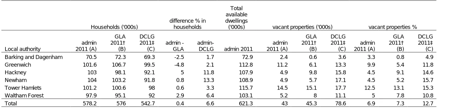
Table 2: Comparison based on total number of households by local authority using administrative, DCLG and GLA data in 000s.

Households ('000s)

difference % in households

Total available dwellings

('000s) vacant properties ('000s) vacant properties %

Local authority

admin 2011 (A)

GLA 2011† (B)

DCLG 2011‡

(C)

admin - GLA

admin-DCLG admin 2011

admin 2011 (A)

GLA 2011† (B)

DCLG 2011‡ (C)

admin 2011 (A)

GLA 2011† (B)

DCLG 2011‡ (C) Barking and Dagenham 70.5 72.3 69.3 -2.5 1.7 72.9 2.4 0.6 3.6 3.3 0.8 4.9 Greenwich 101.6 106.7 99.5 -4.8 2.1 112.8 11.2 6.1 13.3 9.9 5.4 11.8 Hackney 103 98.1 92.1 5 11.8 107.9 4.9 9.8 15.8 4.5 9.1 14.6 Newham 104 103.2 91.8 0.8 13.3 108.9 4.9 5.7 17.1 4.5 5.2 15.7 Tower Hamlets 101.2 100.6 98 0.6 3.3 115.7 14.5 15.1 17.7 12.5 13.1 15.3 Waltham Forest 97.9 95.1 92 2.9 6.4 103.1 5.2 8 11.1 5 7.8 10.8 Total 578.2 576 542.7 0.4 6.6 621.3 43 45.3 78.6 6.9 7.3 12.7 † copyright © Greater London Authority, 2011

9 Another key measure is estimates of the number of vacant properties. We define the vacant property rate as the number of households divided by the total number of residential addresses on the LLPG (Local Land and Property Gazetteer) having first removed all community establishments from the LLPG for consistency. Table 2 shows the consequential differences in vacant property rates between the three sources. These range in value from 0.8% in Barking and Dagenham using GLA definitions to as high as 15.7% in Newham using DCLG definitions.

There are two key reasons why rates may vary to this extent and in some cases appear exceptionally high. One is due to the exceptionally active regeneration in the City fringe and Docklands areas affecting mainly Tower Hamlets where there are large numbers of apartments that are as yet unoccupied. The other can be primarily traced to the lower ONS population counts on which DCLG household counts are based.

Our work in the six Boroughs produced an administrative-based population count of 1.46m, which is 0.8% higher than the GLA’s but nearly 11% higher than the equivalent count published by the ONS. However, this is not an artefact of when data were produced but a systemic problem which can be traced back in time. The London Borough of Newham is a particularly good example of this.

At the time of our work in March 2011, the published ONS population for Newham was 240k compared with our own figure of 299k. Following revisions to their methodology, the ONS released new figures in November 2011 in which Newham’s population had increased from 240k to 272k. This may be compared with figures published by the GLA which increased its own estimate for Newham from 268k to 296k in June 2011, a figure that was partly informed by our own work which by then had been made available.

The discrepancies between ONS, GLA and administrative sources are illustrative of how figures can quickly get out of kilter in areas of high in-migration and regeneration, as the case in Newham but also in neighbouring boroughs. In the approach described in the following sections we link households to population counts in a very clear and precise way which affords much flexibility over household definitions and also greater control over population counts including their validation.

Split by household type

The second issue to discuss is whether the above discrepancy feeds into and therefore distorts the breakdown of households by type. On the face of it, there is no reason why this should impact unduly as long as definitions are comparable even if the total quantum of households differs. Since local authorities are separate legally constituted decision making units we considered it more appropriate to analyse one borough in detail rather than all at once.

10

For the moment our purpose is to recreate DCLG household types using administrative sources. As was shown in Table 1, DCLG definitions are quite demanding in terms of their specificity, so reproducing these figures is likely to provide a robust test. The first critical issue to consider is the definition of a dependent child. For DCLG proposes, this is a person in a household aged 0-15 (whether or not in a family) or a person aged 16 to 18 who is a full time student (in a family with parents). However, by far the most immediate practical problem is to identify children in full time education (FTE) using administrative data.

Our key data sources were the school pupil census, in which persons are separately flagged if they are aged 16-18 and attended a school in Hackney or a neighbouring borough. They are also flagged if they are on Connexions data in which young people are as flagged as ‘FTE’ if they are in full time education (Connexions is the national information and advice service for young people that tracks young people’s intended destination from school year 8 until they are 20). However, this process is not exhaustive since there were some children receiving education in the independent sector or education in establishments located in boroughs for which we had no information.

One person households are identified as persons aged 16 or over living on their own: anyone aged less than 16 living on their own are considered to be in the category ‘other’ households. The category ‘one family and no others’ includes mixed sex couple households aged 19 and over with or without dependent children or households with only one adult aged 19 and over with dependent children.

The categories of ‘couple or lone parent with one or more other adults’ are combined into one category ‘family households with other adults and dependent children’ where these households have dependent children. In evaluating the DCLG classification system, the definition of a ‘couple’ only includes mixed sex, married or cohabiting couples, as defined by the ONS and marriage in particular may be hard to verify using administrative data except by shared surname. By the same token, same sex couples would not be considered a ‘family’ household in the DCLG classification.

A comparison of the results using DCLG figures and administrative sources is shown in Table 3. Although, as was expected, absolute numbers are lower for DCLG as compared with administrative sources for the reasons given above, the percentage breakdown turn out to be very similar for each household type. This gives us confidence that administrative sources are able to replicate the basic split in households if not the total quantum of households.

11

Table 3: Comparison of percentage of households in the London Borough of Hackney belonging to each DCLG household type using DCLG and administrative data

Household type

Administrative sources 2011

(000s) (A)

DCLG 2011

(000s) (B)

difference

(000s) (C)

% of households by type (admin)

(C)

% of households by type (DCLG)

(D)

% difference

(C-D)

Family household(couple) 20.5 18.2 2.3 19.9 19.8 0.1

Family household (lone parent) 8.6 7.7 0.9 8.3 8.4 -0.1

Family household with other adults& dependent

children 10 8.2 1.8 9.7 8.9 0.8

One person household 47.2 43.5 3.7 45.8 47.2 -1.4

Other households 16.7 14.5 2.2 16.2 15.7 0.5

12 To summarise, we find that local administrative data is able to replicate the household types in the standard DCLG classification in Table 1, suggesting that both approaches can arrive at similar results; however, the underpinning population on which government figures are based are too aggregate and out of date before they are published. In the next sections we present the case for a different approach for counting and classifying households which uses only administrative data and which deals effectively with many of these drawbacks.

2.3 Alternative household classification systems using administrative data

In what follows, our objective is to develop a new framework for counting and analysing households which is based on detailed demographic data that is extractable from locally available administrative systems. Since this data is captured in real time, household statistics, unlike DCLG figures, are synchronised snapshots at a point in time rather than projections.

We start with a brief review of the stages in the production process beginning from administrative sources of data to the creation and enumeration of household types, and finally examples of uses to inform policy and decision-making in local areas. The first stage in this approach is the prior creation of an administrative population count.

This may be conceptualised as a data base in which every person on the data base is allocated to an address or more exactly a UPRN (Unique Property Reference Number corresponding to an address and an entry on the Local Land and Property Gazetteer). The number of people and their ages then form the basis for the household classification.

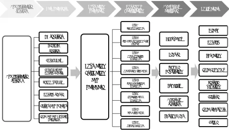
Figure 1 summarises the stages in the process that starts with a list of the administrative systems that provide the starting point for the creation of the person level data base. A technical description of this process is beyond the scope of this paper but full details may be found in Harper and Mayhew (2011a and b) and this was the method used in the Six Olympic Boroughs study of 2011. Reference 2011b, for example, provides examples of applications of the methodology to which the results set out in this paper can be considered complementary.

Since our interest in this paper is in households, we focus on the processes for aggregating person level data by age, sex or other attributes into suitable household types. In our standard classification, we define eight basic types which are defined below. The stage after this is to append to each household data pertaining to particular attributes of households such as household size, housing tenure, or benefit status. The objective is to demonstrate how easy it is to develop sub-types of households for addressing specific issues of interest.

13 Other examples that meet a specific need in local authorities include identifying workless households, children households with poor school attendance or households suffering isolation or neglect, all of which involve local authority services and responsibilities to a degree. In these cases a distinction is drawn between statistical uses of data and case management which rely on personal identification. Other attributes we have considered and developed approaches for include ethnicity identification although a discussion of the techniques involved is outside the scope of this paper.

Figure 1: Stages in the production of person and household level data and the policy domains supported Administrative systems GPregister Electoral register Council Tax

Council Tax and Housing Benefit

School pupil roll

Housing tenure

Births and deaths

Local land and Property Gazetteer Population estimation and data base Type A family households Type B single adult household with

children

Type C older cohabiting

households

Type D older person living alone

Type E three generational households Type F cohabiting adult households Type G adult living alone

Type H other households Occupancy Tenure Income deprivation Ethnicity Access to services Environment Health Housing Local economy Service provision Leisure Crime Local transport Education Administrative

sources Raw data sets Population data base classificationHousehold Analysis by attribute Policy areas

3. Enumerating household types

In this section, we lay the foundations for enumerating and analysing different household types. We start by assuming that people can be sorted into household types according to their age and the number of occupants. Based on these two variables, we show that it is possible to define both categories and sub-categories of household in a single consistent framework which can be used for multiple purposes.

14 Row one is a Type A couple household with two children and two or more adults (the additional adults could be an older sibling, friend or relative, lodgers or someone temporarily resident at an address); row two a Type B household with one adult and one child and so on. Of the examples shown, Type H households in the last two rows are the least homogenous and can be split into several sub-categories as required. In these cases the occupants are all young people (possibly students), or are from a split generation (e.g. a household in which children live with their grandparents). Note that in this classification scheme, couples may be mixed sex or same sex which can be separated out into sub-categories as required.

Type H is easily the smallest group among the standard types and may include a few households with young children and no adults. These are cases where the administrative data has identified children as living at an address but no teenage parent or adult. The most probable explanation in this small number of cases is that the adults are unregistered with a GP and do not appear on other data bases.

Figure 2: Stages in the production of person and household level data and the policy domains supported

Type A Family household with

children

2 adults and1+ children

2+ adults and 1+ children

Type B Single adult with children

1 adult and 1+ children Type C Older cohabiting couple Couple household with at least one person aged 65+ and no children Type D Older person living alone Person aged 65+ living alone Type E Three generational household

At least one person aged

0-19, one person aged 20-64, and one person aged 65+ Type F Cohabiting adult household Adult household with 2+ adults aged 20-64 Type G Adult living alone One adult aged 20-64 living alone Type H Other households Skipped generational households with older person and children but no adults Household in which nobody is aged 20+

15 Table 4: Specific examples of households defined by size and age group (Key: O

indicates a person)

Type age group 1 age group 2 age group

3 size Description

A OO-- OO ---- 4 Couple household with two children B -O-- O--- ---- 2 Single adult household with one child

C ---- O--- O--- 2 Older couple household with one person aged 65+ D ---- ---- O--- 1 Older person living alone

E --O- OO-- O--- 4 3-generational with one child ,couple and an older person F ---- OOO- ---- 3 Cohabiting adult household

G ---- O--- ---- 1 Adult living alone

H OO-- OO-- 4 Split generation household

H' OOOO ---- ---- 4 Young household (e.g. students, teenage parent)

Although administrative data cannot determine whether a couple household is a married household or whether people are related in some other way (other than by sharing a surname which is not always reliable or sufficient), for typical uses of household level data it is not essential to know this. Conversely, the ability to specify both age widths and household size offers scope to study various attributes of households in greater detail.

First we need to be able to enumerate all possible combinations by age and size of household in order to analyse their relative occurrence in the population as well as their attributes. It can be shown that the equation for the number of possible combinations N of households with r age categories and up to n people is given by:

Where n is the number of occupants (1, 2, 3, 4…n) and r is the number of age categories (1, 2, 3, 4….r). Each term inside the brackets multiplied by r gives the number of households with 1, 2, 3, 4…n people plus one further combination for the ‘void’ case where an address is not occupied and therefore undefined. The inclusion of void households is retained in resultant set of household accounts in order to derive an empty property rate for an area.

For any given value of r and n the sum of the terms gives the total possible combinations of household types. For example, there are 3+6+10+15=34 combinations of household types with 3 age categories and 4 people or 35 if the void case is included. This is shown in Table 5 row 3, which enumerates all possible combinations for up to six age categories and six occupants.

) 1 ( ! ) 1 )...( 2 )( 1 ( ... ! 4 ) 1 )( 2 )( 3 ( ! 3 ) 1 )( 2 ( ! 2 ) 1 ( ! 1 1 k r r k r k r r r r r r r r r r r

16

Table 5: Possible combinations of household demographic types based on size and age

Number of people per household (n)

number of age categories

(r) 1 2 3 4 5 6

1 1 1 1 1 1 1

2 2 3 4 5 6 7

3 3 6 10 15 21 28

4 4 10 20 35 56 84

5 5 15 35 70 126 210

6 6 21 56 126 252 462

The matrix in Table 5 is symmetrical about the diagonal so that there are the same number of combinations with j age categories and m occupants as there is with m age categories and j age categories. We can also note that each cell is the sum of the row above plus one.

For example, consider row three for up to 4 occupants the possible combinations are:

35 15 10 6 3 1 1 ₄₄ 4 1

3 = = + + + + =

+

∑

It can also be shown that the value for any particular cell is also given by:

! )! 1 ( )! 1 ( n r r n N − − + = (3)

For example, for N₄₄this is ! 4 ! 3 ! 7

=35 which is the same as the previous result.

The inclusion of gender can also be considered although this leads inevitably to more variants which can become unwieldy in general use but may be highly relevant in specific applications.

If we are only concerned with the gender mix of a household and not with gender mix within an age group, a household with 2 occupants will have 3 possible gender combinations (MM,MF,FF) and one with 3 occupants four gender combinations (MMM, MMF, MFF, FFF) and so on. This is reflected in Table 6 which shows the possible combinations of household demographic types based on size and age and gender.

17

Number of people per household (n)

number of age categories

(r) 1 2 3 4 5 6

1 2 3 4 5 6 7

2 4 9 16 25 36 49

3 6 18 40 75 126 196

4 8 30 80 175 336 588

5 10 45 140 350 756 1470

6 12 63 224 630 1512 3234

4. Classifying and counting households

Because by using administrative data age categories and occupants can be specified exactly, this provides considerable scope for analysing specific features and attributes of households. This can be illustrated using the example of a base case with three age categories and up to four occupants which has the convenient feature that it can be tabulated on one page.

In most studies to date, we have used the following age ranges 0-19, 20-64 and 65+. These are fairly broad and yet descriptively rich categories which can be fine-tuned and sub-divided into smaller age groups as required (e.g. 0-4, 5-11, 12-16, 17-19). In practice, we seek to enumerate the number of each household type in a population by specifying both the age categories and occupancy and so tables can quickly grow to a large size.

It can be postulated (and would save on analytical resources if true) that the actual distribution of household sizes and types could be replicated on the basis of a few known demographic facts, such as the sizes of each age group. If household structures were predictable or at least partly predictable from the demographic structure alone, it would be a huge simplification in many areas of activity particularly in housing, education and social services departments.

The problem is essentially one of transforming demographic data into the most household structures according to a set of rules based on a small number of demographic variables and then comparing the results with an exogenous distribution with known properties and outcomes. The aim is ambitious since much will depend on the population structure of the area being investigated (rural or urban for example), cultural and economic factors.

One way to proceed is to consider whether household patterns are the outcome of a random process (i.e. observed household patterns are simply the result of chance). Such approaches have been commonplace in geography or the natural sciences for many years and are used to determine whether processes generating a particular distribution match reality (e.g. Lewis, 1977; Rogers, 1974). If it is purely random then it means that household composition could be predicted on the basis of population demography alone.

18 address lives there independently of any other person at that address. The contrary argument is that there are societal processes such as the desire to live in families or the need to couple adults with children which cause patterns to deviate from the expected.

However, the amount by which a random process deviates from actual household patterns is itself informative and may have some predictive value. Suppose that the total population is P and the number of households is N, the average household size is P/N orλ. The expected number of households of size n is given by the Poisson distribution and the expected age composition for any level of occupancy within a sub-type is described by the multinomial distribution.

Combining both distributions we obtain the following expression for the expected number of households of size n which are split into age categoriesn₁,n₂,n₃ such that

n n n

n₁+ ₂ + ₃ =

This is given by:

3 2 1 3 2 1 3 2 1 , 3 2 1 ! ! ! ) , ,

( n n n

n p p p n n n e N n n n Np λ λ

λ = −

(4) Where N P = λ =

n household size

= i

n the number of occupants in age category i

i

p = the proportion of the total population in age category i

Continuing with our illustration, we use data from the London Borough of Hackney, one of the six London Olympic boroughs, with a population of 237,646 people at a snapshot date of 27/03/2011. Of the total population, 27.1% are aged between 0-19, 64.9% between 20-64 and 8% are age 65+. The total number of available registered addresses is 110,627 including community establishments and average occupancy of 2.148 persons per household.

For purposes of exemplification, Table 7 enumerates all possible combinations of household of up to four people in size based on the discussion in section 3 which we call the ‘base case’. We limit the example to occupancy levels of four simply to contain the size of the table so that it fits to a page.

19

Table 7: Base case enumerating household type and sub types with random assignment of people to households based on household size of up to 4 people

Case

age group

0-19

age group 20-64

age group

65+

household occupancy

household type

expected number of households

expected number of people

1 0 0 0 0 void 12,910 -

2 0 0 1 1 D 2,217 2,217

3 0 1 0 1 G 17,996 17,996

4 1 0 0 1 H 7,520 7,520

5 0 1 1 2 C 3,090 6,180

6 0 0 2 2 C 190 381

7 0 2 0 2 F 12,543 25,085

8 1 1 0 2 B 10,483 20,966

9 1 0 1 2 H 1,291 2,582

10 2 0 0 2 H 2,190 4,381

11 0 2 1 3 C 2,154 6,461

12 0 1 2 3 C 265 796

13 0 0 3 3 C 11 33

14 0 3 0 3 F 5,828 17,484

15 1 2 0 3 A 7,306 21,919

16 1 1 1 3 E 1,800 5,400

17 1 0 2 3 H 111 333

18 2 1 0 3 B 3,053 9,160

19 2 0 1 3 H 376 1,128

20 3 0 0 3 H 425 1,276

21 0 3 1 4 C 1,001 4,003

22 0 2 2 4 C 185 740

23 0 1 3 4 C 15 61

24 0 0 4 4 C 0 2

25 0 4 0 4 F 2,031 8,124

26 1 3 0 4 A 3,395 13,579

27 1 2 1 4 E 1,255 5,018

28 1 1 2 4 E 155 618

29 1 0 3 4 H 6 25

30 2 2 0 4 A 2,128 8,512

31 2 1 1 4 E 524 2,097

32 2 0 2 4 H 32 129

33 3 1 0 4 B 593 2,371

34 3 0 1 4 H 73 292

35 4 0 0 4 H 62 248

Total 42779 75798 14751 103,214 197,114

households

>4 people 7,413 40,532

20 With up to 4 occupants there are 3 distinct types of A and B households, 9 of type C, 4 of type E, and 10 of type H. Type C and Type D households are 1-person households of which by definition there is only one distinct type of each. Two final columns show the total number of households and population by household sub-type based on these data using the formula above.

Because the example only allows for occupancy of up to four people per household, it is necessary to add a residual category for households with more than four people as shown at the foot of the table. Among other things, the table highlights the fact that certain household sub-types are likely to be more common than others on the assumption of a purely random process.

For example, older households (types C and D) in which there are no children and at least one occupant aged 65+ are among the least numerous. This is because older people only comprise 8% of the total population and so are statistically more likely to live alone or in couples than in three-generational settings or households with only older people and children.

4.1 Analysis according to the eight standard types

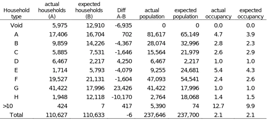
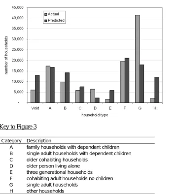
The potential utility of this table can be more readily understood if it is summarised by aggregating the information across household types. Table 8 and Figure 3 compare the expected number of households and population summarised by the eight standard household types: A, B, C etc. with the actual numbers of each type of household so that we can compare what actually occurs with a hypothesised random process.

The results show that many more adults aged 20-64 in Type G households live alone than would be the case if household formation were a purely random process. In addition, the actual number of Type B single parent households and population are substantially less than the expected number as are the number of Type E and Type H

Table 8: The actual and expected number of households and people by household type based on data from the London Borough of Hackney

Household type

actual households

(A)

expected households

(B)

Diff A-B

actual population

expected population

actual occupancy

expected occupancy

Void 5,975 12,910 -6,935 0 0 0.0 0.0

A 17,406 16,704 702 81,617 65,149 4.7 3.9

B 9,859 14,226 -4,367 28,074 32,996 2.8 2.3

C 5,885 7,531 -1,646 15,564 21,979 2.6 2.9

D 6,467 2,217 4,250 6,467 2,217 1.0 1.0

E 1,714 5,793 -4,079 9,255 24,681 5.4 4.3

F 19,527 21,131 -1,604 47,093 54,541 2.4 2.6

G 41,422 17,996 23,426 41,422 17,996 1.0 1.0

H 1,948 12,118 -10,170 2,764 18,068 1.4 1.5

>10 424 7 417 5,390 74 12.7 9.9

21

Figure 3: The actual and expected number of households by type in the London Borough Hackney (light grey = actual, dark grey = predicted)

Key to Figure 3

Category Description

A family households with dependent children

B single adult households with dependent children

C older cohabiting households

D older person living alone

E three generational households

F cohabiting adult households no children

G single adult households

H other households

households. A third observation is that many more properties would be predicted to be empty than is actually the case.

We might speculate therefore that adults much prefer to live together as couples if they have children but express a desire to live alone if they do not and assuming they can afford to do so. Alternative living arrangements such as single parent households, 3- generational households, and to some extent co-habiting adult households are all consistently fewer than would be expected by comparison which may relate to selection processes and societal norms (for example, three generational households were once much more common than they are today and single person households much less common).

22 The extent to which the actual household demographics deviate from a random process may be extended in other ways. Table 9 and Figure 4 show the actual and expected household size based on occupancy from zero to ten people. They show that the general tendency is for a greater number of households to be smaller in size than expected, the main reasons for which are firstly that fewer households than expected are empty and secondly because more people than expected tend to live alone.

Table 9: Household size and occupancy by tenure and occupancy status in the London Borough of Hackney 2011

Number of occupants

number of households

(A)

expected households

(B) diff A-B

% social housing (actual)

% benefit households

(actual)

void 5,975 12,910 -6,935 0.0 0.0

1 49,284 27,733 21,551 43.0 32.6

2 22,803 29,787 -6,984 51.3 37.7

3 12,592 21,329 -8,737 60.1 46.6

4 8,972 11,455 -2,483 63.6 50.2

5 5,107 4,921 186 69.5 56.0

6 2,608 1,762 846 70.1 60.2

7 1,371 541 830 65.9 63.6

8 753 145 608 60.7 64.5

9 482 35 447 50.4 62.0

10 256 7 249 42.6 64.5

>10 424 7 417 0.2 60.1

Total 110,627 110,633 -6 48.1 37.3

23 The size of household also affects the split between private and social housing tenure and entitlement to means tested benefits. Nearly 50% of households live in social housing in Hackney. This rate increases from 43% in single person households, rises to 70% with occupancy levels of six before falling again to 43% with occupancy levels of 10.

Means tested financial support for housing and council tax costs is paid locally through the welfare benefits system for households on low income and few assets. The table shows that the percentage of benefits households increases steadily from 32.5% in single person households before levelling at between 62% and 65% in 8+ person households.

Within this broad analysis of household types we also find that adult men and women are more likely to live in same sex than mixed households. Of households with at least one adult man or one woman present, 30% are male only and 35% female only and 35% are mixed. However a much lower proportion are same sex couple-only households. Of all households, two-person male only adult households account for 3.3% of the total, and two-person female households for 4.4%.

4.2 Age and occupancy by standard household type

Although we find that statistical distributions are not a short cut to estimating household types, they can serve a purpose as in the illustration given above. Households can also be predicted from aggregate data given more limited information such as the size of housing stock and it is possible for example to construct regression models which can do this job, although accuracy tends to be much better in some household categories than others.

24 Figure 5: Household types by average occupancy and age at output area level

In more detail:

(a) Type A family households typically contain four or five persons, including children, with an average age of 25 years and occupancy of 4.8 persons

(b) Type B single parent households range in size from two to three persons with an average age of 19 years and occupancy of 2.8 persons

(c) Type C older cohabiting households range in size between two or three persons with average age of 60 years and occupancy of 2.5 persons

(d) Type D older single person older households have an average age of 76 years upwards and become the dominant type of older household at the oldest ages

(e) Type E three generational households range in occupancy levels from four to eight people with an average age of 36 years and occupancy of 5.8 persons

(f) Type F households are cohabiting adult households with an average age of 39 years and occupancy of 2.4 persons

(g) Type G single occupancy adult households range have an average age of 40 years

0 1 2 3 4 5 6 7 8 9

0 10 20 30 40 50 60 70 80 90 Average age of occupant

A

v

er

age oc

c

upanc

y

25

4.2 Households with children

On a day to day basis local authorities are interested in households that are more likely to be users of council services. Two demographic groups that rely on the council services to a greater degree are children and older people through the housing, education, and social care and benefits systems. The following is an example based on a decomposition of households with children to show the show the relationship between the number of children per household, housing tenure and income deprivation.

Table 10 shows the frequency of households by number of children and the percentage that is social housing tenure or in receipt of means tested benefits. Of all occupied residential properties, it shows that only 30% of households have any children living in them. Of these 27.8k have fewer than 4 children and 3.2k has 4 or more. It is noteworthy that the effect of having more children is to increase the probability of being in a low income household or living in social housing.

Table 10: Number of households based on number of children in household age 0-19 in Hackney

Number of children in household age 0-19

number of households

% social housing

% on benefits

void 5975 0 0

0 73,684 45.7 33.3

1 13,732 60.2 48.5

2 9,630 63.9 53.5

3 4,420 71.1 61.7

4 1,803 71.2 66.5

5 702 63.8 71.2

6 355 53.8 73.2

7 188 38.8 77.1

8 84 32.1 79.8

9 12 33.3 83.3

10 1 100.0 100.0

>10 41 9.0 24.0

Grand total 110,627 48.3 37.5

In Hackney, for example, 48.3% of all households are in social tenure. The table shows that the chances of living in social housing increases from 45.7% with no children to 71.2% with four children after which the percentage declines. Table 10 also shows that percentage of households on benefits is 33.3% in a childless household rising to 48.5% in one-child households and steadily increasing to 83% in 9-child households.

26 In this example each household has been colour-coded according to whether tenure is private or social housing. We observe a clear clustering of households with 4+ children above row 5 and between columns D to H. We know from other work that this clustering is related to the concentration of Charedi (Ultra Orthodox Jewish) households which tend to have larger than average numbers of children. The map is hence another demonstration of the granularity of the information and the multiple uses to which it can be put.

27

4.3Minimum data sets for identifying household types including applications

As has been argued a key advantage of administrative data is that it is possible to link other attributes to household classifications. This could include information about health, education, crime or access to services and public transport. One can look at educational outcomes, access to and uptake of health services, households with unmet or complex needs, household churn and so on and so there is no doubt that a rich tapestry of detailed local information can thus be created.

We have determined that our ability to predict and therefore estimate household structures from aggregate information is limited. An important question therefore is what is the minimum administrative data sets that would be needed to produce household counts of the eight standard types? Such information could be built into policy on welfare and housing especially if it is of sufficient granularity but not overly complex to measure or define.

Where available we would be able to identify single parent households and older households as being not only among the more vulnerable groups but also gaps or similarities with other household types. In essence we thus seek a set of markers of identifiers with which to flag each household in such a way they these can be used in combination to produce the eight standard types.

Furthermore these markers, or risk factors, would be predictive in terms of their ability to identify some attribute or other of those households. For purposes of illustration we choose income deprivation as this attribute and we use benefit status as our proxy for defining it. They are: presence of a child aged 0-19, an adult aged 20+, at least one person aged 65+, and another aged 20-64. Since housing tenure and income deprivation are also co-related we define a fifth risk factor as ‘living in social housing’.

Of these factors the first four demographic factors are sufficient to transform demographic data into household counts of the eight standard types. The method is general and does not have to rely on administrative counts of the population and could be produced during the early stages of processing of census data in order to produce compact statistical counts at sub-local authority level. The fifth factor is added since our focus in this case is on income deprivation and inequality among households.

28

Table 11: Breakdown of household types by risk factor combination and risk of income deprivation

Case

house-hold

type frequency

any child age single adult age 20+ at least one person age 65+ at least one person aged 20-64 living in social housing Observed % of households on benefits 0-19

1 H 76 Y Y Y Y 88.2

2 D 4,979 Y Y Y 80.2

3 E 1,139 Y Y Y Y 72.4

4 C 3,073 Y Y Y 71

5 B 6,482 Y Y Y Y 70.8

6 H 14 Y Y Y 64.3

7 C 813 Y Y 63.2

8 A 11,170 Y Y Y 60

9 H 705 Y Y 52.5

10 E 575 Y Y Y 49

11 D 1,488 Y Y 48.8

12 G 15,700 Y Y Y 46.7

13 H 28 Y Y Y 46.4

14 B 3,377 Y Y Y 45.1

15 F 9,094 Y Y 43

16 H 10 Y Y 40

17 C 1,575 Y Y 35.9

18 A 6,236 Y Y 33.1

19 C 424 Y 25.5

20 H 1,115 Y 24.8

21 F 10,433 Y 16.1

22 G 25,722 Y Y 13.9

Total 104,228 30,927 57,852 14,194 94,576 53,245 39.6

The rows in the table are arranged such that the most probable sub-group in terms of income deprivation is row 1. Of the 76 households in this category 88.2% are households on benefits whereas in row 22 of the 25,722 Type G households only 13.9% are on benefits. This compares with 39.6% of households for Hackney as a whole. Hence this is a wide spectrum of households that fall into greater or lesser income deprivation if benefits status is used for measurement purposes.

The column totals represent the number of households to which the given risk factor applies so for example 30,927 households have at least one child living in them and 53,245 households are social tenure. The estimated value of each risk factor for predicting income deprivation can be obtained using logistic regression techniques. We set up the following model in which we regress the logit of living in a household on benefits against each of the grouped risk factors as follows.

i mi m M m m i i

i x u

r r

L _= + +

29

where i is the ith _{factor combination, i=1,22 and M is the number factors in the}

model, M=5, and Li

^

is the sample log-odds in category i of a reported DV occurrence.

This results of the regression given in Table 13. They show that the odds of living in a household on benefits increase 4.3 times if living in social housing, 3.4 times if a person resident is age 65 or over, 2.6 times if there are children living in the household and 1.3 times if there is a single adult aged 20 or over. If there is an adult age 20 to 64 the odds are reduced by 0.9 which is related to the fact that this is peak working age. All the estimates are significantly different from zero at the 95% level of probability.

Table 13: odds of income deprivation by risk factor including 95% confidence intervals

Risk factor

parameter

estimate odds ratio

lower CI

upper CI

Any child 0-19 0.95 2.6 2.5 2.7

Single adult 20+ 0.26 1.3 1.26 1.33

At least one person age 65+ 1.24 3.4 3.3 3.6

At least one person aged 20-64 -0.08 0.9 0.87 0.98

Living in social housing 1.4 4.2 4.1 4.4

Constant -1.77

The odds are multiplicative so that a household with an older person living alone in social housing is 1.3 x 3.4 x 4.2 = 18.6 times more likely to be in receipt of benefits than a household with none of these risk factors based on this example. Figure 7 shows the predicted percentage of households versus the observed percentage. The fitted equation has a value of R2 of 0.86 and the slope of the equation is 1.00 indicating a very model fit.

Figure 7: Expected percentage of households on benefits based on risk factors versus actual percentage by risk group (R2 =0.8557)

0 10 20 30 40 50 60 70 80 90 100

0 10 20 30 40 50 60 70 80 90 100 observed %

pr

edi

c

30 The significant correlation with social housing is observable in the bubble chart in Figure 8. On the vertical axis is the percentage of households in receipt of means tested benefits and on the horizontal axis is the standard household type. Each numbered colour coded bubble corresponds with a row in Table 12 in which the size of the bubbles is proportional to the number of households in that sub-category.

For any given household type the higher bubble corresponds to households in social tenure and the lower bubble in private tenure so the correlation between social housing and income deprivation is quite stark in this borough. Although not shown here these results can be mapped in various ways to show more and less affluent neighbourhoods, income poverty among the different standard types, or income poverty in household with or without children etc.

Figure 8: The relationship between the percentage of households on benefits and household type by risk category

5. Implications and critique

This paper has identified a significant gap in the availability and quality of household statistics at local level. Despite the diversity in sources of information available, this information is only available in the form of national surveys or data down to district level. For methodological reasons and lags in reporting, we have shown that figures have a tendency to be distorted especially in areas of high population growth and churn.

31 On the other hand DCLG district level household projections fulfil a purpose in that they provide consistent national and regional projections (Department for Communities and Local Government, 2008; March 2010b). Revisions to the DCLG methodology and outputs have also resulted in improvements including projections for the number of households with dependent children, based on revised ONS population and migration estimates (Department for Communities and Local Government, 2008; March 2010a; March 2010b; August 2010; November 2010).

They are extensively used by government departments, the National Housing and Planning Advice Unit, regional planning bodies and local authorities (Department for Communities and Local Government, March 2010b), and in work done on future housing need by among others the Cambridge Centre for Housing and Planning Research for Shelter, the Town and Country Planning Association, and the Joseph Rowntree Foundation (Holmans, 2012).

However DCLG projections are clearly not ideal, as demonstrated by the GLA’s use of alternative population evidence for London for their household projections, from the higher administrative data counts in Table 2, and from general literature on dissatisfaction with ONS mid-year population estimates (House of Commons Treasury Committee, 2008). In addition, the statistics are in reality forecast counts and not actual counts of households, whilst definitional types are fixed and inflexible.

Surveys by contrast fulfil a need at national level and are widely exploited in social research and frequently form the evidence bases in policy domains such as welfare policy or child care. However, again they are not something that can easily be used for other purposes especially by local users since they are not geographically disaggregate or timely enough to be representative, and nor can they be easily linked to other data.

The gaps that this paper exposes are, to a limited extent, being filled by one method or another as evidenced by the commercial systems that are available such as Mosaic. Unlike DCLG data, these are available at a sub-district level and are therefore an improvement. However, because they also rely to a large degree on government census data their accuracy is also questionable and are lacking in detail as regards demography and occupancy.

One important catalyst for change is the Localism Act (2011) which gives local authorities more freedoms including responsibility for their own Local Development Framework. This often means finding evidence beyond or even contrary to the DCLG figures to be more locally representative (e.g. Leeds City Council, 2011).

In addition there are new demands required for statistics for evidence required under the Localism Act and the Health and Social Care Act (2012). The latter will bring into being Health and Wellbeing Boards. These will be a forum for local commissioners across the NHS, public health and social care, elected representatives, and others with responsibility to draw up Health and Well-Being strategies and plans.

32 locally relevant and therefore better able to support these new duties on local authorities in areas ranging from health care provision to social and leisure services.

Our data have been used in a number of studies in which accuracy timeliness and specificity are important. This include work on complex families, overcrowding, health assessments, access to and uptake of services including unmet need, educational outcomes, and a range of health studies including costs of secondary care by household type, access to child care and so on.

In this paper we have not attempted to create future household projections from administrative data, but this may be considered. A basic requirement is to recreate the data at intervals and to identify trends within the population and household types. For example, work has already been conducted on analysing population change and household formation in the six Olympic boroughs, with encouraging results.

6. Conclusions

Household level statistics about the size, type and demography of households are seen as increasingly important in a range of applications. As well as forming the backbone of evidence for assessing future housing need, household level data is useful for designing services, predicting consumption patterns and generally informing policy in areas such as welfare benefits, childcare and taxation.

The premise of this research is that current sources of information used in each of these areas are inflexible, fragmented and piecemeal. A key consequence of this is that the availability of information especially at local level is limited. This is impacting on local authorities’ ability to conduct its business efficiently and effectively in terms of policy development and service delivery.

With new duties placed on local authorities, for example as a result of the Localism and Health and Social Care Acts, this is likely to highlight further the present unsatisfactory position and lead to demands for better data. At present it seems unlikely that this gap can be filled by either the ONS or other government departments because of a lack of resources and other priorities.

This is unfortunate as is it is local authorities that are most likely to benefit from better household data. On the other hand this paper has shown that the considerable administrative data sets available to local authorities could be put to much better use. It has described how these assets can be used first to provide detailed population estimates and secondly how these estimates can be used to convert population into households.

33 Our results showed that our methodology could replicate the existing DCLG typology accurately on a proportionate basis. The main issue for DCLG to address is that the population data on which their household methodology is based undercounts the number of households in the six London boroughs as compared with our figures and the Greater London Authority’s.

We find that this weakness is due primarily to the ONS demographic estimates which are part of DCLG’s household methodology. This is apparent not only from direct comparisons with our own estimates and GLA’s but also from the considerably higher empty property rates when household counts are compared with the number of dwellings.

However, even if DCLG’s estimates had been more accurate and closer to ours there would still be problems with the lack of flexibility over definition and geography and in the capacity to link with other important household variables. In contrast, our method of creating household counts and types is able to offer flexibility in these aspects, and draws upon actual current population counts rather than estimated trends, thereby reflecting a more accurate population.

The approach adopted demonstrates that individual households can form the building block of any geographical area of interest and be linked to any other household level variable, and so this also bypasses the need for expensive surveys to a degree. Surveys seeking opinions or personal habits such as smoking or drinking behaviours are a different matter of course. Even in these cases the results can be linked to administrative data as appropriate although by definition it would only include a sample of all households.

At this point the methodology cannot currently verify the marital relationships between residents of a household, and nor has this aspect been evaluated in terms of accuracy or consistency against national household figures. This would require us to link records on marriage and divorce which, even if available electronically, would not contain the current address or personal identifiers to enable this and would pose formidable legal and practical challenges.

It is debateable whether this gap is an important omission or not when compared against the other advantages that are available, especially an ability, demonstrated in the Olympic Boroughs study, to link other local data sources including health and social services data, leisure services and many other sources to provide a single statistical platform for use locally.