City, University of London Institutional Repository
Citation
:
Broom, M. and Cannings, C. (2015). Graphic deviation. Discrete Mathematics,
338(5), pp. 701-711. doi: 10.1016/j.disc.2014.12.011
This is the accepted version of the paper.
This version of the publication may differ from the final published
version.
Permanent repository link: http://openaccess.city.ac.uk/7802/
Link to published version
:
http://dx.doi.org/10.1016/j.disc.2014.12.011
Copyright and reuse:
City Research Online aims to make research
outputs of City, University of London available to a wider audience.
Copyright and Moral Rights remain with the author(s) and/or copyright
holders. URLs from City Research Online may be freely distributed and
linked to.
M. Broom1,∗ and C. Cannings2
1
Department of Mathematics, City University London, Northampton Square, London EC1V 0HB, UK.
2
School of Mathematics and Statistics, The University of Sheffield, Hounsfield Road, Sheffield, S3 7RH, UK.
*corresponding author
Abstract. Given a sequence ofnnonnegative integers how can we find the graphs which achieve the minimal deviation from that sequence? This extends the classical problem regarding what sequences are “graphic”, that is, can be the degrees of a simple graph, to issues regarding arbitrary sequences. In this context, we investigate properties of the “minimal graphs”. We shall demonstrate how a variation on the Havel-Hakimi algorithm can supply the value of the minimal possible deviation, and how consideration of the Ruch-Gutman condition and the Ferrer diagram can yield the complete set of graphs achieving this minimum. An application of this analysis is to a population of individuals represented by vertices, interactions between pairs by edges and in which each individual has a preferred range for their number of links to other individuals. Individuals adjust their links according to their preferred range and the graph evolves towards some set of graphs which achieve the minimal possible deviation. This Markov chain is defined but detailed analysis is omitted.
Keywordsdegree-preferences, graphic sequences, Havel-Hakimi, Ruch-Gutman, Ferrer diagram.
1. Introduction
Forn∈N(Nbeing the set of nonnegative integers), we consider the setSnofn-element sequences
u= (u1, u2, . . . , un) where (n−1) ≥u1, u2. . . ui, ui+1. . . un ≥ 0. There is a considerable body
of work [2],[3],[4],[5],[6] addressing the question of which elements of Sn are graphic, that is for
whichu∈Sn does there exist a simple graph whose vertices have precisely the degrees (number
of neighbours) ui; there may exist more than one. We shall denote the set of graphic sequences
by Hn. However, there is, to our knowledge, nothing addressing the question of “how far from
graphic” a member ofSnis.
Suppose we have a set ofn individuals labeled{1,2, . . . , n}, and that associated with vertexi is a pair of integers 0 ≤mi ≤Mi ≤(n−1). We investigate whether there are simple graphs on
these n vertices with degrees ui such that mi ≤ ui ≤ Mi, and more generally what graphs are
closest to achieving these inequalities in a sense defined below. This investigation is facilitated by introducing a process on the possible graphs which we index witht, and refer tot as time. Thus suppose at timetthere exists a graph withnvertices,Xt. We denote a state of the system by the n×nadjacency matrixX = (xij) (thusxii= 0, xij= 1 if there is an edge (i, j) and is 0 otherwise).
We writeXt=xwhenXt is a graph with adjacency matrixx. The sequence associated with the
graphxisu, where theith element ofu, ui, is the degree of theith vertex ofx. Ifmi≤ui ≤Mi
we say that vertex i isNeutral in which case no action is taken, ifui < mi we say vertex i is a
Joiner and then, if possible, we selects a vertexj to which it is not currently linked and add the edge (i, j) to it, while ifui > Mi then iis said to be aBreaker and then, if possible, we select a
vertex j to whichi is currently linked and remove the edge (i, j). We refer to this new graph as
Xt+1. We refer to this step as atransition and the new graph is potentially nearer to achieving
the set of inequalities on the degrees. Here we restrict ourselves (in the main) to the case where
mi = Mi for all i, refer to the sequencea = (a1, a2, . . . , an) ∈ Sn where ai = mi = Mi as the
target, and toai as i’s target.
1.1. Definitions.
Definition 1. For two sequences uand v in Sn the Distancez(u,v) = Σni=1|ui−vi|, i.e. z is
the distance generated by theL1 norm.
Recall thatHn⊂Snis the set of graphic sequences. Now suppose that we consider targeta∈Sn.
We are interested in the distances between a and the graphic sequences, Hn. We introduce the
notion of a score of a sequence.
Definition 2. The Scoreofa iss(a) =minu∈Hnz(a,u).
Thus s: Sn → {0,1, . . . , kn}, where kn =dn/2ebn/2c which occurs for the cases where we have dn/2eor bn/2ctargetsn−1 and the remainder 0. We prove that the transitions for a particular targetalead to a subset of the possible sequences with minimal distance from the target. We refer to this as the minimal set ofadefined as follows.
Definition 3. The Minimal Setofa isJ(a) ={u∈Hn|z(u,a) =s(a)}.
Although we are focusing on the situation where we havemi=Mi for every vertex, we relax this
condition for the moment as theorems 1 and 2 below are valid in the more general case. For this purpose we introduce the term deviation to take the place of our distance/score in the restricted case.
Definition 4. If the degree of vertex i is ei, then we define the Deviation i of that vertex by
i=max[(mi−ei),(ei−Mi),0].
and
Definition 5. The deviation of the graph Xt is defined asΥt= Σni=1i.
We refer to a vertex as a Neutral, a Joiner or a Breaker, according asi is 0,mi−ei orei−Mi.
For a targeta, it is clear that the deviation of a graphxis the same as the distance of its associated sequenceufrom the target, and so the minimum deviation from the target over all graphs is simply the score.
This section is central to understanding the underlying population aspects that constitute the applications of our model, but is not necessary for any readers only interested in the graph-theoretical aspects, who can skip it and move straight to the sections that follow, starting with Section 3.
Section 3 considers the structure of minimal graphs with respect to a specific target. Any minimal graph, with respect to a specific target, has each vertex classified as a Joiner, a Breaker or Neutral. Our fundamental result is Theorem 4, which demonstrates that for a given sequence the minimal graphs are characterized by the absence of certain patterns of presence and absence of edges. From this we can deduce certain local patterns and demonstrate a certain partition of the vertices in minimal graphs, as shown in Theorem 7. These ideas may help identify and enumerate the possible sets of minimal graphs.
Section 4 demonstrates a method for finding the minimal score for a given sequence. We address the question of finding the minimal score for a given target, and do this through a variant of the classical Havel-Hakimi algorithm [2],[4], see Theorem 8. We finally address the issue of identifying all the minimal graphs for a given target using the Ferrer diagram [7], and exploiting the Ruck-Gutman [6] conditions. We prove that the set of Ferrer diagrams corresponding to minimal graphs for a given target is connected under valid transitions (Theorem 13), and moreover that the set of minimal graphs is connected (Theorem 14) except possibly when the score is zero.
2. Sequences, transitions and a Markov process
2.1. Markov Chain model. We introduce here a population model; there are n individuals, represented by the vertices of a graph, where individual i wishes to link to between mi and Mi
others. Supposing at timetthat the graph isXt, and that individualiis selected with probability pi. A transition is then made, as described earlier, where the edge to add or subtract is selected
at random with equal probabilities. The process Xt is a homogeneous Markov chain with the
following transition probabilities:
1) For any graphx∗, with sequenceu, which differs fromxin a single entry, wherexij= 0, x∗ij = 1
for somei, j,
P(Xt+1=x∗|Xt=x) =
pin−11−ui +pj 1
n−1−uj ui< mi, uj< mj
pin−11−ui ui< mi, uj≥mj
pjn−11−u
j ui≥mi, uj< mj
0 ui≥mi, uj≥mj.
2) For anyx∗ which differs byxin a single entry, wherexij= 1, x∗ij= 0 for somei, j,
P(Xt+1=x∗|Xt=x) =
piu1i +pju1j ui > Mi, uj> Mj
piu1i ui > Mi, uj≤Mj
pju1j ui ≤Mi, uj> Mj
0 ui ≤Mi, uj≤Mj.
3) For anyx∗, differing fromxin two or more entries, P(Xt+1=x∗|Xt =x) = 0.
Theorem 1. For any set of ranges [mi, Mi] Υtis non-increasing, under the possible transitions,
witht.
Proof.
Consider the transition from timet to timet+ 1. When a vertexiis selected then if it is Neutral no change happens so Υ(Gt+1) = Υ(Gt). If it is a Joiner then its deviation is decreased by 1 (since
an edge is added), and if that edge is joined to vertexj then the deviation of that vertex changes by−1, 0 or +1 according as (a)uj < mjsojis a Joiner, (b)mj ≤uj≤Mj−1 sojis a Neutral or
(c)uj =Mj sojis a Neutral, orMj< uj soj is a Breaker. Thus Υ(Gt+1)−Υ(Gt) is respectively −2,−1 or 0. A similar argument applies if we pick a Breaker.
Corollary 1.1. Whenmi=Mi alli thenΥ(Gt+1)−Υ(Gt)is−2 or0.
Proof. Case (b) from the proof of Theorem 1 is then impossible.
Corollary 1.2. If there is a path of transitions from a graph state x to another with a lower deviation, thenx is a transient state, and soP(Xt=x)→0.
The state space can be partitioned into a set of transient states, and some number of connected closed setsS1, S2, . . . , Sk, the absorbing sets.
In Section 2.3 we define the transition graph. This is a directed graph and the setsS1, S2, . . . Sk
are the strongly connected subsets of that graph.
Corollary 1.3. Each graph within a closed set has the same deviation.
The states within each set communicate (i.e. any such state can be reached from any other) since the set is connected, so by Theorem 1 the states within any set have the same deviation, denoted by Υ(Si). Since there are only a finite set of sets there is a minimum value. Our next theorem
establishes that each set achieves this minimal deviation, which we denote bydm. Theorem 2. The deviation of any graph in any of the absorbing sets isdm.
Proof.
SupposeG1 andG2 have Υ(G1)>Υ(G2).
We defineδij = 0 ifG1 and G2 both have the edge (i, j), or neither of them do, and else define
δij= 1. We then define ∆ = Σi,jδij. We attempt to decrease ∆ by making a valid transition from
G1.
Consider a Joiner, isay, inG1. Suppose we can add an edge (i, j) toG1 which is present inG2,
then ∆ will decrease. We will be unable to do this only if all (i, j) not inG1 are also absent from
G2, which implies thati is a Joiner inG2 with a deviation at least as large as inG1.
In a similar manner we consider a Breaker,isay, inG1. If we can remove an edge (i, j) fromG1
which is absent fromG2 then ∆ will decrease. We will be unable to do this only if all (i, j) inG1
are also present fromG2, which implies thatiis a Breaker inG2 also with a deviation at least as
large as inG1.
Thus we can reduce ∆ unless every i has a deviation at least as large in G2 as in G1, which
contradicts the assumption that Υ(G2)<Υ(G1). Repeating the process eventually the score will
2.3. The Transition Graph. A graph of interest is that describing the possible transitions be-tween graphs Xt induced by a specific target a. In order to do this we need to expand the set
Hn, which has non-increasing elements, to encompass all permutations of these orderings; call this
set H∗
n. Now given a target a, we define an equivalence relation ∼on H∗n. We write P(u) for
the action of the permutation operatorP onu. SupposeYis the set of permutations which leave
a unchanged, then for u∈H∗n and v ∈ H∗n, u∼ v if and only if for all P ∈Y, u=P(v). We then choose a set of representatives H†n, that is one element from each equivalence class, which will correspond to the vertices of our transition graph.
Suppose thatuandv, inHnare such that for specificiandjwe haveui=vi+ 1,uj =vj+ 1 and
uk =vk otherwise. Now under the model for transitions described earlier a transition is possible
fromutov ifui < ai oruj< aj, and fromv touifvi> ai orvj> aj. We define the transition
graph Tn ={H†n(a),Fn(a)} where Fn(a) is the set of possible transitions defined above; these
edges are directed.
Givena, associated with each vertexuinTn(a) is the distanced(u,a). The transitions are of two
types, those where the degrees of both the vertices which are affected move towards their target, so the score drops by 2, and ones where one moves towards and one away from its target when the score does not change. If, and only if, the transition is of the second type then there is also a transition in the reverse direction. Moreover, as we proved above in Theorem 2, it is always possible to move from a state to one with a lower score if such exists, though this may involve multiple steps. The system therefore will ultimately reach one of the graphic sequencesufor which
d(u,a) is minimal. If that score is zero, which only occurs when the target is itself graphic, then no further moves are possible. If the score is other than zero then the state can move around withinJ(a), and we prove that the graph induced by the verticesJ(a) withinTn(a) is connected.
This is not to assert that the set of corresponding graphs can all communicate; for example if
a= (2,2,2,2) so thatJ(a) has a single element (2,2,2,2) then no movement is possible, but there are three graphs corresponding to this degree sequence between which there is no communication. The transition diagram can be obtained for givennand some specific target in the following way. We construct the set of possible permutationally distinct graphic sequences for that n and that partition. Then we join, in the graphTn(a) those sequences which differ by +1 in two positions,
or by−1 in two positions. Note that this is always possible for any target, since clearly the target must differ from one of the sequences in the positions which are changed, and so there will be the possibility of incrementing or decrementing the position appropriately. Finally we can add the directions appropriate for the specific target by calculating the deviations, arrows going on every edge in the direction of non-increasing score.
3. The Breaker-Joiner structure of minimal graphs
This section addresses the question of the structure of minimal graphs. It is clear that every graph is the minimal graph for some non-empty set of targets since trivially it is a minimal graph whose target matches its degree sequence. It is also clear that it is a minimal graph for any target at distance 1, and also for any target at distance 2 provided that target is not itself graphic. A more general question is to characterize in some way the set of possible targets for which a given graph is a minimal graph.
occurs we can trace back the set of transitions which led to that reduction. We encapsulate the possibilities in the following definitions.
Definition 6. An Alternating Edge Sequence (AES) for a graphGwith edge set Eis a sequence
{v1, v2, . . . , vr} wherevi6=vj for all1≤i < j≤nwith the possible exceptionv1=vr, and
(a)(vi, vi+1)∈E foriodd and (vi, vi+1)∈E fori even or
(b)(vi, vi+1)∈Efori odd and(vi, vi+1)∈E forieven.
Definition 7. An Improvable Alternating Edge Sequence (IAES) for a graph G with respect to a given target is an AES {v1, v2, . . . , vr}, defined by the following conditions (here Jis the set of
Joiners inG,N the set of Neutrals, andB the set of Breakers), (1) if 1< i < r thenvi∈N,
(2) if (v1, v2)∈E thenv1∈B, elsev1∈J,
(3) if (vr−1, vr)∈E thenvn ∈B, elsevn∈J.
In the case where v1=vr we require thatr is even and that the deviation ofv1≥2.
Theorem 3. If r >2 and{w1, w2, . . . , wi−1, wi, wi+1. . . , wr−1, wr} is an IAES then exactly one
of {w1, w2, . . . , wi−1, z} and{z, wi+1, . . . , wr−1, wr} is an IAES where z is a Joiner. Similarly if
z is a Breaker.
Proof.
The proof relies on the fact that if an IAES has ends of common type, i.e. both Joiners or both Breakers, then the number of terms is even, and if the ends are of distinct types then it is odd. Ifw1 andwrare both Joiners, or both Breakers, thenris even, and hence one of (r−i+ 1) and
i is odd and one even. Hence whether z is a Joiner or a Breaker, there will be an IAES in one direction fromz, but not in the other. Note that ifw1=wr so that the AES is of type (3) or (4)
in Definition 7 the result still hold.
Ifw1 and wr are different, i.e. one a Joiner and one a Breaker, then ris odd, and hence both of
(r−i+ 1) andiare even, or both odd. Hence whetherzis a Joiner or a Breaker, there will be an IAES in one direction fromz, but not in the other.
If a is graphic then there can exist no IAES’s since every vertex is Neutral. For non-graphic sequences we have the following fundamental theorem.
Theorem 4. A graphGis minimal with respect to some non-graphic targetaif, and only if, there are no IAES’s.
Proof.
(1)Gis minimal implies that there are no IEAS’s.
Suppose G is minimal with respect to a and there exists an IAES. If r = 2 then we have an immediate improvement sincev1 and v2 are both Breakers, or both Joiners. Forr >2 in each of
the four cases above we can make a valid transition usingv1 andv2 with no change in the score,
and following the transition the sequence{v2, v3, . . . , vr} will be an IAES in the new graph. We
make transitions until we are left with onlyvr−1andvr, and these vertices will be of the same type.
Note that in the case wherev1=vrthe first vertex retains its type during the first transition since
its score initially was≥2. Thus the final transition will decrease the score by 2, which contradicts the fact thatGis minimal. Thus there can have been no IAES’s.
(2) There are no IEAS’s implies thatGis minimal.
Consider any transition, which clearly can make no change to the score since there are no Breaker-Breaker edges, or Joiner-Joiner non-edges. We prove that there will be no IAES subsequent to any change. Suppose without loss of generality that we delete an edge between vertexv1, a Breaker,
and vertexv2 (adding an edge between a vertexv1, a Joiner, and a vertexv2 will have reciprocal
consequences in the arguments below). Thenv2 must be a Joiner after the change.
Following the change there are various candidates to be IAES’s; clearly only those which involve
v1,v2or both. We establish that the existence of an IAES after any switch implies that there was
an IAES before the switch, a contradiction.
We knowv2 is a Joiner after the switch so must be at the end of any IAES of which it is a part.
We first consider the three possibilities in whichv2is part of a new IAES.
(i) Consider any sequence {v2, w1, . . . , wr}, where wr 6=v2 and v1 does not occur. If this is an
IAES then it would have originally have been one if v2 had originally been a Joiner, while if v2
had been Neutral then{v1, v2, w1, . . . , wr} was already an IAES.
(ii) Consider any sequence {v2, w1, . . . , wr, v2}, where r is even, which does not contain v1, so
after the switch v2 is a Joiner with score ≥ 2. If before the switch v2 had a score ≥ 2 then {v2, w1, . . . , wr, v2}was already an IAES. In the case where the score of v2 was previously 1 then {v2, w1, . . . , wr, v2, v1} was already an IAES.
(iii) Consider a sequence including bothv1 andv2. We need to consider the two possibilities for
the state ofv1after the switch.
(a) Suppose v1 is Neutral after the switch, then the candidate to be an IAES is of the form {v2, . . . , v1, . . . , wr}, and thus by Theorem 3 either {v2, . . . , v1} or {v1, . . . , wr} was already an
IAES.
(b)Suppose v1 is still a Breaker, then the IAES must be {v2, . . . , v1}, and the number of terms
must be odd. If v2 was originally a Joiner then {v2, . . . , v1} was already an IAES, whereas if it
were neutral then {v1, v2, . . . , v1} was already an IAES since we know that v1 had a score of at
least 2 before the switch since it remained a Breaker.
(iv) Consider any IAES which does not includev2, and hence must includev1. If this is{v1, . . . , wr}
then v1 is still a Breaker and so the same sequence was an IAES before the change. The same
argument applies for {v1, . . . , wr, v1}. If this is {w1, . . . , v1, . . . , wr} then this requires that v1
changed to Neutral, so either{w1, . . . , v1} or{v1, . . . , wr}was an IAES originally, by Theorem 3.
Thus no change can create a graph with an IAES, so no graph can be reached for which the score can be reduced and thus by the argument of Section 2.2, the graph is minimal.
The above necessary and sufficient condition provides us with a variety of local conditions, which are illuminating regarding the structure of a minimal graph. We list some of these. In each case an IAES is key but is not made explicit.
Corollary 4.1. For any minimal graph the following properties hold. (1) No two Breakers are joined.
(2) Every pair of Joiners are joined.
(3) If a Neutral is joined to a Breaker then that Neutral is joined to every Joiner ⇔ if a Neutral is not joined to some Joiner then that Neutral is not joined to any Breaker.
(5) Suppose that some Neutral N is not joined to some Joiner, and another Neutral N∗ is not joined to some other JoinerJ∗ thenN is not joined to N∗.
Theorem 5. For any targetathe minimal setJ(a)contains at least one member with no Joiners, and at least one with no Breakers.
Proof.
Consider some targeta. Ifais graphic then the set of minimal sequences consists ofa alone, and this will have no Breakers and no Joiners so the theorem holds in this case.
Now suppose a is not graphic. We now prove that there exists a minimal graph which has only Breakers and/or Neutrals with respect toa. Choose any minimal graph with at least one Joiner. If this is not possible then, since the set of minimal graphs cannot be empty, there is a minimal graph with no Joiners. For the case where there exists such a minimal graph we successively add edges to the Joiners. This will be possible provided there is a Joiner which is not joined to every other vertex. This is always the case since a Joiner joined to every other vertex would imply a degree, for that Joiner, of n−1 which is the maximal possible degree and hence contradicts the fact that that vertex is a Joiner. We can thus proceed until all Joiners have been removed. The argument to establish that there is a minimal graph with no Breakers proceeds in a similar manner removing edges from Breakers and observing that a vertex with degree 0 cannot be a Breaker.
Theorem 6. For a minimal graph the degree of a Joiner is greater than or equal to that of a Breaker.
Proof.
Consider the set consisting of all the Joiners and all of the Neutrals which are linked to a Breaker; these latter are linked to every Joiner. Denote this set byH and|H|=k. Now we know from (2) and (3) of the above corollary that each Joiner is linked to every other element of H. Thus the degree of every Joiner is at leastk−1; it may be larger since it may be linked to Breakers and to other Neutrals which are not themselves linked to any Breaker. Now each Breaker is linked only to some subset of H, by Corollary 4.1, so its degree is less than or equal tok. If it is equal to k
then it is linked to every Joiner which therefore themselves have degree at leastk, thek−1 links withinHand the link to the Breaker, otherwise the Breaker’s degree is at mostk−1.
Corollary 6.1. With respect to the ordered target the Joiners precede the Breakers for any minimal graph.
Proof. Since the degree of any Joiner is at least as large as that of any Breaker, and the target of a Joiner is greater than the degree, and that of a Breaker is less, the target of a Joiner must strictly exceed that of any Breaker.
It is intuitively reasonable that those vertices (individuals) with higher targets will fall short while those with lower targets will exceed them.
From the above we have the following structure for a Minimal Graph.
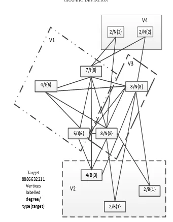
Theorem 7. For a minimal graph with respect to a specific target the vertices can be partitioned into five subsets (some of which may be
V2 - an independent subset which contains the set of Breakers,
V3 - a subset of Neutrals each of which has at least one link to a Breaker and each is linked to all the Joiners,
V4 - a subset of Neutrals which are not linked to every Joiner and each is not linked to any Breaker,
V5 - a subset of Neutrals each of which has no links to any Breakers and is linked to every Joiner.
Proof.
This follows directly from Corollary 4.1.
Figure 1 illustrates the partitioning for the target{8886632211}. 4. Finding the Minimal Deviation
In order to find the minimal deviationdm we could examine all possible graphs for given n and
evaluate their deviations. However, there are more efficient methods which give the deviation for any specified target (i.e. where for alli,mi=Mi).
We shall give two simple methods of deriving the minimal deviation. The first is based on the algorithm of Havel [4] and Hakimi [2] which allows one to check whether a given sequence is graphic, and also generates an example of such a graph. The second method exploits the ideas of H¨asselbach and Ruch-Gutman.
4.1. The Havel-Hakimi Algorithm. Given a sequence one applies an algorithm introduced by Havel [4] and Hakimi [2], which either produces a simple graph with the desired degree sequence, or fails in which case the sequence is not graphic.
The Havel-Hakimi algorithm is as follows. Suppose one has a sequence of degreesd={d1, d2, . . . , dn}
wheredj ≥dj+1≥0 for 1≤j≤(n−1). Ifd1>0 anddd1+1≤0 then the sequence is not graphic.
Assuming d1 >0, if dd1+1 ≥1 then replace the degree sequence by{d2−1, d3−1, . . . , dd1+1−
1, dd1+2, . . . , dn}; essentially connect the vertex with highest degree to those others with next
highest degrees, then eliminate d1 from the sequence, reorder the new sequence (if necessary) in
decreasing order, and take this as the new sequence which we need to check to see if it is graphic. Apply this process recursively. If this can be done until one arrives at a sequence consisting entirely of 0’s then the sequence is graphic.
4.2. Reordered Havel-Hakimi Algorithm. We introduce a new algorithm which is a slight modification of the Havel-Hakimi algorithm which has an easier application in subsequent proofs. In the Havel-Hakimi algorithm one reduces the elements in positions 2 throughd1+ 1 by one, and
then reorders to obtain a decreasing sequence. Reordering is required if there is a substring of the original sequence,s, of more than one equal elements which begins at, or before, thed1+ 1’st
element and extends beyond it. Here we avoid the reordering step in the above case by instead subtracting ones from the elements at the end of this strings.
Formally, suppose one has a sequence of degreesd={d1, d2, . . . , dn} wheredj ≥dj+1 for 1≤j≤
4
V2
7/J{8}
5/J{6}
2/B{1}
8/N{8}
4/B{3}
2/B{1}
Target
8886632211
Vertices
labelled
degree/
type{target}
4/J{6}
8/N{8}
2/N{2}
2/N{2}
V3
V4
[image:11.612.170.511.99.536.2]V1
Figure 1. A minimal graph for the target 8886632211 separating the Joiners V1,
the Breakers V2, Neutrals joined to at least one Breaker and thus all Joiners V3, and Neutrals not joined to any Breaker V4. The numbering is as in Theorem 7; there is no set V5.
that e ≥ 1 is the number of terms with value dd1+1 which would be decremented in the
Havel-Hakimi algorithm and f ≥ 0 is the number of such values beyond the dd1+1 term. Now replace
the degree sequence by{d2−1, d3−1, . . . , dd1−e+1−1, dd1−e+2, dd1−e+3. . . dd1−e+1+f, dd1−e+2+f−
1, dd1−e+3+f−1. . . dd1+1+f−1, dd1+2+f, . . . , dn}.
4.3. Variant of Havel-Hakimi and Reordered Havel-Hakimi Algorithm. We now intro-duce a variant which delivers the minimal deviation of the sequence. If we have non-increasing sequence{d1, d2, . . . , dn}at some stage, then suppose k=mini{di= 0}, if k < d1+ 1, then add
1 to the elements di fork ≤i ≤ d1+ 1 (note that this necessarily preserves the ordering), and
proceed with the H-H or reordered H-H algorithm. The algorithm will not fail at any stage, and will generate a sequence of sets of vertices to which 1’s have been added.
Definition 8. The Havel-Hakimi Score is the total number of 1’s added during the variant algorithm.
For a sequenceuwe will denote theHavel-Hakimi ScorebysHH(u).
We shall prove below that the H-H score is the score of the sequence.
We should note also that the sets of 1 which are added during the algorithm allow us to define a sequence of modified sequences, the final one of which is graphic. Suppose that if at some stage of the algorithm we need to add 1’s to a number of vertices for i ∈ T then we define a vector
t= (t1, t2, . . . , tn) where ti = 1 fori∈T and 0 otherwise. If T =φ then we have a vector of 0’s.
Note that the 1’s are added to consecutive elements of the sequences during the algorithm, and that it will never subsequently affect vertices to which 1’s need to be added, as these are always 0 at the end of the sequence, and will still be 0’s after the removal of the leading term. Suppose thatwr is the sum of the vectorstused in the firstrsteps of the algorithm, andmris the sum of
the elements ofwr. Thend+wrhas deviationdm−mr.
Theorem 8. The HH-score equals the score of the sequence; i.e the modified algorithm produces a minimal graph.
Proof.
Consider the setSn of nonnegative integer sequences of lengthn. For u,v∈Sn recallz(u,v) =
Σi|ui−vi|.
Consider one of the algorithms above. For u∈Sn this will produce a unique value, defining the
functionsHH(u). Now if for somev z(u,v) = 1 then the vectors uand v are identical in every
entry except one, where their elements differ by 1. Suppose w.l.o.g. thatvk =uk+ 1. Applying
the algorithm either (i) k = 1 and subsequently the vectors are identical except at index 1 +vk
where they differ by 1, (ii) k >1,vk < vk−1 and subsequently the vectors are identical except at
index k where they differ by 1, (iii) k >1,vk =vk−1 and subsequently the vectors are identical
except at precisely one index between 2 andk. Thus the difference of 1 is preserved. This process is repeated until a zero term has a 1 added in one sequence and not the other (sometimes there will be an identical number of zeros with one added in each sequence) after which the sequences will be identical, but with one more 1 added to one than the other. Thus|sHH(u)−sHH(v)|= 1.
It follows that for allu,v∈Sn,z(u,v)≥ |sHH(u)−sHH(v)|
since if we haveu,v∈Sn withz(u,v) =k
there is a pathu=z1,z2, . . . ,zk−1,v=zk wherez(zi,zi+1) = 1, and
z(u,v) = Σki=1−1z(zi,zi+1) = Σki=1−1|sHH(zi)−sHH(zi+1)| ≥ |Σki=1−1(sHH(zi)−sHH(zi+1))|
with equality iff all (sHH(zi)−sHH(zi+1)) = 1 or all (sHH(zi)−sHH(zi+1)) = −1. Now any
graphic sequence w hassHH(w) = 0, soz(w,u)≥sHH(u) and since d(HH(u),u) =sHH(u) we
5. H¨asselbarth and Ruch-Gutman
In this section we demonstrate how the graphs of the minimal set are related to certain Ferrer diagrams. Given a sequenceu∈Sn then its conjugatev is defined byvi = #{j:uj ≥i} (where
“#” means “the number of”) fori= 1, . . . , u1. Note that this is a bijection. Thus, following the
example in [5], if u = (4,3,3,2,2,2) then v = (6,6,3,1). These quantities relate to the Ferrer diagram (see for example [7]), the lengths of the rows are equal to the ui’s, the conjugatev lists
the lengths of the columns, while f(u) = #{i : xi ≥ i} is the length of the diagonal, which is
refered to as the Durfee Number, since the largest square within the Ferrer diagram is called a Durfee Square.
Suppose we have someu, and hencef(u) =λsay, and v. Now define uλ ={u1, u2, . . . , uλ} and vλ={v
1, v2, . . . , vλ}. This pair{uλ,vλ} ⇔u, and are sometimes easier to work with.
Theorem 9. [6]Ruch-Gutman Theorem:-ifu, with conjugate vectorv, is such thatΣiui is even,
thenuis graphic if, and only if, Σk
i=1ui ≤Σki=1(vi−1),1≤k≤f(u).
Definition 9. If a andbare n-vectors with elements arranged in decreasing size, thena is said tomajorise b[7], which we write asab, if for all 1≤m≤nwe have Σm
i=1ai≥Σmi=1bi.
In terms of majorisation we can state the Ruch-Gutman theorem, as the
following:-Theorem 10. Ruch-Gutman Theorem:- A sequenceuis graphic ifΣiui is even andvλuλ+1λ,
where1λ is the unit vector of length λ.
Definition 10. The Deficit Vector for a target uis a vectord={d1, d2, . . . , dλ}. Suppose e= {e1, e2, . . . , eλ}whereei =maxj≤i[0,Σr≤j(ur+1−vr)], so theei are the nonnegative record values.
Now define di=ei−ei−1, fori= 1, . . . , λwhere we takee0= 0.
Definition 11. The Extreme Vectors for a Target u are v+d and its conjugate. We write these asv∗ andu∗ and refer to them as the extreme v-vector and the extreme u-vector.
Definition 12. TheDeficitis the sum Σidi.
The deficit for a target is necessarily equal to the score defined earlier, and to the HH-score.
Definition 13. For a specific target u, there being n elements, a vector d={d1, d2, . . . , dλ} is
said to beacceptable for uifv1+d1≤(n−1) and the elements ofvλ+dλ are non-increasing. Definition 14. TheDeficit Set for some target uis the set of vectors
{T(u) = {z= {z1, z2, . . . , zλ},Σλizi = Σλidi|z d;z acceptable for u}, where d is the deficit
vector foru.
The deficit setT(u) identifies the set of Ferrer diagrams for which the corresponding graph has a deviation equal to the deficit for the specified target, and in which only Breakers are present. Corresponding to each element ofT(u) there is ann-element vector vand its conjugate u. Note that givenuand its conjugatev, if the conjugates ofu+gand ofu+h, arev+randv+s, then
rs⇔hg.
5.1. The Structure of T(u).
Theorem 11. If for some uwe have corresponding deficit setT(u), then if z∈T(u) andz∗ ∈ T(u), where zz∗, there exists a sequence{ζi} with ζi∈T(u) fori= 1,2, . . . , r, where ζ0=z, ζr=z∗, andζi+1−ζi∈∆ the set of vectors of lengthn where there aren−2 elements equal to
Proof.
Suppose we have distinct φ∈T(u) and φ∗∈T(u), where φφ∗. We observe first that sinceφ
andφ∗ are distinct andφφ∗ it follows thatφi=cfor alliand somec is not possible, and that
ifφi=a , i≤j andφi=b , j < i≤n, thena≥b+ 2.
Define y = mini{(φi > φ∗i) T
(φi > φi+1)}, z = mini{(i > y)T(Σij=1φj = Σij=1φ∗j)}, which
implies thatφz < φ∗z, andx=mini{(z≥i > y)T(φi =φz)}. We have thaty < x, φy−1 ≥φy>
φy+1,φy> φ∗y, (Σ j
i=1φi>Σ j i=1φ
∗
i)∀y < j < x,φx−1> φx≥φx+1 andφx< φ∗x. Note that in the
case wherey=x−1 we have thatφy≥φx+ 2. These conditions imply thatf(φ, φ∗) =φ−δy+δx
is acceptable and thatφf(φ, φ∗)φ∗.
Suppose now we takeζ0=zandζi =f(ζi−1, z∗) fori >1 then for somerwe will obtainζr=z∗,
as required.
Further it is clear that there is nos∈T(u) withζj−1sζj. Note also that the sequence defined
in the proof is uniquely defined, though there may be other sequences{χi} with (χi−χi+1)∈∆
which run fromztoz∗, necessarily withrterms. The value ofris simply half the distance between
ζ andζ∗ since the distance is reduced by 2 at each step.
Corollary 11.1. In the notation of Theorem 11 supposez∗=u∗, whereu∗is the extreme u-vector,
then the above process defines for each z∈T(u)a unique sequence in which each element covers the next, starting from z. There is a corresponding sequencev+ζi and the conjugates of theseηi say, haveηi+1ηiandηr=u∗, andηi−ηi+1∈∆.
Example 1. Suppose we have z = {77666433333311} and z∗ = {77654444432222}; note that
Σji=1zi = Σji=1zi∗ forj = 9andj = 14. This implies that the earlier iterations deal with the first
9 elements and then later iterations deal with the final 5. The distance between zandz∗ is 10so
5 steps are required. The steps define a sequence {77666433333311}− > {77665443333311}− >
{77655444333311}−>{77654444433311}−>{77654444433221}−>{77654444432222}.
5.2. Notation. Rather than write outu={u1, u2, . . . , un} we shall specify
x={x1, x2, . . . , xm} where thexi’s are the lengths of the downward runs in the Ferrer diagram
progressing from the right to the left, andy ={y1, y2, . . . , ym} where theyi’s are the lengths of
the sideways runs in the Ferrer diagram progressing from the lower to the upper part. Thus for the simple example above whereu={4,3,3,2,2,2}we havex={1,2,3}andy={2,1,1}. Now if we writeν ={ν1, ν2, . . . , νm}whereνi= Σmj=1+1−iyj then we writeνx={ν1x1, ν
x2
2 , . . . , ν
xm
m }. Thus for
the particularuhere we can writeνx={41,32,23}, which by a slight abuse of notation we shall
denote asu. Simlarly ifτ ={τ1, τ2, . . . , τm} where τi = Σmj=1+1−ixj we can write the conjugate of uasτy={τy1
1 , τ
y2
2 , . . . , τ
ym
m }, and so here we writev={6
2,31,11}. Example 2. n= 26,u={252,241,205,142,98,71,63,51,41,12}
(Note that the sum of the elements ofuis even) and hence
v={261,243,231,221,191,182,105,86,34,21}. Note that we could have instead usedλ= 10,uλ= {252,241,205,142}andvλ={261,243,231,221,191,182,101}. Now we havee={0,2,3,3,3,3,3,3,3,4}
and so the deficit vectord={0,2,1,0,0,0,0,0,0,1}.
We now demonstrate how to generate all possible graphs with minimum score, and prove that this set is connected under the permitted transitions in Theorem 13. Our technique is to increase appropriately the elements ofvλ, so that the Ruch-Gutman criterion is satisfied, and then form the
Example 2 continued.
v† = vλ+d = {26,26,25,24,23,22,19,18,18,11} which implies that the modified u becomes
u†={252,241,205,142,10∗,97,7,63,5,4,3∗,2∗}, where the elements which differ fromuhave been marked with “∗”. There are thus three Breakers (one with an excess of two) for this particular graphic sequence vis-a-vis the target. The process of selecting those elements of T(u) which are valid increments is not straightforward since it must be done while maintaining the restrictions on the vectors; not exceedingn and maintaining the ordering of the elements. Thus for example here we may not choosed={4,0,0,0,0,0,0,0,0,0} since thenv1+d1= 29 which exceedsnnor d={0,3,1,0,0,0,0,0,0,0}since we have v2+d2= 27> v1+d1= 26 and the second element of v† exceeds the first, i.e. violates the required ordering.
5.3. Odds and Evens. Recalling that the sum of the degrees of a graph is necessarily even we need to allow for this in our process. If the deficit is zero and the sum of theui is even then the
target is a graphic sequence. If the deficit is odd and the sum is even, or if the deficit is even and the sum odd, then we need to adjust the deficit by one. The current example has even sum foru
and even deficit so no adjustment is necessary.
Example 3. “Odd” total: n= 10,u={9,8,8,6,6,5,5,3,3,2} the total being odd.
Using the formulae given in subsection 5.2 we haveu={91,82,62,52,32,21}sox={1,2,2,2,2,1}
and y={2,1,2,1,2,1} so v={102,91,72,51,32,11}. Now the deficit vector is{0,0,0,0,0} and
the deficit 0. We need to adjust bothuandvby one. We can change uλ by a suitable reduction
to an element of {9,8,8,6,6}, so the possibilities are {8,8,8,6,6}, {9,8,7,6,6} or {9,8,8,6,5}, by a suitable increase to {9,9,8,6,6} or {9,8,8,7,6}, or by a reduction to v to {10,10,9,7,6},
{10,10,8,7,7} or{10,9,9,7,7}. Thus there are seven minimal graphs in this case.
5.4. An Algorithm based on the Ferrer Diagram. The set of graphs with minimal distance from the target can be generated sequentially from the deficit vector.
Having calculated the deficit vector we can generate the set of Ferrer diagrams corresponding to minimal graphs with no Joiners, as illustrated in the example above. We build up the complete set of Ferrer diagrams for all minimal graphs for the given target. Each operation corresponds to breaking one of the edges from a current Breaker, that is, using a standard transition step. In these diagrams we differentiate between the points which belong to the target, referred to as target points, and those which have been added in accordance with the deficit, referred to as deficit points. Any point which has no other point below it and none to the right of it will be referred to as a corner; again we differentiate between target corners and deficit corners. At every stage we number the target corners with the number of the row in which it occurs, and the deficit corners with the number of the column in which it occurs, counting from the bottom left of the diagram. We move to another valid graph with minimal score by (1) removing a deficit corner with number
i≤λand then (2) removing a target corner with numberj withi≤j≤λ.
We now prove, in Theorem 13, that the set of Ferrer diagrams generated by the above algorithm contains all possible such diagrams for the specific target, that is, identifies all minimal graphic sequences.
Theorem 12. Given any target uthe set of sequences corresponding to the elements ofT(u)are connected under valid transitions.
We established in Theorem 11 that for any targetuandz∈T(u) ifu† is the conjugate ofv∗+z
there is a sequence of elements {η0=u†, η1, . . . , ηr=u∗} where ηi−ηi+1∈∆. We prove here
that there is a realization of these sequences by constructing a sequence of graphs.
In the case where every Breaker is linked only to saturated vertices there is only one possible minimal graph with only Breakers, so there is nothing to prove.
Consider a graphxwhose degree sequence isηi. Suppose that in xthere is a vertexkwhich is a
Breaker and such that there is at least one vertexl, where (k, l)∈E, which is not saturated; recall each vertex is either a Breaker or Neutral for elements of T(u). A valid transition will remove the edge (k, l) where l is Neutral inx. In the resulting graph l is a Joiner and so a further valid transition will joinl to somej 6=kwhich then becomes, or remains, a Breaker. This new graph,
yhas degree sequenceηi+1, differing fromζi by +1 in positionj and by−1 in positionk. Further
the pair of transitions can be applied in reverse order fromytox. It follows that any pairηi and ηi+1 are connected in both directions and hence connected to u∗. Thus all elements of T(u) are
connected.
Theorem 13. The set of Ferrer diagrams for minimal graphs with respect to a target is connected under valid transitions.
Proof.
Given any Ferrer diagram of a minimal graph we have a corresponding specification of the Breakers and Joiners. We can repeatedly join vertices, using the Joiners, until we reach a graph with all Breakers. By Theorem 12 we have that these are connected, hence all Ferrer diagrams are connected.
Theorem 14. The set of minimal graphs is connected, except when the deviation is zero.
Proof.
We have proved that the set of Ferrer diagrams is connected under appropriate moves. However, the Ferrer diagram may correspond to more than one graph. We prove that if we have two distinct graphs with the same degree sequence then they are connected under the allowable transitions. Suppose that we have two graphs which have no Joiners and with identical degree sequences. We will refer to these as the red and the blue graphs. From these we construct a new graph with the same vertex set and consisting precisely of edges which are present in one of the graphs but not the other, and with edges coloured as per the graph they belonged to. Now in this new graph each vertex has equal numbers of red and blue edges incident on it. First we consider the set of vertices which were Neutral in the original graphs. We take any such vertex and construct a path of alternating red and blue edges continuing until this path is closed by returning to the initial vertex, necessarily along a blue edge. We can repeat this operation until we have exhausted all the vertices and edges at which stage we have a set of alternatingly coloured cycles.
that link creating a Joiner which is then joined to the cycle in question, now proceed around the cycle and back to the Breaker through its link.
Repeating the above processes until there are no cycles remaining gives us a new red graph which has exactly the same subgraph on the Neutrals as the blue graph. The only edges differing now are from Breakers to Neutrals, and again we consider these as red and blue edges. Any Neutral has an equal number of red and blue edges to the set of Breakers. Choose a Neutral together with an incident red and blue edge. The Breaker on the red edge can break that edge and then the Joiner created can join along the blue edge. Repeating this step moves the red graph to the blue graph.
6. Discussion
In this paper we have initiated the study of, what we have termed, graphic deviations; the distance of the nearest graphic sequences to some specific target sequence (or sequence set). We have addressed a number of problems but there are clearly many interesting issues which might be examined. Can we find the score for certain classes of targets? Can we say something about the graph of minimal graphs for a specific target, its size, diameter? Can we say something about the longest path from any graph to a minimal graph?
In the main we have discussed the situation in which each individual (vertex) has an exact target (desired degree). More generally each individual has a range of acceptable degrees, (mi, Mi) for
individuali. While Theorems 1, 2 and 5, apply in this general context our later theorems do not. We shall present appropriate generalizations in a later paper.
The original motivation for considering this problem was the idea that within a population indi-viduals may have different ideal numbers of links, and that indiindi-viduals are repeatedly attempting to make or break links to get nearer to their target. We have proved here that the graph of links will under this scheme steadily approach a member of the set of minimal graphs, and then remain in that set. In [1] we discussed the Markov Chain which results when we attach a probability to the selection of the next individual who attempts to change their score. We discuss the limiting distribution for this process, demonstrating that the process is reversible which allows relative probabilities to be easily computed for the final states. As opposed to in this paper, where we are interested in whether given paths between states exist, in our Markov Chain model the probabilities involved (e.g. the probability that a individual is selected, the probability that it forms/ breaks a link) are important to the outcome of the process. As well as finding general results, we explore special cases such as when each individual is selected with equal probability, and asymptotic results where the population is large but the vast majority are Joiners (Breakers).
Acknowledgement
CC acknowledges European Union funding under FP7-ICT-2011-8 project HIERATIC (316705).
References
[1] Broom, M. and Cannings, C. (2013) A dynamic network population model with strategic link formation gov-erned by individual preferences. J. Theor. Biol., 335, 160-168.
[2] Hakimi, S.L. (1960) On the realizability of a set of integers as degrees of the vertices of a graph. Siam J.Appl.Math.,10, 496-506.
[3] H¨asselbarth, W. (1984) Die Verzweightheit von Graphen, Comm. in Math. and Computer Chem. (MATCH), 16, 3-17.
[5] Merris, R. and Roby, T. (2005) The lattice of threshold graphs. J. Inequal. Pure and Appl. Math., 6, Article 2. [6] Ruch, E. and Gutman, I. (1979) The branching extent of graphs, J. Combin. Inform. Systems Sci., 4, 285-295. [7] Van Lint, J.H. and Wilson, R.M. (2001) A Course in Combinatorics. (2nd Edition). Cambridge University