Bayesian compressed vector autoregressions

Bayesian Compressed Vector Autoregressions

Gary Koop University of Strathclyde†

Dimitris Korobilis University of Essex‡

Davide Pettenuzzo Brandeis University§

February 10, 2017

Abstract

Macroeconomists are increasingly working with large Vector Autoregressions (VARs) where the number of parameters vastly exceeds the number of observations. Existing approaches either involve prior shrinkage or the use of factor methods. In this paper, we

develop an alternative based on ideas from the compressed regression literature. It

involves randomly compressing the explanatory variables prior to analysis. A huge

dimensional problem is thus turned into a much smaller, more computationally tractable one. Bayesian model averaging can be done over various compressions, attaching greater weight to compressions which forecast well. In a macroeconomic application involving up to 129 variables, we find compressed VAR methods to forecast as well or better than either factor methods or large VAR methods involving prior shrinkage.

Keywords: multivariate time series, random projection, forecasting

JEL Classifications: C11, C32, C53

∗

We would like to thank Andrea Carriero, Todd Clark, Drew Creal, Frank Diebold, Serena Ng, Daniel Pe˜na, Simon Price, Frank Schorfheide, Rob Taylor, Allan Timmermann, Ruey Tsay, Herman van Dijk, Mike West, Jonathan Wright, and Kamil Yilmaz for their helpful comments and suggestions. We also would like to thank seminar participants to the 2016 NBER-NSF Time Series Conference, the 2016 European Seminar on Bayesian Econometrics, the 2016 NBER Summer Institute, the 2016 European Meeting of the Econometric Society, and seminar participants at the Bank of England, Brandeis University, ECARES, University of Essex, University of Konstanz, University of Pennsylvania, and University of St Andrews for their comments.

†

University of Strathclyde, Department of Economics, Room 4.06, Sir William Duncan Building, 130 Rottenrow, Glasgow G4 0GE, United Kingdom. [email protected]

‡

Essex Business School, Wivenhoe Park, Colchester, CO4 3SQ, United Kingdom. Dimitris.Korobilis@ glasgow.ac.uk

§

1

Introduction

Vector autoregressions (VARs) have been an important tool in macroeconomics since the

seminal work of Sims (1980). Recently, many researchers in macroeconomics and finance

have been using large VARs involving dozens or hundreds of dependent variables (see, among

many others, Banbura, Giannone and Reichlin, 2010, Carriero, Kapetanios and Marcellino,

2009, Koop, 2013, Koop and Korobilis, 2013, Korobilis, 2013, Giannone, Lenza, Momferatou

and Onorante, 2014 and Gefang, 2014). Such models often have many more parameters

than observations, over-fit the data in-sample, and, as a consequence, forecast poorly

out-of-sample. Researchers working in the literature typically use prior shrinkage on the parameters

to overcome such over-parametrization concerns. The Minnesota prior is particularly popular,

but other approaches such as the LASSO (least absolute shrinkage and selection operator, see

Park and Casella, 2008 and Gefang, 2014) and SSVS (stochastic search variable selection, see

George, Sun and Ni, 2008) have also been used. Most flexible Bayesian priors that result

in shrinkage of high-dimensional parameter spaces rely on computationally intensive Markov

Chain Monte Carlo (MCMC) methods and their application to recursive forecasting exercises

can, as a consequence, be prohibitive or even infeasible. The only exception is a variant of the

Minnesota prior that is based on the natural conjugate prior, an idea that has recently been

exploited by Banbura, Giannone and Reichlin (2010) and Giannone, Lenza and Primiceri

(2015), among others. While this prior allows for an analytical formula for the posterior,

there is a cost in terms of flexibility in that a priori all VAR equations are treated in the same

manner; see Koop and Korobilis (2010) for a further discussion of this aspect of the natural

conjugate prior.

The themes of wishing to work with Big Data1 and needing empirically-sensible shrinkage

of some kind also arise in the compressed regression literature; see Donoho (2006). In this

literature, shrinkage is achieved by compressing the data instead of the parameters. These

methods are used in a variety of models and fields (e.g. neuroimaging, molecular epidemiology,

astronomy). A crucial aspect of these methods is that the projections used to compress

1_{Big Data comes in two forms that are often called Tall and Fat. Tall data involves a huge number of}

the data are drawn randomly in a data oblivious manner. That is, the projections do not

involve the data and are thus computationally trivial. Recently, Guhaniyogi and Dunson

(2015) introduced the idea of Bayesian Compressed regression, where a number of different

projections are randomly generated and the explanatory variables are compressed accordingly.

Next, Bayesian model averaging (BMA) methods are used to attach different weights to the

projections based on the explanatory power the compressed variables have for the dependent

variable.

In economics, alternative methods for compressing the data exist. The most popular of

these is principal components (PC) as used, for instance, in the Factor-Augmented VAR,

FAVAR, of Bernanke, Boivin and Eliasz (2005) or the dynamic factor model (DFM) of, e.g.,

Geweke (1977) and Stock and Watson (2002). PC methods compress the original data into a

set of lower-dimensional factors which can then be exploited in a parsimonious econometric

specification, for example, a univariate regression or a small VAR. The gains in computation

from such an approach are large (but not as large as the data oblivious methods used in the

compressed regression literature), since principal components are relatively easy to compute

and under mild conditions provide consistent estimates of unobserved factors for a wide variety

of models, including those with structural instabilities in coefficients (Bates, Plagborg-Møller,

Stock and Watson, 2013). However, the data compression is done without reference to the

dependent variable(s). PC is thus referred to as an unsupervised data compression method.

In contrast, the approach of Guhaniyogi and Dunson (2015) to compressed regression, since it

involves the use of BMA, is supervised. To our knowledge, supervised compressed regression

methods of this sort have not yet been used in the VAR literature.2

In this paper, we extend the Bayesian random compression methods of Guhaniyogi and

Dunson (2015), developed for the regression model, to the VAR leading to the Bayesian

Compressed VAR (BCVAR). In doing so, we introduce several novel features. First, we

generalize the compression schemes of Guhaniyogi and Dunson (2015) and apply them both

to the VAR coefficients and the elements of the error covariance matrix. In high dimensional

2_{Carriero, Kapetanios and Marcellino (2016) use a reduced rank VAR framework they refer to as a}

VARs, the error covariance matrix will likely contain a large number of unknown

parameters. As a concrete example, the error covariance matrix of the largest VAR we

consider in our empirical application includes more than 8,000 free parameters. Compressing

the VAR coefficients while leaving these parameters unconstrained may still lead to a

significant degree of over-parametrization and poor forecast performance, which explains our

desire to compress the covariance matrix. Second, we allow the explanatory variables in the

different equations of the VAR to be compressed in potentially different ways. To

accomplish this, we develop a computationally efficient algorithm that breaks down the

estimation of the high dimensional compressed VAR into the estimation of its individual

equations. We believe this feature to be particularly important for macroeconomic VARs,

where the first own lag in each equation is often found to have important explanatory

power, and forcing the same (compressed) variables to appear in each equation seems

therefore problematic. Our algorithm has very low requirements in terms of memory

allocation and, since the VAR equations are assumed to be independent, can be easily

parallelized to fully exploit the power of modern high-performance computer clusters

(HPCC).3 Third, we generalize our compressed VAR methods to the case of

large-dimensional VARs with equation-specific time-varying parameters and volatilities.

This is achieved by extending the approach developed in Koop and Korobilis (2013) to the

compressed VAR, relying on variance discounting methods to model, in a computationally

efficient way, the time variation in the VAR coefficients and error covariance matrix.

We carry out a substantial macroeconomic forecasting exercise involving VARs with up to

129 dependent variables and 13 lags. We compare the forecasting performance of seven key

macroeconomic variables using the BCVAR to various popular alternatives: univariate AR

models, the DFM, the FAVAR, and the Minnesota prior VAR. Our results are encouraging

for the BCVAR, showing substantial forecast improvements in many cases and comparable

forecast performance in the remainder.

The rest of the paper is organized as follows. Section 2 provides a description of the

theory behind random compression. Section 3 introduces the Bayesian Compressed VAR

with constant parameters, and develops methods for posterior and predictive analysis, while

3

section 4 describes the empirical application. Section 5 introduces heteroskedasticity and

time-variation in the parameters of the BCVAR and documents that these extensions further

improve the forecasting performance of our approach. Section 6 provides some concluding

remarks.

2

The Theory and Practice of Random Compression

Random compression methods have been used in fields such as machine learning and image

recognition as a way of projecting the information in data sets with a huge number of variables

into a much lower dimensional set of variables. In this way, they are similar to PC methods,

which take as inputs many variables and produce as the output orthogonal factors. With PC

methods, the first factor accounts for as much of the variability in the data as possible, the

second factor the second most, etc. Typically, a few factors are enough to explain most of

the variability in the data and, accordingly, parsimonious models involving only a few factors

can be constructed. Random compression does something similar, but is computationally

simpler, and capable of dealing with a massively huge number of variables. For instance,

in a regression context, Guhaniyogi and Dunson (2015) have an application involving 84,363

explanatory variables.

To fix the basic ideas of random compression, let X be a T ×k data matrix involving T

observations on k variables where k T. Xt is a 1×k vector denoting the tth row of X.

Define the projection matrix, Φ,which ism×kwith mkand Xe_t0 = ΦX_t0. Then Xe_t is the

1×mvector denoting thetthrow of the compressed data matrix,Xe. SinceXe hasmcolumns

andX hask, the former is much smaller and is much easier to work with in the context of a

statistical model such as a regression or a VAR. To see precisely how this works in a regression

context, letyt be the dependent variable and consider the regression:

yt=Xtβ+εt. (1)

If k T, then working directly with (1) is impossible with some statistical methods (e.g.

maximum likelihood estimation) and computationally demanding with others (e.g. Bayesian

approaches which require the use of MCMC methods). Some of the computational burden can

matrices even a single time can be very demanding. For instance, calculation of the Bayesian

posterior mean under a natural conjugate prior requires, among other manipulations, inversion

of ak×k matrix involving the data. This can be difficult ifk is huge. In order to deal with

a large number of predictors, one can specify a compressed regression variant of (1)

yt= ΦXt0

0

βc+εt. (2)

Once the explanatory variables have been compressed (i.e. conditional on Φ), standard

Bayesian regression methods can be used for the regression of yt on Xe_t. If a natural

conjugate prior is used, then analytical formulae exist for the posterior, marginal likelihood,

and predictive density and computation is trivial. Note that the model in (2) has the same

structure as a reduced-rank regression (early work in the econometrics literature includes

Geweke, 1996 and Kleibergen and Van Dijk, 1998), as the k explanatory variables in the

original regression model are squeezed into a small number of explanatory variables given by

the vector Xe_t = ΦX_t0. The crucial difference with likelihood-based approaches such as the

ones proposed by Geweke (1996), Kleibergen and Van Dijk (1998) and Carriero, Kapetanios

and Marcellino (2016) is that the matrix Φ is not estimated. This is the main idea behind

compressed regression methods, which recommend treating Φ as a random matrix and

drawing its elements in some fashion.4

The key question is: what information is lost by compressing the data in this fashion?

The answer is that, under certain conditions, the loss of information may be small. The

underlying motivation for random compression arises from the Johnson-Lindenstrauss lemma

(see Johnson and Lindenstrauss, 1984). This states that anykpoint subset of Euclidean space

can be embedded inm=O log (k)/2

dimensions without distorting the distances between

any pair of points by more than a factor of 1± for any 0 < < 1. In the econometrics

literature, Ng (2016, pages 10-13) provides a detailed explanation and the intuition behind

this rather remarkable result and shows how it can be used to tackle economic problems.

Further intuition on the potential usefulness of these methods in the linear regression setting

of (2) can be drawn from the literature on random subspace methods (see Boot and Nibbering,

4_{Random projection methods are referred to as data oblivious, since Φ is drawn without reference to the}

2016), and complete subset regression (see Elliott, Gargano and Timmermann, 2013, 2015).

Both these approaches are similar to the compressed regression in (2). In particular, random

subspace methods involve randomly drawing subsets of the explanatory variables, while the

complete subset regression method of Elliott, Gargano and Timmermann (2013, 2015) uses

equal-weighted combinations of all available subsets of explanatory variables, and resorts to

randomly selecting the subsets when the number of regressors is larger than the total number

of observations available. Another important reference in this context is Guhaniyogi and

Dunson (2015), who provide proofs of the theoretical properties of compressed regression

methods, asymptotically in T and k. Under some weak assumptions, the most significant

relating to sparsity (e.g. on how fast m can grow relative to k as the sample size increases),

Guhaniyogi and Dunson (2015) show that their Bayesian compressed regression algorithm

produces a predictive density which converges to the true predictive density. The convergence

rate depends on how fast m and k grow with T. With some loose restrictions on this, they

obtain near parametric rates of convergence to the true predictive density. In a simulation

study and empirical work, they document excellent coverage properties of predictive intervals

and large computational savings relative to popular alternatives. We note that in the large

VAR there is likely to be a high degree of sparsity since most VAR coefficients are likely to

be zero, especially for more distant lag lengths. In such a case, the theoretical results of

Guhaniyogi and Dunson (2015) suggest fast convergence should occur and the computational

benefits will likely be large.

Finally, note that Guhaniyogi and Dunson (2015) show that the desirable properties of

random compression hold even for a single, data oblivious, random draw of Φ. In practice,

they recommend taking many random draws and then averaging them. They draw Φij, the

ijth _{element of Φ, (where i= 1, .., m andj = 1, .., k) from the following distribution:}

PrΦij = √1_ϕ

=ϕ2

Pr (Φij = 0) = 2 (1−ϕ)ϕ

PrΦij =−√1_ϕ

= (1−ϕ)2

, (3)

where ϕ and m are unknown parameters.5 Next, they rely on BMA to average across the

different random projections entertained. Treating each Φ(r) _{(r = 1, .., R) as defining a new}

5

model, they first calculate the marginal likelihood for each model, and then average across

the various models using weights proportional to their marginal likelihoods. Note also thatm

andϕcan be estimated as part of this BMA exercise. In fact, Guhaniyogi and Dunson (2015)

recommend simulatingϕfrom theU[a, b] distribution, wherea(b) is set to a number slightly

above zero (below one) to ensure numerical stability. As form, they recommend simulating

it from theU[2 log (k),min (T, k)] distribution.

Intuitively, the use of BMA will ensure that bad compressions (i.e. those that lead to the

loss of information important for explaining yt) are avoided or down-weighted. To provide

some more context, note that if we were to interpret m and ϕ and, thus, Φ, as random

parameters (instead of specification choices defining a particular compressed regression), then

BMA can be interpreted as importance sampling. That is, the Uniform distributions that

Guhaniyogi and Dunson (2015) use for drawing ϕ and m, respectively, can be interpreted

as importance functions. Importance sampling weights are proportional to the posterior for

m and ϕ. But this is equivalent to the marginal likelihood which arises if Φ is interpreted

as defining a model. Thus, in this particular setting, importance sampling is equivalent to

BMA. In the same manner that importance sampling attaches more weight to draws from high

regions of posterior probability, doing BMA with randomly compressed regressions attaches

more weight to good draws of Φ which have high marginal likelihoods.

In a VAR context, doing BMA across models should only improve empirical performance

since this will lead to more weight being attached to choices of Φ which are effective in

explaining the dependent variables. Such supervised dimension reduction techniques contrast

with unsupervised techniques such as PC. It is likely that supervised methods such as this

will forecast better than unsupervised methods, a point we investigate in our empirical work.

In summary, for a given compression matrix, Φ, the huge dimensional data matrix is

compressed into a much lower dimension. This compressed data matrix can then be used

in a statistical model such as a regression or a VAR. The theoretical statistical literature on

random compression has developed methods such as (3) for randomly drawing the compression

matrix and showed them to have desirable properties under weak conditions which are likely

to hold in large VARs. By averaging over different draws for Φ (which can differ both in terms

working only with models of low dimension.

3

Random Compression of VARs

We start with the standard reduced form VAR model,6

Yt=BYt−1+t (4)

whereYt fort= 1, ..., T is ann×1 vector containing observations onn time series variables,

t is i.i.d. N (0,Ω) and B is an n×n matrix of coefficients. Note that, with n = 100, the

uncompressed VAR will have 10,000 coefficients in B and 5,050 in Ω. In a VAR(13), such

as the one used in this paper, the former number becomes 130,000. It is easy to see why

computation can become daunting in large VARs and why there is a need for shrinkage.

To compress the explanatory variables in the VAR, we can use the matrix Φ given in (3)

but now it will be an m×n matrix wherem n, subject to the normalization Φ0Φ =I. In

a similar fashion to (2), we can define the compressed VAR:

Yt=Bc(ΦYt−1) +t, (5)

whereBcism×n. Thus, we can draw upon the motivations and theorems of, e.g., Guhaniyogi

and Dunson (2015) to offer theoretical backing for the compressed VAR. If a natural conjugate

prior is used, for a given draw of Φ the posterior, marginal likelihood, and predictive density

of the compressed VAR in (5) have familiar analytical forms (see, e.g., Koop and Korobilis,

2009). These, along with a method for drawing Φ, is all that are required to forecast with the

BCVAR. And, ifmis small, the necessary computations of the natural conjugate BCVAR are

straightforward.7

We note however that the natural conjugate prior has some well-known restrictive

properties in VARs.8 In the context of the compressed VAR, working with a Φ of dimension

6_{For notational simplicity, we explain our methods using a VAR(1) with no deterministic terms. These can}

be added in a straightforward fashion. In our empirical work, we have monthly data and use 13 lags and an intercept.

7

In the literature on compression in multivariate regression, it is worth citing Hoff (2007). This paper uses BMA to estimate the rank of a singular value decomposition for the right-hand side variables in a class of models which includes the VAR. In contrast to our approach, he uses Gibbs sampling methods to estimate the optimal decomposition.

8

m ×n as defined in (5), with only n columns instead of n2 would likely be much too

restrictive in many empirical contexts. For instance, it would imply that to delete a variable

in one equation, then that same variable would have to be deleted from all equations. In

macroeconomic VARs, where the first own lag in each equation is often found to have

important explanatory power, such a property seems problematic. It would imply, say, that

lagged inflation could either be included in every equation or none when what we might

really want is for lagged inflation to be included in the inflation equation but not most of

the other equations in the VAR.9

An additional issue with the natural conjugate BCVAR is that it allows the error covariance

matrix to be unrestricted. In high dimensional VARs, Ω contains a large number of parameters

and we may want a method which allows for their compression. This issue does not arise in the

regression model of Guhaniyogi and Dunson (2015) but is potentially very important in large

VARs. For example, in our application the largest VAR we estimate has an error covariance

matrix containing 8,385 unknown parameters. These considerations motivate working with

a re-parametrized version of the BCVAR that allows for compression of the error covariance

matrix. Following common practice (see, e.g., Primiceri, 2005, Eisenstat, Chan and Strachan,

2015 and Carriero, Clark and Marcellino, 2015) we use a triangular decomposition of Ω:

AΩA0 = ΣΣ, (6)

where Σ is a diagonal matrix with diagonal elements σi (i = 1, ..., n), and A is a lower

triangular matrix with ones on the main diagonal. Next, we rewrite A = In+Ae, where I_n

is the (n×n) identity matrix and Ae is a lower triangular matrix with zeros on the main

diagonal. Using this notation, we can rewrite the reduced-form VAR in (4) as follows

Yt = BYt−1+A−1ΣEt (7)

whereEt∼N(0, In). Further rearranging, we have

Yt = ΓYt−1+Ae(−Y_t) + ΣE_t (8)

= ΘZt+ ΣEt

9

whereZt=

h

Y_t−0 ₁,−Y_t0i

0

, Γ =AB and Θ =hΓ,Ae i

. Because of the lower triangular structure

of Ae, the first equation of the VAR above includes only Y_t−1 as explanatory variables, the

second equation includesY_t−0 ₁,−Y1,t

0

, the third equation includesY_t−0 ₁,−Y1,t,−Y2,t

0 , and

so on (here Yi,t denotes the i-th element of the vector Yt). Note that this lower triangular

structure, along with the diagonality of Σ, means that equation-by-equation estimation of the

VAR can be done, a fact we exploit in our algorithm. Furthermore, since the elements of

e

A control the error covariances, by compressing the model in (8) we can compress the error

covariances as well as the reduced form VAR coefficients.

Given that in the triangular specification of the VAR each equation has a different number

of explanatory variables, a natural way of applying compression in (8) is through the following

specification:

Yi,t = Θci ΦiZti

+σiEi,t i= 1, ..., n (9)

where now Z_ti denotes the subset of the vector Zt which applies to the i-th equation of the

VAR: Z_t1 = (Yt−1), Zt2 =

Y_t−0 ₁,−Y1,t

0

,Z_t3 =Y_t−0 ₁,−Y1,t,−Y2,t

0

, and so on. Similarly, Φi

is a matrix with m rows and column dimension that conforms with Z_ti. Following (9), we

now haven compression matrices (each of potentially different dimension and with different

randomly drawn elements), and as a result the explanatory variables in the equations of

the original VAR can be compressed in different ways. Note also that an alternative way to

estimate a compressed VAR version of model (8) would be to write the model in its SUR form;

see Koop and Korobilis (2009). If we did so, the data matrixZt would have to be expanded

by taking its Kronecker product withIn. For large n such an approach would require huge

amounts of memory (many times more than a modern personal computer has available). Even

if we were to use sparse matrix calculations, having to define the non-zero elements of the

matrices in the SUR form of a large VAR would result in very slow computation. On the

other hand, the equation-by-equation estimation we propose in (9) is simpler and can be easily

parallelizable, since the VAR equations are transformed so as to be independent.

For a given set of posterior draws of Θc_i and σi (i = 1, .., n), estimation and prediction

can be done in a computationally-fast fashion using a variety of methods since each model

equation at a time. In the empirical work in this paper, we use standard Bayesian methods

suggested in Zellner (1971) for the seemingly unrelated regressions model. In particular, for

each equation we use the prior:

Θc_i|σ2_i ∼ N Θc_i, σ2_iV_i

(10)

σ_i−2 ∼ G s−_i 2, ν_i ,

whereG s−_i 2, ν_idenotes the Gamma distribution with means−_i 2 and degrees of freedomν_i.

In our empirical work, we set set Θc_i = 0, V_i = 0.5×I and, for σ_i−2 use the non-informative

version of the prior (i.e. ν_i= 0). We then use familiar Bayesian results for the Normal linear

regression model (e.g. Koop, 2003, page 37) to obtain analytical posteriors for both Θc_i and

σi. The one-step ahead predictive density is also available analytically. However,h-step ahead

predictive densities forh > 1 are not available analytically.10 To compute them, we proceed

by first converting the estimated compressed triangular VAR in equation (9) back into the

triangular VAR of equation (8), noting that

Θ =

(Θc₁Φ1,0n)0,(Θc2Φ2,0n−1)0, ...,(Θcn−1Φn−1,0)0,(ΘcnΦn)0

0

(11)

where 0n is an (1×n) vector of zeros, 0n−1 is an (1×n−1) vector of zeros, and so on.

Subsequently, we go from the triangular VAR in equation (8) to the original reduced-form

VAR in equation (4) by noting that B = A−1Γ, where Γ can be recovered from the first

n×nblock of Θ in (11), and Ais constructed fromAeusing the remaining elements of Θ (see

equation (8)). Finally, the covariance matrix of the reduced form VAR is simply given by

equation (6), where both Aand Σ are known. After these transformations are implemented,

standard results for Bayesian VARs can be used to obtain multi-step-ahead density forecasts.

So far we have discussed specification and estimation of the compressed VAR conditional

on a single compression Φ (or Φi, i = 1, .., n). In practice, we generate R sets of such

compression matrices Φ(_ir) (i = 1, .., n and r = 1, .., R), and estimate an equal number of

compressed VAR models, which we denote with M1, ..., MR. Then, for each model, we use

the predictive simulation methods described above to obtain the full predictive density

10

p Yt+h|Mr,Dt

, where h= 1, ..., H. For each forecast horizonh, the final BMA forecast is a

mixture of the form

p Yt+h|Dt

=

R

X

r=1

wrp Yt+h|Mr,Dt

, (12)

whereDt _{is the information set available at time t, w}

r = exp (−.5Ψr)/PRr=1exp (−.5Ψr) is

model Mr weight, and Ψr = BICr−BICmin, with BICr being the value of the Bayesian

Information Criterion (BIC) of modelMr and BICmin the minimum value of the BIC among

allRmodels. We use BIC to approximate the marginal likelihood because it can be computed

easily for high-dimensional VARs and is insensitive to the choice of the priors.

In our empirical work, the Φ(_ir)’s are randomly drawn using the strategy described in (3).

This scheme means that for each of theR random compression matrices, we have to generate

the parameter ϕ and decide on the number of rows m of each Φ(_ir) (that is, the dimension

of the projected space). Both these parameters are drawn randomly: ϕ is drawn from the

uniform U[0.1,0.8] distribution andm is drawn from the discrete U[1,5 ln (ki)], where ki is

the number of explanatory variables included inZ_ti for VAR equationi.11

We note, to conclude this section, that papers such as Achlioptas (2003) have proposed

alternative schemes to the one we adopted in (3) to randomly draw the elements of Φi.

While some of these may be potentially more efficient and can provide a higher degree of

sparsity (zeros in Φi), in our macroeconomic application we found that a wide range of

alternative random projection schemes produced almost identical forecasts. Thus, in our

empirical application we will focus exclusively on the scheme proposed by Guhaniyogi and

Dunson (2015), as described in equation (3).

4

Empirical Application:

Macroeconomic Forecasting with

Large VARs

This section introduces the macroeconomic data considered in our application and reports the

forecasting performance of the Bayesian Compressed VAR methods described in section 3,

relative to a number of popular alternatives. We first consider the accuracy of point forecasts,

11_{These choices are similar to those used in Guhaniyogi and Dunson (2015), but our choice to draw values of}

using Mean Squared Forecast Errors (MSFEs). Next, we turn to the quality of the density

forecasts, and for that rely on the average of the log predictive likelihoods (ALPL), as in

Geweke and Amisano (2010).

4.1 Data

We use the FRED-MD data-base of monthly US variables from January 1960 through

December 2014. The reader is referred to McCracken and Ng (2015) for a description of this

macroeconomic data set, which includes a range of variables from a broad range of

categories (e.g. output, capacity, employment and unemployment, prices, wages, housing,

inventories and orders, stock prices, interest rates, exchange rates and monetary aggregates).

We use the 129 variables for which complete data was available, after transforming all

variables using the transformation codes provided in Appendix A.12 _{We present detailed}

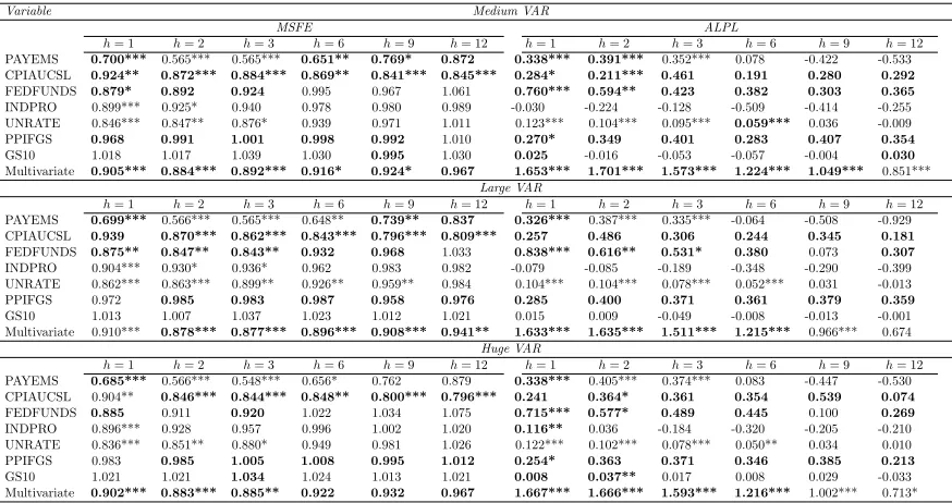
forecasting results for seven variables of interest: industrial production growth (INDPRO),

the unemployment rate (UNRATE), total nonfarm employment (PAYEMS), the change in

the Fed funds rate (FEDFUNDS), the change in the 10 year T-bill rate (GS10), the finished

good producer price inflation (PPIFGS) and consumer price inflation (CPIAUCSL).13 In

particular, we estimate VARs of different dimensions, with these seven variables included in

all of our specifications. We have a Medium VAR with 19 variables, a Large VAR with 46

variables and a Huge VAR with all 129 variables.14 A listing of all variables (including

which appear in which VAR) is given inAppendix A. Note that most of our variables have

substantial persistence in them and, accordingly, the first own lag in each equation almost

always has important explanatory power. Accordingly, we do not compress the first own lag.

This is included in every equation, with compression being done on the remaining

12_{In addition to dropping a few series with missing observations, we also remove the series non-borrowed}

reserves, as it became extremely volatile during the Great Recession.

13_{We also standardize our variables prior to estimation and forecasting. The forecasts of the original variables}

are then computed by inverting the transformation and reassigning means and variances. This standardization is computed recursively, i.e., using only the data that would have been available at each point in time to estimate the various models.

14

variables.15 Following Banbura et al. (2010), we choose a relatively large value for lag length

(p = 13) for all the methods we compare, trusting in the compression or shrinkage of the

various methods to remove unnecessary lags.

4.2 Estimating the Bayesian Compressed VAR

Random compression methods are most useful for forecasting and, hence, we will not discuss

estimation of the model’s parameters in any detail. However, before turning to forecasting, it

is worth presenting evidence relating to the random compression itself. This is controlled by

m and ϕ, which define the dimension and the degree of sparsity in the compression matrix.

Figure 1 and Figure 2 plot their empirical distributions for the Bayesian compressed VARs

of different dimensions. They can be interpreted as approximations to the posteriors of these

parameters. To aid in interpretation note that, in our compressed VARs, there is a different

compression matrix in each equation and so, for brevity, the figures average over all equations

and are based on the 75% of draws with highest posterior probability. Remember that smaller

values of m indicate a higher degree of compression and, for a given m, ϕ= 0.5 induces the

highest degree of sparsity.

The posteriors in the figures are clustered around sensible values. The high dimensional

data vectors,Z_ti, tend to be compressed down to dimensions of 10-20. The value ofm tends

to rise somewhat as we move from the Medium to Large to Huge VAR, but even for the latter

almost all the posterior weight if clustered below 20. It is also worth noting that, even though

we are drawing values ofmas low as 1, such draws never receive appreciable weight. In other

words, our algorithm is not attaching much weight to extreme compressions which reduce the

high-dimensional vector of predictors too much. The posterior for ϕ tends to be clustered

near the value which induces most sparsity.

4.3 Alternative Methods for Large VARs

We use the Bayesian compressed VAR methods introduced in section 3 in two ways: the

first one, which we label as BCVARc, compresses both the VAR coefficients and the error

15

covariances as in (9). The second one, which we label BCVAR, is the same, except for the

fact that it does not compress the error covariances.

To better assess the forecasting accuracy of these compressed VAR methods, we compare

their performances against a number of popular alternatives. Reasoning that previous work

with large numbers of dependent variables have typically used factor methods or large

Bayesian VARs, we focus on these. In addition, we compare the forecasts using all of these

methods to a benchmark approach which uses OLS forecasts from univariate AR(1) models.

Dynamic Factor Model

The dynamic factor model (DFM) can be written as:

Yt = λ0+λ1Ft+t

Ft = Φ1Ft−1+...+ ΦpFt−p+Ft (13)

whereFtis a q×1 vector factors (with qn) which contains information extracted from all

nvariables,λ0andλ1aren×1 andn×qmatrices, andt∼ N 0,ΣY

where ΣY is a diagonal

matrix. The vector of factors is assumed to follow a VAR(p) process with F_t ∼ N 0,ΣF,

with t independent of Fs at all t and s. We use principal component methods to estimate

the factors.16

We select the number of factorsqand the lag lengthpas follows: We specify the maximum

number of factors and lag lengths to beqmax=√nandpmax= 13, respectively. Next, at each

point in time we use BIC to choose the optimal lag length and number of factors. We use

Bayesian methods with non-informative priors to estimate and forecast with this model (note

that the law of motion for the common factors in equation (13) is needed to iterate forward

the forecasts whenh >1).

Factor-Augmented VAR

We use the Factor-Augmented VAR (FAVAR) of Bernanke, Boivin, Eliasz (2005) dividing

Ytinto a set of primary variables of interest, Yt∗ (these are the same key seven variables listed

16

above), and the remainderYe_t, and work with the model:

e

Yt = ΛFt+Yte (14)

Ft Y_t∗

= B0+B1

Ft−1

Yt−∗1

+...+Bp

Ft−p Y_t−p∗

+∗_t.

The vector (F_t0, Y_t∗0)0 is assumed to follow a VAR(p) process with Ye

t ∼ N

0,ΣYe

, ∗_t ∼

N(0,Σ∗), and t independent of ∗s at all t and s. As with the DFM model, we rely on

principal component methods to extract the factors Ft, and select the optimal number of

factors q and the lag length p using BIC. We use Bayesian methods with non-informative

priors to forecast with this model.

Bayesian VAR using the Minnesota Prior

We follow closely Banbura et al (2010)’s implementation of the Minnesota prior VAR which

involves a single prior shrinkage parameter, ω. However, we select ω in a different manner

than Banbura et al (2010), and estimate it in a data-based fashion similar to Giannone, Lenza

and Primiceri (2015). We choose a grid of values for the inverse of the shrinkage factor ω−1

ranging from 0.5×√npto 10×√np, in increments of 0.1×√np. At each point in time, we use

BIC to choose the optimal degree of shrinkage. All remaining specification and forecasting

choices are exactly the same as in Banbura et al (2010) and, hence, are not reported here. In

our empirical results, we use the acronym BVAR to refer to this approach.

To conclude this section, we would like to stress that we are only comparing our methods to

alternatives that are computationally feasible with large VARs. This rules out many popular

VAR-based approaches and explains why we are only considering the Minnesota prior VAR.

But we note that even the Minnesota prior VAR will not handle the truly enormous VARs that

may arise for the researcher working with multi-country data sets or combining macroeconomic

and financial data. Random compression methods should scale up to handle VARs with

thousands of variables (as will principal components methods), but the Minnesota prior VAR

will not. Carriero, Clark and Marcellino (2016a) explore in detail the computational challenges

of working with large VARs, and note that the posterior covariance matrix for the VAR is an

(np+ 1)nmatrix and manipulating this is the chief computational bottleneck. With general

approaches (which do not involve a natural conjugate or Minnesota prior) manipulating such a

matrix involvesO n6p3

(e.g. the Minnesota prior) this can be reduced to O n3p3. This is a huge computational

reduction whenn= 100 which explains why so many large VAR researchers use priors which

have this Kronecker structure (despite well known criticisms of it). But when n = 1000 or

n = 10,000 even if the Kronecker structure is maintained there will come a point where

computation will break down. Furthermore, when forecasting with large VARs the Minnesota

prior is mainly used for point forecasting since obtaining the predictive density typically

involves predictive simulation. This involves repeatedly simulating VAR coefficients and then

simulating future values of the variables. This raises additional computational bottlenecks

which limits the use of the Minnesota prior VAR in very large models.

4.4 Measures of Predictive Accuracy

We use the first half of the sample, January 1960–June 1987, to obtain initial parameter

estimates for all models, which are then used to predict outcomes from July 1987 (h = 1)

to June 1987 (h = 12). The next period, we include data for July 1987 in the estimation

sample, and use the resulting estimates to predict the outcomes from August 1987 to July

1988. We proceed recursively in this fashion until December 2014, thus generating a time

series of forecasts for each forecast horizonh, withh= 1, ...,12. Note that whenh >1, point

forecasts are iterated and predictive simulation is used to produce the predictive densities.

Next, for each of the seven key variables listed above we summarize the precision of the

h-step-ahead point forecasts for modeli, relative to that from the univariate AR(1), by means

of the ratio of MSFEs:

M SF Eijh =

Pt−h

τ=te2i,j,τ+h

Pt−h

τ=te2bcmk,j,τ+h

, (15)

where t and t denote the start and end of the out-of-sample period, and where e2

i,j,τ+h and

e2_bcmk,j,τ+h are the squared forecast errors of variable j at time τ and forecast horizon h

associated with modeli(i∈ {DF M, F AV AR, BV AR, BCV AR, BCV ARc}) and the AR(1)

model, respectively. The point forecasts used to compute the forecast errors are obtained by

averaging over the draws from the various models’ h-step-ahead predictive densities. Values

ofM SF Eijh below one suggest that modeliproduces more accurate point forecasts than the

AR(1) benchmark for variablej and forecast horizon h.

multivariate loss function of Christoffersen and Diebold (1998). Specifically, we compute the

ratio between the multivariate weighted mean squared forecast error (WMSFE) of model i

and the WMSFE of the benchmark AR(1) model as follows:

W M SF Eih=

Pt−h

τ=twei,τ+h

Pt−h

τ=twebcmk,τ+h

, (16)

where wei,τ+h =

e0_i,τ+h×W ×ei,τ+h

and webcmk,τ+h =

e0_bcmk,τ+h×W ×ebcmk,τ+h

are

timeτ+h weighted forecast errors of modeliand the benchmark model,ei,τ+h andebcmk,τ+h

are the (7×1) vector of forecast errors for the key series we focus on, and W is an (7×7)

matrix of weights. Following Carriero, Kapetanios and Marcellino (2011), we set the matrix

W to be a diagonal matrix featuring on the diagonal the inverse of the variances of the series

to be forecast.

As for the quality of the density forecasts, we follow Geweke and Amisano (2010) and

compute the average log predictive likelihood differential between model i and the AR(1)

benchmark,

ALP Lijh =

1 t−t−h+ 1

t−h

X

τ=t

(LP Li,j,τ+h−LP Lbcmk,j,τ+h), (17)

where LP Li,j,τ+h (LP Lbcmk,j,τ+h) denotes model i’s (benchmark’s) log predictive score of

variablej, computed at timeτ+h, i.e., the log of theh-step-ahead predictive density evaluated

at the outcome. Positive values ofALP Lijh indicate that for variable j and forecast horizon

hon average modeli produces more accurate density forecasts than the benchmark model.

Finally, we consider the multivariate average log predictive likelihood differentials between

modeliand the benchmark AR(1),

M V ALP Lih=

1 t−t−h+ 1

t−h

X

τ=t

(M V LP Li,τ+h−M V LP Lbcmk,τ+h), (18)

whereM V LP Li,τ+h and M V LP Lbcmk,τ+h denote the multivariate log predictive likelihoods

of modeliand the benchmark model at timeτ+h, computed under the assumption of joint

normality.

In order to test the statistical significance of differences in point and density forecasts, we

consider pairwise tests of equal predictive accuracy (henceforth, EPA; Diebold and Mariano,

conduct are based on a two sided test with the null hypothesis being the AR(1) benchmark.

We use standard normal critical values. Based on simulation evidence in Clark and McCracken

(2013), when computing the variance estimator which enters the test statistic we rely on

Newey and West (1987) standard errors, with truncation at lag h−1, and incorporate the

finite sample correction due to Harvey et al. (1997). In the tables, we use ***, ** and * to

denote results which are significant at the 1%, 5% and 10% levels, respectively, in favor of the

model listed at the top of each column.

4.5 Forecasting Results

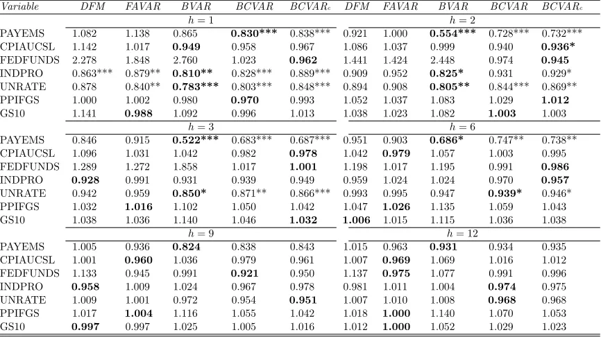
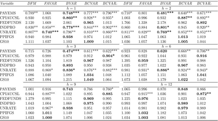
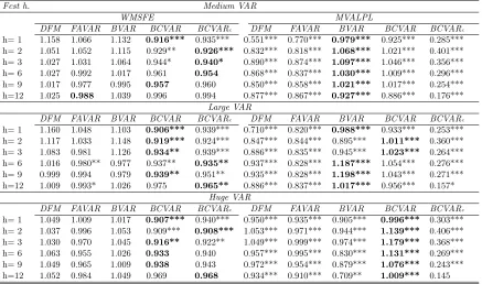
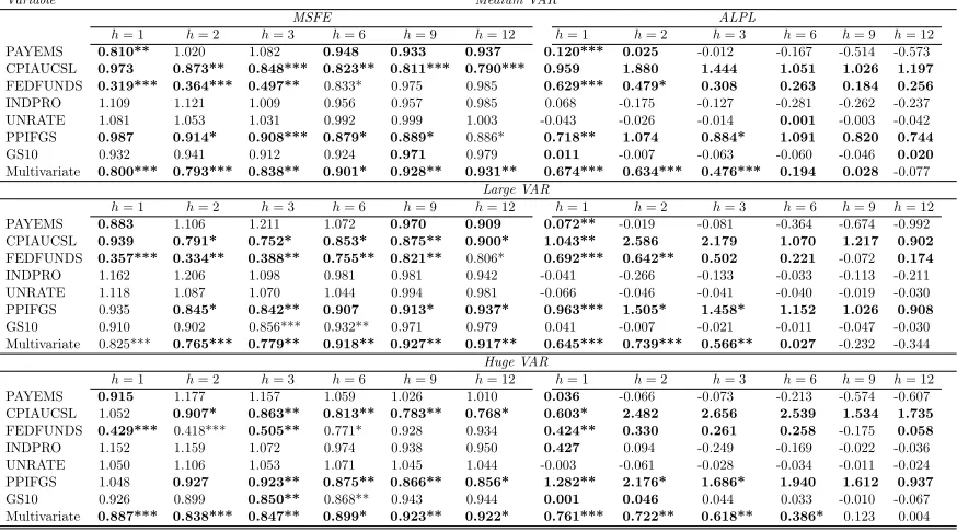
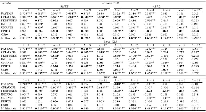
Tables 1 through 3 and the left side of Table 7 present evidence on the quality of our point

forecasts for our seven main variables of interest relative to the AR(1) benchmark. With a few

exceptions we are finding that BCVARs beat the benchmark and often tend to forecast better

than the other approaches. This holds, with several exceptions, for every VAR dimension,

variable and forecast horizon. Table 7, which presents the WMSFEs over the seven variables

of interest, provides the best overall summary of our results as they relate to point forecasts.

With six forecast horizons and three VAR dimensions, this table contains 18 dimensions in

which point forecasts can be compared. In 17 of these, either BCVAR or BCVARcis the model

with the lowest MSFE. In 12 of these cases, compressed VAR approaches beat the benchmark

in a statistically significant manner. The FAVAR is the next best approach, although it is

worth noting that in some cases (e.g. with short term forecasting and particularly with the

medium VAR) it does poorly, failing to beat the AR(1) benchmark. Overall, we are finding

random compression to work well, often the best but, in cases where it is not the best, it is not

too far from the best so that a risk averse user might feel confident using random compression

methods.

Thus, random compression of the VAR coefficients is at least competitive with other

multivariate forecasting methods with the data set under consideration. Evidence relating to

compression of the error covariance is more mixed. That is, in some instances the BCVARc

forecasts better than the BCVAR, but there are many cases where the forecasts from the

BCVAR model are more accurate.

for compressed VAR approaches to do particularly well at shorter horizons, but there are no

strong differences across horizons. In terms of the individual variables, one notable pattern in

these tables is that BCVAR and BCVARcare (with some exceptions) forecasting particularly

well for the most important macroeconomic aggregates such as prices, unemployment and

industrial production. In contrast, for the long-term interest rate (GS10), our Huge or Large

VAR methods are almost never beating the benchmark. But at least in this case, where

small models are forecasting well, it is reassuring to see that MSFEs obtained using random

compression methods are only slightly worse than the benchmark ones. This indicates that

random compression methods are finding that the GS10 equation in the Huge VAR is hugely

over-parametrized, but is successfully compressing the explanatory variables so as obtain

results that are nearly the same as those from parsimonious univariate models.

Figures 3 through 5 present evidence on when the forecasting gains of BCVARs relative

to the other approaches are achieved. These plot the cumulative sum of weighted forecasting

errors (jointly for the N = 7 variables of interest) for the benchmark AR(1) model minus

those for a competing approach, CSW F EDiht =

Pt−h

τ=t(webcmk,τ+h−wei,τ+h), for different

sized VAR sizes and different forecasting horizons. Positive values for this metric imply that

an approach is beating the benchmark. For short horizons, BCVAR is the only approach that

consistently beats the benchmark model, throughout the whole forecast period. All other

approaches accumulate more forecast errors over time compared to the simple AR(1). It is

particularly interesting that during the 2007-2009 crisis all multivariate methods seem to,

at least temporarily, improve over the univariate AR(1). However, towards the end of the

crisis, for all methods but the BCVAR relative forecast performance deteriorates abruptly.

For longer forecast horizons some of the alternative multivariate models perform fairly well

(e.g., ath= 12, the FAVAR ends up being the best model by a short margin). Nevertheless,

even at these horizons BCVAR remains consistently a reliable forecasting model.17

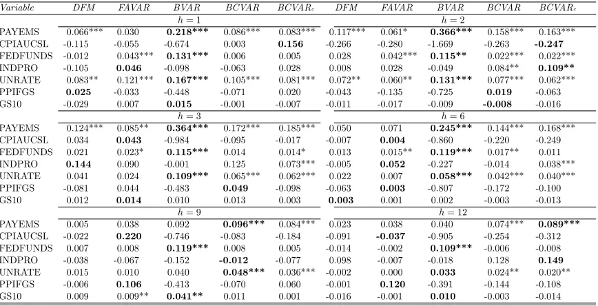
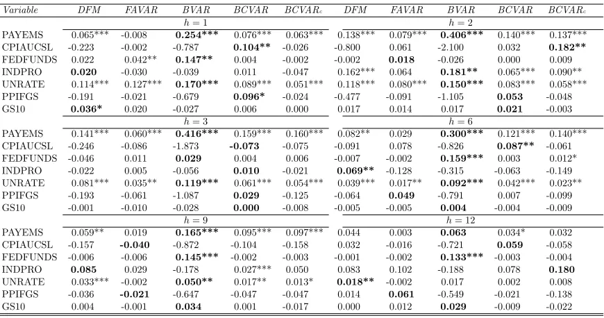
Tables 4 through 6 and the right hand side of Table 7 shed light on the quality of our

density forecasts by presenting averages of log predictive likelihoods for the VARs of different

dimensions. Results are similar as for MSFEs and we will not discuss them in detail. But they

17

do differ in their strength in two ways. First, the evidence that compressed VAR approaches

can beat univariate benchmarks becomes much more strong. See in particular the right hand

side ofTable 7which shows strong rejection of the hypothesis of EPA at every horizon and for

every VAR dimension. Second, the evidence that compressed VARs can forecast better than

BVAR or FAVAR approaches becomes somewhat weaker. In particular, with the medium and

large VARs standard large Bayesian VAR methods using the Minnesota prior tend to forecast

slightly better than the compressed VAR approaches. On the other hand, our BCVAR does

particularly well in the Huge VAR case, improving over the standard large Bayesian VAR and

FAVAR methods at all forecast horizons.

Figures 6,7 and 8 plot the cumulative sums of the multivariate log predictive likelihood

differentials, CSM V LP LDij = Pt−hτ=t(M V LP Li,τ+h−M V LP Lbcmk,τ+h), for VARs of

different dimensions and across a number of forecast horizons. It is interesting to note that,

in contrast to Figures 3 through 5, there is not strong evidence of a large deterioration in

forecasting performance relative to the univariate benchmark. In general, our compressed

VAR approaches may not be best in every case, but even when they are not they are close

to the best.18

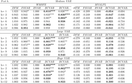
The preceding results compared the forecasting performance of various approaches to the

AR(1) benchmark. Tables such as Table 7 typically show strong evidence of statistically

significant improvements of all the multivariate forecasting methods relative to this

benchmark. To shed light on whether there are statistical significance differences between

the multivariate approaches, Table 8 presents forecast performance using the BVAR as the

benchmark. If we use log predictive likelihoods as the measure of forecast performance, it

can be seen that, although the compressed VAR approaches do better than the BVAR, this

difference is not statistically significant. In fact, there are not statistically significant

differences between any of our multivariate forecasting methods. When using MSFEs to

evaluate forecast performance there are, however, some cases where the compressed VARs

are forecasting significantly better than the Minnesota prior BVAR.

Finally, it is worth stressing that this section is simply comparing the forecast performance

18

of different plausible methods for a particular data set. However, the decision whether to use

compression methods should not be based solely on this forecasting comparison. In other,

larger applications, plausible alternatives to random compression such as the Minnesota prior

BVAR or any VAR approach which requires the use of MCMC methods, may simply be

computationally infeasible. The results presented in this section show that with the present

data set, random compression works fairly well. With larger data sets, it may very well be

that BCVAR is the only approach that is computationally feasible.

4.6 Robustness Checks

In the preceding sub-sections, we have shown that two particular ways of implementing

compression methods with VARs produce forecasts which are as good or better than more

computationally demanding alternatives. But there are many alternative ways of doing

random compression that we have experimented with. As noted previously a logical (and

simpler) way of doing random compression in VARs would be to use the natural conjugate

VAR of (5) instead of our equation by equation approach of (9). However, we have found

this to forecast very poorly. Other alternative approaches arise from different ways of

drawingϕ. We have tried several and found that they yield very similar results and, hence,

we will not discuss this issue further. Instead, in this sub-section, we present evidence on the

robustness of results to changes in ways the model averaging is done and to changes in the

way the variables are ordered.

Our main results use BIC-based weights to do model averaging (i.e. averaging over

different randomly drawn compressions). The BICs are calculated using the likelihood of the

entire vector of dependent variables, Yt. Given that we are only forecasting 7 key variables

of interest, we can also do model averaging using BICs only for these seven variables.

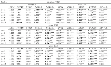
Table 9 (which is of the same format and should be compared toTable 7 ) summarizes the

forecasting performance for this approach. In a few cases, using BIC for only the 7 variables

of interest produces some very small improvements, but this makes very little difference.

To produce our main results, we ordered our dependent variables with our 7 variables

interest coming first. Our equation-by-equation approach to random compression implies

So it is possible that the way the variables are ordered will matter, especially when we are

compressing the error covariance matrix as in BCVARc. Table 10 presents results with the

7 variables of interest being ordered last (labelled BCVARc,v.2) compared to those of other

approaches. BCVARc and BCVARc,v.2 are producing very similar results.

5

Time-variation in Parameters: The Compressed TVP-SV

VAR

In macroeconomic forecasting applications, it is often empirically necessary to allow for

time-variation in the VAR coefficients and/or the error covariance matrix. There is an

increasing literature that shows that ignoring macroeconomic volatility and possible

structural changes in coefficients of a VAR can result in bad in-sample fit and poor

out-of-sample forecast performance; see for example Clark (2011). Both such extensions add

greatly to the computational burden since MCMC methods are usually required. In the

context of the constant coefficient VAR with conjugate prior for the VAR coefficients there

is a growing literature (e.g. Carriero, Clark and Marcellino, 2015, 2016a and Chan, 2015)

investigating various structures for time-varying error covariance matrices which do not lead

to excessively large computational demands. However, even these can be restrictive and

require the use of MCMC methods which will make them unsuitable for use in extremely

large models. Allowing for time-variation in the VAR coefficients (e.g. through assuming

coefficients evolve according to a random walk or a Markov switching process) will also

greatly increase the burden.

In this section, we show how the compressed VAR methods can be generalized to the

case of a VAR with time-varying parameters and stochastic volatilities (BCVARtvp−sv). Our

model becomes

Yi,t = Θci,t ΦiZti

+σi,tEi,t. (19)

Notice that relative to equation (9) now all parameters including the error variances may

vary over time and, thus, they havetsubscripts,t= 1, ..., T. We also remind the reader that

the variables Z_ti contain lags of the dependent variables and the terms which relate to the

error covariances as defined in (8). This TVP-SV VAR model is different from the previous

(2005) would specify the VAR in the familiar seemingly unrelated regression form, where all

n VAR equations are modeled jointly. Estimation using the latter form can become

cumbersome as n increases, since the posterior for both the time-varying regression

coefficients and volatilities involves many manipulations involving large data matrices.

Using (19), estimation of the BCVARtvp−sv is reduced to the estimation of n univariate

time-varying parameter regressions which is computationally more efficient for large n.

Additionally, the possibly large matrixZ_ti is still compressed using Φi as with the BCVAR.

In general, forecasting with TVP-SV VARs is computationally demanding as it typically

relies on MCMC methods. In our case, even if we use Φi to compress the data, a full Bayesian

analysis could be computationally demanding with largensince MCMC methods are required

and must be run for each of thenequations. Accordingly, we turn to approximate methods to

deal with the TVP-SV aspect of our BCVAR. These are generalizations of those developed by

Koop and Korobilis (2013) in the context of a time-varying parameter with time varying error

covariance matrix. They use variance discounting methods to model the time-variation in the

VAR coefficients and error covariance matrix, and provide analytical formulae for updating

them. Thus, in (19), once we draw Φi randomly, Θci,t and σi,t2 can be updated using simple

recursive formulae based on the Kalman filter, without relying on computationally intensive

MCMC methods.

Adapting Koop and Korobilis (2013), the compressed TVP-SV VAR model involves

estimating Θc_i,t and σ_i,t2 by assuming that they evolve according to:

Θc_i,t = Θc_i,t−1+ v u u t

(1−λi,t)var

Θc

i,t−1|t−1

λi,t

ui,t, (20)

σ_i,t2 = κi,tσ2i,t−1+ (1−κi,t)Eb_i,t2 . (21)

That is, Θc_i,t follows a random walk using a forgetting factor approximation to its error

covariance matrix. Kalman filtering methods can be used for this equation. Forσ2

i,t we have

an Exponentially Weighted Moving Average filter. Eb_i,t2 is the time t prediction error

estimated from the i-th equation of the VAR, ui,t ∼ N(0,1), and var

Θc_{i,t−1|t−1} is the

variance of Θc_i,t−1 given information up to time t−1 and is produced by the Kalman filter

the forgetting and decay factorsλi,t and κi,t. These factors, which are typically in the range

of (0.9,1), control how quickly discounting of past data occurs. For example, if λi,t = 0.90

then Θc

i,t depends very heavily on recent observations, and changes very rapidly over time.

On the other hand, ifλi,t = 0.99 the discounting of the past is more gradual and Θci,t varies

more smoothly. Finally, when λi,t = 1 we go back to the constant parameter VAR. Similar

arguments can be made forσ2_i,t and its decay factor κi,t.

For out-of-sample forecasting, we extend the methods of Koop and Korobilis (2013) by

allowing for the decay and forgetting factors to vary over time using simple updating formulae:

λi,t = λ+ (1−λ)×exp −0.5×

b E_i,t−2 ₁

b σ_i,t−2 ₁

!

, (22)

κi,t = κ+ (1−κ)×exp

−0.5×kurt

b

Ei,t−12:t−1

, (23)

whereσb 2

i,t−1 is the timet−1 estimate of the variance andkurt

b

Ei,t−12:t−1

is the kurtosis of

the VAR prediction error, evaluated over the past year (i.e. with monthly data this is based

on a rolling sample of 12 observations). λand κ put bounds on the minimum values of the

forgetting and decay factors. We setλ= 0.98 and κ= 0.94 which, in the context of monthly

data, allow for the possibility of a fairly large amount of time variation.19

Note that, if the prediction error is close to zero thenλit= 1 which is the value consistent

with the parameters in equation i being constant. In words, if the model forecast well last

month, we do not change its parameters this month. However, the larger the prediction error

is, the smaller λit becomes and, thus, a higher degree of parameter change is allowed for.

For the decay factor κi,t, we use a similar reasoning, except in terms of the kurtosis of the

prediction error. As is well known (e.g. from the GARCH literature), assuming that errors

are Normally distributed, in times of constant volatility kurtosis will be equal to zero, but in

times of increased volatility kurtosis is higher. Allowing forκitto depend on the kurtosis over

the past year is a simple way of allowingσi,t to change more rapidly in unstable times than

in stable times. Using these methods, it is straightforward to allow for time-variation in our

compressed VAR approach in a computationally simple manner.

19

Figure 9, which plots the time series of the predictive density volatilities for the Medium

BCVARtvp−sv against the time series of volatilities obtained from the alternative methods

described in section 4, confirms that heteroskedasticity plays a very important role in our

data. While the alternative methods allow for some time variation in the volatilities (they are

estimated on an expanding window of data), BCVARtvp−sv is finding a lot more variation.

This is particularly true at the time of the financial crisis.

Table 11, Figure 10, and Figure 11 present results on the forecast performance of our

BCVARtvp−sv approach. The story that jumps out is a strong one: adding time variation in

the parameters and volatilities leads to substantial improvements in forecast performance.

Conventional wisdom has it that allowing for time-variation (particularly in the error

covariance matrix) is particularly important for predictive density estimation. In a time of

fluctuating volatility, working with a homoskedastic model may not seriously affect point

forecasts, but may lead to poor estimates of higher predictive moments. This wisdom is

strongly reinforced by our results. The right panels of Table 11 show that in terms of

predictive likelihoods, the BCVARtvp−sv performs much better than our other compressed

VAR approaches, and better (with some exceptions) than standard large VAR and factor

methods. This is particularly true when focusing on the multivariate predictive performance

and short to medium forecast horizons. In addition, improvements relative to the univariate

benchmark (as indicated by the stars in the table) are almost always strongly statistically

significant. In terms of MSFEs, allowing for time variation in parameters leads to some

improvements, but these improvements are not as large as those we find with predictive

likelihoods. Again, the multivariate results are particularly strong, for all VAR sizes and

forecast horizons. In summary, the message conveyed by Table 11 is a particularly strong

one: BCVARtvp−sv is forecasting better than any other approach considered in this paper.

Figure 10 indicates that, with some exceptions, the reported success in terms of overall

point forecast accuracy of the BCVARtvp−sv relative to the alternative methods we considered

(namely, DFM, FAVAR, and BVAR) is not the result of any specific and short-lived episodes

but is instead built gradually throughout the forecast evaluation period, as indicated by

the increasing lines depicted in the figure. Interestingly, both at h = 1 and h = 12, the

notable around the time of the financial crisis, but are not confined to it. Figure 11provides a

similar analysis in terms of the overall density forecast accuracy of the BCVARtvp−sv model.

The left panels of the figure show that at h = 1 the previously reported forecast success of

the BCVARtvp−sv is once again built steadily throughout the forecast evaluation period. On

the other hand, the right panels of the figure, which focus onh= 12, show that while up until

the beginning of the last financial crisis the BCVARtvp−sv is forecasting more accurately than

all the alternatives, the 2007-2009 period has a strong negative impact on its density forecast

performance.

The preceding results use individual AR(1) forecasting models as the benchmark for

comparison. Table 12 uses the Minnesota prior BVAR as the benchmark. It can be seen

that many of the forecast improvements of BCVARtvp−sv over the BVAR are statistically

significant.

5.1 Robustness Checks

With our constant coefficient models, we presented robustness checks with respect to: i)

which variables were used to calculate the BICs used to construct weights attached to each

compression and with ii) whether the ordering of the variables mattered. Table 13andTable 14

repeat these robustness checks for TVP-SV versions of our approach. In both cases, forecasting

performance is very similar. There is a very slight forecast deterioration when the 7 variables

of interest are ordered last. But overall we are still finding a high degree of robustness.

Our compressed TVP-SV VAR allows for time-variation in both VAR coefficients and the

error covariance matrix. To investigate which of these is more important, Table 15presents

forecasting results for the model with both sorts of time variation (labelled BCVARtvp−sv

in the table) as well as those with only variation in the error covariance matrix (labelled

BCVARsv in the table). Comparing these two models in the table, it can be seen that

allowing for time variation in both does lead to some forecast improvements.

We also wish to compare our approaches to other fully Bayesian VAR approaches which

allow for time-variation in parameters. The difficulty of doing so is computational. These

approaches require the use of MCMC methods which makes them infeasible in large VARs.

be scaled up to large VARs due to the computational burden. D’Agostino, Gambetti and

Giannone (2013) carry out a forecast evaluation exercise using this model with three variables

and even this is very computationally demanding. One recent approach that shows promise

for larger VARs with stochastic volatility is that of Carriero, Clark and Marcellino (2016b).

But even their model cannot handle the really large VARs.20 However, we have carried out a

comparison of their approach to ours for the Medium VAR and a Small VAR involving only

the 7 variables of interest.21 The top two panels of Table 15 compares our BCVARtvp−sv

and BCVARsv approaches to the model of Carriero, Clark and Marcellino (2016b) (labelled

BVARccm). Results from the three approaches are roughly similar. For the Small VAR, their

model tends to forecast slightly better at short horizons than our BCVARsv. But in the

Medium VAR our compressed approaches tend to forecast better (particularly when forecast

performance is evaluated using WMSFE). Accordingly, we are finding an ability to forecast as

well or better than a sophisticated fully Bayesian VAR with stochastic volatility where such a

comparison is possible. But methods such as Carriero, Clark and Marcellino (2016b), which

require the use of MCMC methods, are still not at the stage of being suitable for forecasting

with hundreds of variables, much less than thousands of variables that would be possible with

random compression.

6

Conclusions

In this paper, we have drawn on ideas from the random projection literature to develop

methods suitable for use with large VARs. For such methods to be suitable, they must be

computationally simple, theoretically justifiable and empirically successful. We argue that the

BCVAR methods developed in this paper meet all these goals. In a substantial macroeconomic

application, involving VARs with up to 129 variables, we find BCVAR methods to be fast

and yield results which are at least as good as or better than competing approaches. And,

in contrast to the Minnesota prior BVAR, BCVAR methods can easily be scaled up to much

20

Carriero, Clark and Marcellino (2016b) do impulse response analysis in a VAR with 125 variables, but in their forecast evaluation never work with more than 20 variables. The results inTable 15for the Medium VAR took 25 hours to run on a PC using a modern Core i7 and 32Gb of RAM.

21_{For the autoregressive coefficients we use the asymmetric Minnesota prior with shrinkage hyperparameter}