System Analysis and Robustness
Eugenio Moggi1, Amin Farjudian2, and Walid Taha3 1
DIBRIS, Genova Univ., Genova, Italy,[email protected] 2
Univ. of Nottingham Ningbo China,[email protected] 3
Halmstad Univ., Halmstad, Sweden,[email protected]
Abstract. Software is increasingly embedded in a variety of physical contexts. This imposes new requirements on tools that support the design and analysis of systems. For instance, modeling embedded and cyber-physical systems needs to blend discrete mathematics, which is suitable for modeling digital components, with continuous mathematics, used for modeling physical components. This blending of continuous and discrete creates challenges that are absent when the discrete or the continuous setting are considered in isolation. We consider robustness, that is, the ability of an analysis of a model to cope with small amounts of impreci-sion in the model. Formally, we identify analyses with monotonic maps between complete lattices (a mathematical framework used for abstract interpretation and static analysis) and define robustness for monotonic maps between complete lattices of closed subsets of a metric space.
Keywords: Analyses; Robustness; Domain theory.
1
Introduction
The following considerations are taken from the paper “Continuous modeling of real-time and hybrid systems: from concepts to tools” [12] by Berhard Steffen et al., which was published in a special section on timed and hybrid systems. They provide the context and motivations for the issues addressed in this short paper. 1. Having served as a successful paradigm in physics and engineering for more than 300 years, starting with the discovery of the differential calculus by Leibniz and Newton at the end of the seventeenth century,the continuous interpretation of time was overwhelmed by the digital revolution. 2. The key point of formal description techniques is their mathematical exact-ness: it is unambiguous how the specified system is going to behave. Exact-ness should, however, not be confused with precision: “the system must respond within at least 1 and up to 20 seconds” is exact, although one might argue that it is not precise. Exact specifications make the amount of imprecision explicit.
Imprecision. In a discrete setting one can achieve absolute precision4, in a con-tinuous setting there are two pervasive and unavoidable sources of imprecision:
1. imprecision in measurements, namely predictions based on a mathematical model and observations on a real system can be compared only up to the precision of instruments used for measurements on the real system, and 2. imprecision in representing continuous quantities in computer-assisted tools
for modeling and analyzing hybrid/continuous systems.
Thus, a real number x:Rin mathematics, becomesx±in physics, with >0
measurement error, in theory of computation becomes an interval [x, x] withx andxbelonging to a subset ofRwith exact finite representations (e.g., floating-point or rational numbers) [14]5. However, anyx:
R can beapproximated by
proper rational intervals[x, x] witharbitrarily small imprecision, i.e., for any δ >0 there are rational numbersxandxsuch thatx < x < xand 0< x−x < δ. Approximability extends to continuous maps onR. First, a continuous map f onRhas a Scott continuousnatural extension f(I)=M {f(x)|x:I} on the cpo IR of intervals ordered by reverse inclusion. Scott continuity implies that the imprecision of f(I) goes to 0 when the imprecision of I goes to 0. Second, f can be replaced by a Scott continuous F mapping proper rational intervals to proper rational intervals such thatF([x]) = [f(x)] =f([x]), thusf(I)⊆F(I). Whenf is not continuous, one must give up something. Namely, one can find a monotonicF onIRsuch that:
1. ∀x:R.F([x]) = [f(x)], butF fails to be Scott continuous, or
2. F is Scott continuous,∀I:IR.f(I)⊆F(I), but∀x:R.F([x]) = [f(x)] fails.
In both cases the property “F(I) converges tof(x) whenIconverges tox” fails.
Robustness. In [13], we introducedrobustness, a property of monotonic maps between complete lattices of (closed) subsets in metric spaces. Intuitively, ro-bustness requires that small changes to the input I of a map F cause small changes to its output, where the definition of small relies on the metrics. Often, analyses can be identified with monotonic maps between complete lattices. For instance, reachability analysis can be cast as a monotonic mapFon the complete lattice P(S) of subsets of the state space S, that takes a setI of initial states and outputs the setR(I) of states reachable fromI, thusI⊆R(I) =R2(I).
IfSis a metric space, then one has the mathematical framework to measure imprecision. The picture below shows the initial state s of three systems (red, green and blue) consisting of a ball that can move (in a one-dimensional space) under the effect of gravity. We assume that initially the speed is 0, thus froms onlysis reachable, i.e.,Rr({s}) =Rg({s}) =Rb({s}) ={s}, but:
4 This does not exclude the possibility of usingimprecise (aka loose) specifications. 5
– the red ball (top) is unstable, i.e., a small change s0 to s means thatRr({s0}) includes some states far from s;
– the green ball (middle) isstable, i.e., a small changes0 tos implies that all states inRg({s0}) are close tos;
– the blue ball (bottom) is stable, if a small changes0 affects
only the position (while the speed remains 0); it is unstable, if the speed can change (and there is no friction).
These claims onscan be recast as follows:Rg isrobust at {s},Rris not.
Background. We assume familiarity with metric/topological spaces, the notions of open/closed/compact subset of a space [4,10], and make limited use of Cate-gory Theory [2,3] and Domain Theory [8]. We may write x:X forx∈X.
– Every metric space is a topological space whose open subsets are given by unions of open ballsB(x, δ)=M {y|d(x, y)< δ}.
– O(S) is the set of open subsets of a metric/topological spaceS, C(S) is the set of closed subsets, andP(S) is the set of all subsets.
– P(S) is the complete lattice of all subsets ofS ordered by reverse inclusion, which is the naturalinformation order on over-approximations (thus, sups are given by intersections and infs by unions). Similarly,C(S) is the complete lattice of closed subsets ofS ordered by reverse inclusion (sups are given by intersections, but only finite infs are given by unions).
Contributions. The contributions of this short paper are:
1. A definition of imprecision in the context of metric spaces (Sec 2), related to thenoise model in [7] andδ-safety in [11]. The main point is that imprecision makes a subsetS of a metric spaceSindistinguishable from its closureS. 2. A notion of robustness [13] (Sec 3) for monotonic maps A:C(S1)→C(S2),
the restriction to closed subsets is due to indistinguishability ofS andS. 3. Results about existence of best robust approximations [13] (Sec 4).
2
Imprecision in Metric Spaces
Definition 1. Given a metric space S, with distance functiond, we define:
1. B(S, δ)=M {y|∃x:S.d(x, y)< δ}, whereS:P(S)andδ >0. Intuitively,B(S, δ)
is the set of points inSwith imprecision< δ.B(S, δ)is open, because it is the union of open ballsB(s, δ)withs:S, moreoverB(B(S, δ), δ0)⊆B(S, δ+δ0). 2. S:C(S)is theclosureofS:P(S), i.e., the smallestC:C(S)such thatS⊆C.
ForS:P(S)andδ >0the following holds:S⊆S⊆B(S, δ) =B(S, δ). Thus, in the presence of imprecision,S andS areindistinguishable.
3. Sδ=M B(S, δ)is theδ-fatteningofS:P(S). Intuitively,Sδ is the set of points
inS with imprecision≤δ. In fact,B(S, δ)⊆Sδ⊆B(S, δ0)when0< δ < δ0.
For S:P(S) the following holds: S = Tδ>0B(S, δ) =
T
δ>0Sδ. Thus, the
We consider some examples of metric spaces motivated by applications.
Example 1 (Discrete). A set S can be viewed as a discrete metric space, i.e., d(s, s0) = 1 whens6=s0. Any subsetSofSis closed and open. Thus,C(S) =P(S), and Sδ =S for δ≤1. More generally, if ∀s, s0:S.s6=s0 =⇒ δ≤d(s, s0), then ∀S:P(S).Sδ =S, i.e., an imprecision ≤δamounts to absolute precision.
Example 2 (Euclidean).Euclidean spaces Rn (and Banach spaces) are used for modeling continuous and hybrid systems [9]. For C:C(Rn), δ-fattening has a simpler alternative definition, namelyCδ ={y|∃x:C.d(x, y)≤δ}.
Example 3 (Products, sub-spaces, sums). The product S0×S1 of two metric spaces is the product of the underlying sets with metricd(x, y)= maxM
i:2 di(xi, yi). A subsetS0of
Sinherits the metric, thus can be considered a metric spaceS0. IfS0 is also closed, then C(S0)⊆C(S) and theδ-fattening ofS:P(S0) isSδ∩S0.
The sum`
i:ISi of anI-indexed family of metric spaces is{(i, x)|i:I∧x:Si} with metric d((i, x),(j, y)) = ifM i=j thendi(x, y) else 1. The following hold: P(`
i:ISi) ∼=
Q
i:IP(Si), i.e., a subset in the sum is a sum
`
i:ISi of subsets. Similarly, C(`
i:ISi)∼=
Q
i:IC(Si). Moreover, (
`
i:ISi)δ =
`
i:I(Si)δ forδ≤1.
Remark 1. Usually the state space of a hybrid automaton [1] is a (finite) sum of closed sub-spaces of Euclidean spaces. A hybrid system on a Euclidean space S is a pair H= (F, G) of relations onS. Equivalently,His a subsetF+Gof the metric spaceS2+
S2. Therefore, closure andδ-fattening are applicable to hybrid systems onS as well as to subsets ofS.
3
Analyses and Robustness
We identify analyses with arrows A:Po(X, Y) in the categoryPo of complete lattices and monotonic maps between them. The partial order≤allows to define over-approximations and compare them. We consider≤as an information order, thus:x0≤xmeans that x0 is an over-approximation ofx,x1≤x0 means that x1is a bigger over-approximation thanx0(hence, less informative).
The complete lattice⊥<>of truth values, usually denotedΣ, is isomorphic to P(1) with 1 being the singleton set{fail}, namely >(true) corresponds to∅ (cannot fail), while⊥(false) corresponds to{fail}(may fail). Safety analyses are arrowsA:Po(X, Σ), and over-approximations may give false negatives.
Example 4. Safety analysis for transition systems onScorresponds to the arrow Sf:Po(P(S2)×P(S)×P(S), Σ) such that Sf(R, I, B) = > ⇐⇒M R∗(I) and B are disjoint, i.e., the setR∗(I) of states reachable from the setI of initial states by (finitely many)R-transitions is disjoint from the setB of bad states.
C0ofC:C(S), i.e.,C⊆C0 (or equivalentlyC0 ≤C), we say that the imprecision ofC0 in over-approximatingC is≤δ ⇐⇒M C⊆C0 ⊆C
δ.
For a metric spaceS, there is an adjunction inPo (Galois connection) be-tweenP(S) andC(S). In particular, everyS:P(S) has abest over-approximation
S:C(S). In other words,C(S) is anabstract interpretation ofP(S) [5].
Definition 2 (Robustness [13]). Given A:Po(C(S1),C(S2))with S1 and S2
metric spaces, we say that:
– AisrobustatC ⇐⇒ ∀M >0.∃δ >0.A(Cδ)⊆A(C).
– Aisrobust ⇐⇒M A is robust at everyC.
Robustness is a trivial property of analyses in a discrete setting (Ex 1).
Proposition 1. If S1 is discrete, then everyA:Po(C(S1),C(S2))is robust. Most analyses are not cast in the right form to ask whether they are robust, but usually one can show that they have the right form up to isomorphisms inPo.
Example 5. We consider analyses for (topological) transition systems [6].
1. ReachabilityRfR:Po(P(S),P(S)) for a transition systemRonSis not a map on closed subsets, but can be replaced by the arrowC7→RfR(C) onC(S). This is the canonical way to turn arrows onP(S) into arrows onC(S), but it may fail to be idempotent. A better choice is thebest idempotent arrow on C(S) over-approximatingRfR, denotedRsRand calledsafe reachabilityin [13], i.e.,RsR(C)= the smallestM C0:C(S) such thatC⊆C0andR(C0)⊆C0. 2. Reachability Rf:Po(P(S2)×
P(S),P(S)) for transition systems on S. First, we replaceP(S2)×
P(S) with the isomorphicP(S2+S) (see Ex 3). Second, we proceed as done forRfR. In particular, we can replaceRf with safe reach-abilityRs:Po(C(S2)×
C(S),C(S)) for closed transition systems onS. 3. SafetySf:Po(P(S2)×P(S)×P(S), Σ) is definable in terms of reachabilityRf,
namelySf(R, I, B) ⇐⇒M Rf(R, I)#B, where # is the disjointness predicate. Any replacement forRf induces a corresponding notion of safety, e.g., safe safetySs:Po(C(S2)×
C(S)×C(S), Σ) isSs(R, I, B) ⇐⇒M Rs(R, I)#B.
Remark 2. An analysis A:Po(C(S1),C(S2)) is often robust at some C:C(S1), but it is rarely robust at everyC. For instance, letRC be the diagonal relation onC:C(R), which is a closed transition system onR, then
– RsRC is robust, since RsRC(I) =I for everyI:C(R); – Rs is robust at (RN, I) for every I:C(R), but
– Rs is not robust at (RR, I) when∅ ⊂I⊂R, becauseRs((RR)δ, I) =R.
Time automata are a special case of hybrid automata (e.g., see [12]), and the latter are subsumed by hybrid systems [9].Timed transition systemsare an abstraction for all these systems. In particular, there is an abstraction map α:Po(P(S2+
Example 6. Reachability is not appropriate when time matters. For a timed transition systemRonS, a better analysis isevolutionEfR:Po(P(S),P(T×S)), which gives the time at which a state is reached, namelyEfR(I)= the smallestM E:P(T×S) such that{0} ×I ⊆E and {(t+d, s0)|(t, s):E∧(d, s, s0):R} ⊆E. By analogy with reachability, one can defineEf:Po(P(T×S2)×
P(S),P(T×S)) and safe variantsEs:Po(C(T×S2)×
C(S),C(T×S)), and cast them in the form required by robustness. Safe evolution can be extended to include asymptotically reachable statesEs:Po(C(T×S2)×C(S),C(T×S)), whereTis [0,+∞].
4
Best Robust Approximations
Intuitively, when an analysisA:Po(C(S1),C(S2)) is robust atC,A(C) isuseful also in the presence of small amounts of imprecision. This is obvious for analyses A:Po(C(S1), Σ), where robustness atCmeansA(Cδ) =A(C) whenδissmall.
Definition 3. Given A:Po(C(S1),C(S2)), we say that:
– A0:Po(C(S1),C(S2))is a robust approximation ofA ⇐⇒M A0 is robust and ∀C.A0(C)≤A(C).
– A :Po(C(S1),C(S2))is abest robust approximation ofA ⇐⇒M
A is a robust approximation ofAsuch thatA0(C)≤A (C)for every robust approximationA0 ofA andC.
Every arrow has aworstrobust approximation, namely the mapC7→ ⊥, where⊥ is the least element inC(S2). There areA:Po(C([0,1]),C(R)) that do not have a best robust approximation (see [13, Ex 4.6]). WhenS1andS2are discrete metric spaces, everyA:Po(C(S1),C(S2)) is robust, thusA =A. We give conditions on metric spaces implying existence of best robust approximations. The first result applies to safety analyses and is related to the notion of robustness in [7, Def 2].
Theorem 1. IfS2 is a finite metric space, thenA:Po(C(S1),C(S2))has a best
robust approximationA given byA (C) =\{A(Cδ)|δ >0}.
Proof. C(S2) =P(S2)∼=Σn is a finite complete lattice, whenS2is a finite (and necessarily discrete) metric space withnpoints. Therefore,A0:Po(C(S1),C(S2)) robust atC means that there existsδ >0 such thatA0(C) =A0(C
δ).
Since{A(Cδ)|δ >0}is a chain in a finite lattice, there existsδ >0 such that A(Cδ0) =A(Cδ) whenδ0 < δ. Let δ(C) be the biggest element in (0,+∞] such thatA(Cδ0) =A(Cδ) whenδ0< δ < δ(C). DefineA (C)=M A(Cδ) forδ < δ(C), thenA is monotonic, sinceA (C) =A(Cδ)≤A(Cδ0)≤A (C0) when C≤C0 andδ < δ(C), andA is a robust approximation ofA, since
– A (C) =A(Cδ)≤A(C) whenδ < δ(C), and
– A (C) =A(Cδ) =A (Cδ0)[=A(Cδ0)] whenδ0< δ < δ(C).
H S0 s Sf Ss Sr SR
HE [0,1]
0 [0] Sf S0 S0 0< s≤1 [s,1] Sf Sf Sf
HD [0,1]
0 S0 S0 S0 S0 0< s≤1 (0, s] S0 S0 S0
HT {(x, y)|0≤x≤y≤1}
(0,1) S∗(0) Sf Sf Sf b= 0
(0,1) S∗(b)Sf]S(0)Ss Ss 0< b <1
(0,1) S(1) Sf Sf S0 b= 1
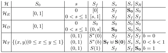
[image:7.612.163.454.115.208.2]ForHE andHD we takeH0= (F0, G0) withF0= [0,1]×[−1,1] andG0= [0,1]2. For HT = (F, G) we takeH0 = (F , G0) with G0 ={(y, y)|y: [0,1]} × {(0, y)|y: [0,1]}, and we use the notationS(b)= [0M , b]×[b] andS∗(b)=M ∪nS(bn) for subsets ofS0. The differences in the approximations of the reachable states are highlighted inbold. Table 1. Safe and robust over-approximations of the set of reachable states.
Theorem 2. IfS1 andS2are compact metric spaces, thenA:Po(C(S1),C(S2))
has a best robust approximationA given byA (C) =\{A(Cδ)|δ >0}.
Proof. We refer to [13] for details of the proof. The key points are:
– ifS is a compact metric space, thenC(S) is a continuous lattice;
– ifS1andS2are compact metric spaces, then a mapA0:Po(C(S1),C(S2)) is
robust exactly when it is Scott continuous. ut
5
Examples
We conclude by comparing different reachability analyses for threedeterministic
hybrid systemsH[9]:
HE a quantityx grows according to ODE ˙x = x when 0 ≤x < 1, and stays constant when it reaches the threshold 1, i.e., ˙x= 0 whenx= 1.
HD a quantityxdecreases according to ODE ˙x=−xwhen 0< x≤1, and it is
instantaneously reset to 1 when it is 0, i.e.,x+= 1 whenx= 0.
HT a timerxgrows while the timeout y stays constant, i.e., ˙x= 1& ˙y= 0 when 0≤x < y ≤1, when xreaches y it is reset and the timeout updated, i.e., x+= 0&y+=bywhen 0< x=y≤1 (withbconstant in the interval [0,1]), moreoverx+= 0&y+= 1 when 0 =x=y≤1, i.e.,y is reset to 1.
Table 1 gives for eachHabove (and initial states) the following sets:
– Sf =M RfH(s) set of states reachable (froms) in finitely many transitions,Sf is always a subset of the setS of the states reachable in finite time;
– Ss=M RsH(s) superset ofS computed by safe reachability;
– Sr=M RsH(s) superset ofSs robust w.r.t. over-approximations ofs;
Note that Sr depends on a compact subset S0 (over-approximating s and the
support of H), and SR depends also on a compact hybrid system H0 (with support S0 and over-approximating H). In particular,H0 constrains the over-approximations of H. The inclusions [s∈]Sf[⊆S] ⊆Ss⊆Sr ⊆SR[⊆S0] hold always. We explain why some of these inclusions are strict.
– H=HE &s= 0:Sf =S =Ss⊂Sr, because any small positive change to scauses the quantity to grow and eventually reach the threshold.
– H=HD &s >0:Sf =S ⊂Ss, because safe reachability includes 0, which is reachable only asymptotically (not in finite time), and any state inRfH(0). – H=HT &s= (0,1) & 0< b <1:Sf ⊂S =Ss, because the system has a
Zeno behaviour, namely the statex=y= 0 is reachable fromx=y = 1 in timeb/(1−b), but it requires infinitely many updates to the timeouty. Thus Sf computes an under-approximation of what is reachable in finite time.
– H=HT &s= (0,1) &b= 1:Sf =S=Sr⊂SR, because the imprecision inHδ means thaty can be updated with any value y+ in [max(0, y−δ), y] when 0< x=y≤1. Therefore,x=y= 0 is reachable inO(δ−1) transitions.
References
1. R. Alur, C. Courcoubetis, N. Halbwachs, T. A. Henzinger, P.-H. Ho, X. Nicollin, A. Olivero, J. Sifakis, and S. Yovine. The algorithmic analysis of hybrid systems. Theoretical computer science, 138(1):3–34, 1995.
2. A. Asperti and G. Longo. Categories, Types and Scructures: an Introduction to Category Theory for the working Computer Scientist. MIT Press, 1991.
3. S. Awodey. Category theory. Oxford University Press, 2010.
4. J. B. Conway. A Course in Functional Analysis. Springer, 2nd edition, 1990. 5. P. Cousot and R. Cousot. Abstract interpretation frameworks. Journal of logic
and computation, 2(4):511–547, 1992.
6. P. J. L. Cuijpers and M. A. Reniers. Topological (bi-) simulation.Electronic Notes in Theoretical Computer Science, 100:49–64, 2004.
7. M. Fr¨anzle. Analysis of hybrid systems: An ounce of realism can save an infinity of states. InComputer Science Logic, pages 126–139. Springer, 1999.
8. G. Gierz, K. H. Hofmann, K. Keimel, J. D. Lawson, M. W. Mislove, and D. S. Scott. Continuous Lattices and Domains, volume 93 ofEncycloedia of Mathematics and its Applications. Cambridge University Press, 2003.
9. R. Goebel, R. G. Sanfelice, and A. Teel. Hybrid dynamical systems. Control Systems, IEEE, 29(2):28–93, 2009.
10. J. L. Kelley. General topology. Springer, 1975.
11. S. Kong, S. Gao, W. Chen, and E. Clarke. dreach:δ-reachability analysis for hybrid systems. InInternational Conference on Tools and Algorithms for the Construction and Analysis of Systems, pages 200–205. Springer, 2015.
12. K. G. Larsen, B. Steffen, and C. Weise. Continuous modeling of real-time and hybrid systems: from concepts to tools. International Journal on Software Tools for Technology Transfer, 1(1-2):64–85, 1997.
13. E. Moggi, A. Farjudian, A. Duracz, and W. Taha. Safe & robust reachability analysis of hybrid systems.Theoretical Computer Science, 747C:75–99, 2018. Open access DOI 10.1016/j.tcs.2018.06.020.