Using Reinforcement Learning to Coordinate Better
Cora B. Excelente-Toledo∗
National Laboratory of Advanced Computer Science, LANIA R´ebsamen No. 80, Col. Isleta, C.P. 91090
Xalapa, Veracruz, MEXICO Tel. +52 228 8416100 ext. 5002
Fax. +52 228 8416101
Nicholas R. Jennings
School of Electronics and Computer Science University of Southampton
Southampton SO17 1BJ, UK. Tel. +44 23 8059 7681 Fax. +44 23 8059 3313
April 20, 2005
Abstract
This paper examines the potential and the impact of introducing learning capabilities into au-tonomous agents that make decisions at run-time about which mechanism to exploit in order to coordinate their activities. Specifically, our motivating hypothesis is that to deal with dynamic and unpredictable environments it is important to have agents that learn the right situations in which to attempt coordinationand the right coordination method to use in those situations. In particular, the efficacy of learning is evaluated when agents have varying types and amounts of information when those coordinating decisions are taken. This hypothesis is evaluated em-pirically, in a grid-world scenario in which a) an agent’s predictions about the other agents in the environment are approximately correct and b) an agent cannot correctly predict the others’ behaviour. The results presented show when, where and why learning is effective when it comes to making a decision about selecting a coordination mechanism.
Keywords: Coordination, agent interaction, collaborative agents, reinforcement learning.
1
Introduction
Effective coordination is essential if autonomous agents are to achieve their goals in a multiagent system (MAS). Such coordination is required to manage the various forms of dependency that naturally occur when the agents have inter-linked objectives, when they share a common environ-ment, or when they share resources. To this end, a variety of protocols and structures have been
∗This work was carried out while the first author was a member of the Intelligence, Agents, Multimedia Group at
developed to address the coordination problem. These range from long-term social laws (Shoham & Tennenholtz, 1992), through medium-term mechanisms such as Partial Global Planning (Durfee & Lesser, 1991), organizational structuring (Fox, 1981) and market protocols (Malone, 1987), to one-shot (short-term) mechanisms like the Contract-Net Protocol (Smith & Davis, 1981).
All of thesecoordination mechanismshave different properties and characteristics and are suited to different types of tasks and environments. They vary in the degree to which coordination is prescribed at design time, the amount of time and effort they require to set up a given coordination episode at run-time, and the degree to which they are likely to be successful and produce coordinated behaviour in a given situation. In the majority of cases, these dimensions act as forces in opposing directions; coordination mechanisms that are highly likely to succeed typically have high set up and maintenance costs, whereas mechanisms that have lower set up costs are also more likely to fail. Moreover, a coordination mechanism that works well in a reasonably static environment will often perform poorly in a dynamic and fast changing one. In short, there is no universally best coordination mechanism (Galbraith, 1973).
Given this situation, we believe it is important for the agents to have a variety of coordina-tion mechanisms, with varying properties, at their disposal so that they can select the particular mechanism that is most appropriate for the task at hand. Thus, for particularly important tasks, the agents may choose to adopt a coordination mechanism that is highly likely to succeed, but which will invariably have a correspondingly large set up cost. Whereas for less important tasks, a mechanism that is less likely to succeed, but which has lower set up costs, may be more appro-priate. However, to date, the choice of which coordination mechanism to use in a given situation is something that the designer typically imposes upon the system at design time (e.g. in a given application a particular social law will be used or it will be decided that all coordination activities will be handled by the contract net protocol). This means that in many cases the coordination mechanism that is employed is not ideally suited to the agents’ prevailing circumstances. This inflexibility means that the performance of both individual agents and the overall system may be compromised. This is especially the case in open and dynamic environments in which agent-based solutions are often deployed (Jennings, 2000).
To rectify this situation, our aim is to develop agents that can reason about the process of coordination and then select mechanisms that are appropriate to their current situation. That is, the choice of coordination mechanism is made at run-time by the agents that need to coordinate. We claim that fixing on a single coordination mechanism at design time is inappropriate, especially in dynamic and open contexts, because there is no scope for changing or modifying the mecha-nism to ensure there is a good fit with the prevailing circumstances (Bourne, Excelente-Toledo, & Jennings, 2000; Excelente-Toledo, 2003; Excelente-Toledo & Jennings, 2004). To circumvent this problem and to achieve the necessary degree of flexibility in coordination requires an agent to make decisions about when to coordinate and which coordination mechanism to use. To this end, we have previously developed, evaluated and shown the effectiveness of an agent reasoning frame-work to achieve this (Bourne et al., 2000; Excelente-Toledo, 2003; Excelente-Toledo & Jennings, 2004). However, this work also highlighted the importance (as well as the difficulty) of making good approximations about the behaviour of other agents. This is especially true as the environment becomes more dynamic. Given this, a natural extension of the framework is to enable the agents to acquire knowledge through run-time adaptation. Thus, the agents need to be capable of learning to make the right decisions about their coordination problem.
amount of information represented in the state varies. We show how this representation impacts upon the process of making run-time choices about the selection of coordination mechanisms in a number of different scenarios. The reason for this changing state representation is because it models the key determining factors of the agent’s reasoning framework (i.e. the environmental factors and the responses of the other agents in the group).
This work advances the state of the art in the following ways. Firstly, it introduces learning into that part of the agent’s decision making process that is concerned with when and how to coordinate (agents learn the right situations in which to attempt coordination and the right coor-dination method to use in those situations). Secondly, it explores different state representations inQ-learning implementation and, more importantly, it analyses the efficiency of each in different scenarios regarding coordination decisions. Finally, it empirically demonstrates where the benefits of learning can be obtained and where learning is not beneficial in this decision making context.
The remainder of this paper is structured as follows. Section 2 details our specific coordi-nation scenario. Section 3 introduces the decision procedures that enable autonomous agents to dynamically select coordination mechanisms. Section 4 explains how learning is applied to these decision making procedures. Section 5 introduces the experimental methodology used to perform a systematic empirical evaluation of the main hypotheses of this paper. Section 6 reports on the experimental work to evaluate the effect of introducing learning extensions into the agent’s de-cision making and examines their impact. Section 7 deals with related work and, finally, section 8 concludes and presents the areas of further work.
2
The Coordination Testbed
The testbed domain is described in more detail in (Bourneet al., 2000; Excelente-Toledo, 2003) (this includes a detailed justification for the choice of this scenario and the various design decisions within it). Here we just recount the basics that are necessary to understand the subsequent experiments. Our testbed consists of a grid world in which a number of autonomous agents (Ai) perform tasks
for which they receive units of reward (Ri). Each agent has a specific task (STi) which only it
can perform; there are other tasks which require several agents to perform them, calledcooperative tasks (CTs). Each task has a reward associated with it, the rewards for the CTs are higher than those for STs since they must be divided among them coordinating agents.
The agents move around the grid one step at a time, up, down, left or right, or stay still. At any one time, each agent has a single goal, either its ST or a CT over which coordination needs to be achieved. On arrival at a square containing its goal, the agent receives the associated reward. In the case of STs, a new one appears, randomly, somewhere in the grid, visible only to the appropriate agent. In the case of CTs, a new one appears, randomly, somewhere in the grid, but this is only visible to an agent who subsequently arrives at that square. If an agent encounters a CT, while pursuing its current goal (i.e., its ST), it takes charge of the CT1and must decide on both whether to initiate coordination with other agents over this task, and which coordination mechanism (CM) it should use or continue working on its ST. In this context, each agent has a predefined range of CMs at its disposal. Each CM is parameterised by two types of meta-data (see (Excelente-Toledo, 2003) for a mapping of several coordination mechanisms into this framework): set up cost (in terms of time-steps) and chance of success. For example, a CM may takettime-steps to set up (modelled by the agent waiting that number of time-steps before requesting bids from other agents) and have
1
a probability, p, of success (thus when the other agent(s) arrive at the CT square, the reward will be allocated with probability p, with zero reward otherwise). An agent may well decide that attempting to coordinate is not in its best interests, in which case it adopts the null CM (i.e. the agent rejects adopting the CT as its goal).
The Agent-in-Charge (AiC) of the coordination selects a CM and, after waiting for the set up period, broadcasts a request for other agents to engage in coordination. The other agents respond with bids composed of the amount of reward they would require in order to participate in the CT and how many time-steps away from the CT square they are situated. If an agent’s bid is successful, then it is termed Agent-in-Cooperation (AiCoop) to denote the fact that it is a participant (not AiC) for a CT task. If however, AiC initiates coordination but there is no AiCoops, then, we say that the AiC failed while attempting coordination. The role Agent-in-ST (AiS) is used to denote the situation where an agent is working towards a ST. Within this broad framework, Figure 1 highlights the specific decisions which have to be made (see Section 3 for more details) and gives the protocol the agents follow at each time-step.
[1] Agents arrive at a square. If AiS arrives at its ST cell, its goal is attained, it receives the reward and updates its goal. If AiCoop arrives at the CT cell, it notifies the AiC that it has arrived. The CT is achieved and the rewards are paid to AiCoops. Note that the reward is only given with probability p, the factor associated with the CM used to coordinate over the CT.
[2] If AiS finds a CT it must decide if it wants to become AiC and, if so, which CM= (t, p)it should use. Ift >0it must waitttime-steps before broadcasting a request for coordination. If AiC finds a new CT, it ignores it.
[3] If AiS receives a request for coordination, it decides whether and what to bid to participate in the CT. The AiC then evaluates all bids. If AiS’s bid is accepted, it adopts CT as its new goal. AiC does not respond to requests for coordination.
[4] Each agent decides on its next move according to its current goal and all agents move simultaneously.
Figure 1: Basic protocol followed by agents.
Agents might receive more than one proposal at the same time step, in which case they reply with as many bids as the proposals they receive. However, they will only accept one CT contract at a time. Agreements between AiCs and AiCoops to achieve a particular CT are established via a contracting protocol. This Contract-Net-like protocol (Smith & Davis, 1981) consists of three steps. In the first step, AiC broadcasts a proposal to all agents. It then waits for the bids. The second step involves selecting the bids and contracts from AiCs and AiS respectively (evaluation phase). Finally, the third step consists of the commitment about the terms of the contract and the time step at which AiCoops will arrive at the CT square.
variations is that they generate an environment in which agents face difficulty in estimating the decisions of other agents. Thus, agents have to make decisions based on factors that cannot be a priori predicted.
3
The Agent’s Decision Making Procedures
In our previous work we have developed and evaluated a decision making framework for reasoning about whether and how to coordinate in this domain (Bourneet al., 2000; Excelente-Toledo, 2003; Excelente-Toledo & Jennings, 2004). Since the main focus in this paper is on the role and impact of learning on this framework, we do not discuss all the details of the model here. Rather we concentrate on the decisions where learning could have a role to play; i.e. which CM to adopt, if any; how much to bid when a request for coordination is received; and how to determine which bid to accept, if any.
In this context, the agents’ aims are to maximise their reward; in particular their average reward per unit time. To this end, each agent keeps track of its own average reward, termed its reward rate, and it uses this rate to decide how much to charge for its own services and, occasionally, to approximate the expected rates of other agents (when it is not able to build up a picture of them). Specifically, each agent uses its reward rate to evaluate and compare the different actions available to it; if it can maintain or improve this rate, it chooses to do so. Of course, this decision model approximates the true relative values of different actions.
3.1 Deciding which CM to select
An agent which, while pursuing its current goal, encounters a CT must decide whether to initiate coordination with other agents in order to perform it. To do this, the agent must determine whether there is any advantage in so doing. This depends not only on the reward that is being offered, but also on the CMs available, as well as on various environmental factors which effect the expected demands of the potential coordinating agents.
To model the expected demands of the other agents, the AiC assumes they are randomly dis-tributed throughout the grid, and that their current goals are similarly disdis-tributed. Thus some agents may be near the CT while others may be far away; likewise, for some agents there would be a significant deviation from their ST to reach the CT, while others may be able to coordinate over the CT en route to their own goals. The agent then assesses the possible CMs on the basis of how long before the task can be performed and how much reward it is likely to obtain after deducting the expected reward requirement of the other agents. In the former case, it considers both the set up time and the average distance away each agent is situated, whereas the latter value is based on the amount of time agents must spend deviating to their path and the CM’s probability of success. This assessment determines the amount of surplus reward the agent can expect, over and above what it expects to obtain during its normal course of operation (i.e., its own average reward per time-step,r). The agent then selects the CM that maximises this surplus.2
To formalise this decision procedure, consider an [M×N] grid with reward size S for STs, and
R for CTs, a coordination mechanism, CMj = (tj, pj), which costst time-steps to set up and has
a probability of success p. In this grid world of known size, the agent can calculate the expected average distance (ave dist) away of any randomly situated agent from the CT square as well as the likely average deviation (ave dev) such agents would have to make to get there.
2
Based on these figures, the agent can assess the average surplus reward from coordinating over the CT at (x,y) using CMj = (tj, pj). First, it must estimate its own cost in terms of how long
the CM will take to set up and how long it expects to wait for the other agents to arrive. Since the AiC would usually expect to receiveS reward units per time-step, the average is calculated as
r= S
ave dist. The cost of CMj is then given by:
costj(x, y) =r×(tj+ave dist(x, y))
Second, the AiC must estimate the average amount of reward the other m agents will require. When AiC does not have any knowledge of the average reward of all the other agents in the environment, it uses its own (r) average reward as an approximation. 3
ave bidj(x, y) =m×
r×ave dev(x, y)
pj
(1)
Third, the AiC estimates the expected surplus (ave payoff) of CMj from adopting the CT by
taking into account the probability of success of the task:
ave payoffj(x, y) =pj×R
Using these estimates, the AiC can evaluate the expected surplus reward of adopting CMj:
ave surplusj(x, y) =ave payoffj(x, y)−costj(x, y) +ave bidj(x, y) (2)
When deciding which of its CMs to adopt, the agent computes its expected surplus reward from each of them and selects the one that maximises this value. If the surplus associated with all CMs is negative, the agent adopts the option of the null CM (which is defined to have zero surplus).
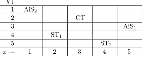
y ↓
1 AiS2
2 CT
3 AiS1
4 ST1
5 ST2
[image:6.595.190.428.448.542.2]x→ 1 2 3 4 5
Figure 2: Example of a coordination world grid.
To exemplify this decision procedure, consider the simple scenario of Figure 2 at one instant in time with two agents (AiS1and AiS2), two STs, one CT and two CMs: CM1(3,0.9) and CM2(6,1.0). AiS2 occupies a [5×5] grid and finds a CT requiring one other agent withR = 6 at square [3,2]. The average distance of other agents from [3,2] is 2.6. Since the average distance between two random squares is 3.2, the average deviation of any agent from [3,2] is 2. Assume that each ST has
3
a reward S = 2, then the average reward per time-step of all agents is 32.2 = 0.625. The expected surplus reward of adopting each CM is given by:
cost1(3,2) = (0.625×(3 + 2.6)) = 3.5
ave bid1(3,2) =
(0.625×1×2)
0.9 = 1.389
ave payoff1(3,2) = (0.9×6) = 5.4
ave surplus1(3,2) = 0.511
cost2(3,2) = (0.625×(6 + 2.6)) = 5.375
ave bid2(3,2) =
(0.625×1×2)
1.0 = 1.25
ave payoff2(3,2) = (1.0×6) = 6
ave surplus2(3,2) = −0.625
Under these circumstances, AiS2 decides to attempt coordination with CM1 (becoming AiC) because it expects to obtain a profit. Note this is not the case with CM2, where the negative result indicates there is not likely to be a surplus. Thus, in this case, if AiS2 only had CM2at its disposal it would choose the null CM (expected surplus zero) and it would continue towards its ST.
3.2 Deciding what to bid to become an AiCoop
When agents receive a request to participate in a CT they submit a bid based on the amount of reward that they would require to compensate them for deviating from their current goal. Thus, an agent’s required reward is determined by the amount of time spent in deviating to the CT square, its average reward per time-step and the probability of success of the CM being proposed. 4
To formalise this, consider an agent, Ai, with average reward per time-step ri. The agent
calculates its deviation (i.e., the number of extra time-steps it requires to reach its ST if it goes via the CT square). Note that if, for example, the CT square lies directly on a path to the ST, the agent’s deviation would be zero. Clearly, such an agent will be in a position to submit a very attractive bid, since the cost of coordinating is effectively zero.
Again by means of illustration consider the agents depicted in Figure 2. AiS1 at [5,3] would take 4 time-steps to reach ST1 at [2,4] directly, but 6 steps going via the CT at [3,2], a deviation of 2 time-steps. However, AiS2 at [1,1] would take 7 time-steps to reach ST2 at [4,5] directly, and also 7 steps going via the CT at [3,2]; AiS2 therefore has a deviation of 0.
To compute the reward AiSi requires from engaging in coordination over the CT, it takes into
account the compensation both for its deviation and for the possibility that the CM might fail. Thus, the estimation of bidby agent ito participate in coordination is given by:
bidij =
ri×deviationi
pj (3)
4
The agent submits its bid to coordinate and its distance from the CT square. If an agent is selected to coordinate, it adopts the CT as its current goal. Its ST is only re-adopted after the CT has been accomplished.
3.3 Deciding which AiS bids to accept
Once the AiC has received bids from all agents, it selects the set that maximises its surplus reward, given the new (definite) information it has received (cf. the approximation in section 3.1). For each agent, Ai, the AiC knows the amount of reward it will require (bidij) and the time it will take to
arrive (Ti).
The AiC’s selection bid process is based on the calculation of the cost of each bid received. However, when more than two agents are required to achieve a CT, it is necessary to deal with the fact that an AiCoop may have to wait in the CT cell while the remaining AiCoops arrive (because agents have to travel different distances). There are many ways of dealing with this situation (see discussion below). However to simplify the estimates of expected reward undertaken by the various agents, it is assumed the AiC pays an additional reward for the time elapsed. Thus, AiC knows the number of time steps that each AiCoop is likely to have to wait (specified in the bid) and the amount it will pay for waiting time at a specific predefined waiting rate (q). The CT is achieved only when the AiC has received the confirmation of allmagents involved in the cooperation. When an AiCoop notifies the AiC of its arrival at the CT cell, it either receives its share of the CT reward or the waiting rate followed by its share of the CT reward.
Thus, to decide which bids to accept, the general idea is that AiC selects them proposals with least cost (from the total bids receivedB). It does this by considering the reward requested in the bid and the waiting time cost (cost bid) and then it estimates its expected reward given this cost and its investment. Formally, AiC calculates the cost of each subsetbof Bwithm elements of the form (bidij, Ti). From each subset b, AiC selects the agent that will take the longest time to arrive
(i.e., maxTb = max(bidij,Ti)∈b[Ti]), then it can determine the maximum time that each agent will
spend in the cell. Finally, it approximates the cost of each bid based on the reward and the waiting time an AiC has to pay:
cost bidb =
X
(bidij,Ti)
(bidij + (maxTb−Ti)×q)
Bringing all this together, AiC estimates the surplus it expects to obtain by taking into account the cost of the selected bids and its own investment to wait for the last AiCoop to arrive. The bids selected belong to the subset bof Bthat maximizes the surplus given by:
surplusj =pj×R−cost bidb−r×(tj +maxTb) (4)
Now, it may be the case that no bids are received that give a positive surplus. Even though the chosen CM had an expected surplus, by chance it may be that no agents are sufficiently near to provide reasonable bids. In such a situation, the AiC abandons the CT and returns to its ST.
reasoning about coordination mechanisms (Bourneet al., 2000; Toledo, 2003; Excelente-Toledo & Jennings, 2004) and it is, therefore, the one we concentrate on in terms of evaluating the role of learning as described in the next Section. 5
4
The Role of Learning
Our investigation focuses on the use of reinforcement learning (RL) (Kaelbling, Littman, & Moore, 1996; Sutton & Barto, 1998) in coordination. A reinforcement-based approach is appropriate because we are concerned with agents pursuing goals and obtaining rewards according to how effectively those goals are accomplished. Within this class, Q-learning (Watkins & Dayan, 1992) was chosen because it is an online algorithm that does not require a model of the environment and thus it is well suited to our dynamic and unpredictable scenario.
In this study, each reinforcement learning agent uses a Q-learning algorithm. In general terms, an agent’s objective is to learn a decision policy that is determined by the state/action value function. The classical model ofQ-learning consists of:
• a finite setSof states sof the world (s∈S);
• a finite setAof actionsa that can be performed (a∈A);
• a reward function R:S×A→r.
An agent’s goal consists of learning a policy π : S → A that maximises the expected sum of discounted rewardsV:
V[rt+γrt+1+γ2rt+2+...] =V ∞ X
i=0
γirt+i
where 0 ≤ γ < 1 is the discount factor. Formally speaking, the discount factor determines the value of future rewards in the following way: a rewardrreceivedttime steps in the future is worth only γt times what it would be worth if it were received immediately. As γ approximates 1, the function takes future rewards into account more strongly. Thus, the agent’s task is to learn the optimal policyπ (i.e. arg maxπVπ(s),∀(s)).
In more detail, assume that an agent always performs the cycle of being in a particular states, then selecting and performing an actionathat causes the agent to enter a new state s′
and receive an immediate payoff (reward r(s,a)). The Q-learning algorithm is based on the estimated values of the agent’s state (s)-action (a) pairs, called Q(s,a) values. Based on this experience, the agent updates itsQ(s,a) values using the formula:
Q(s,a)←Q(s,a) +α[r+γ×max
a′ Q(s ′
,a′
)−Q(s,a)] (5)
whereαis the learning rate which determines the rate of change of the estimation and, maxa′Q(s′,a′) is the value of the action that maximises theQ function at states.
However, there is still the problem of how agents select their next action to execute. They have to balance their decision between selecting an action that, when exploited in the past, brought
5
about a positive reward, and an action that has not yet been explored and that consequently has an unknown reward (“exploitation versus exploration”) (Sutton & Barto, 1998). In this work, we use a ǫ-greedy function that selects the action with the highest Q(s,a) value once all the actions have been explored a pre-determined number of times. In particular, we use f(Q(s,a), n) (Russell & Norvig, 1995) which determines how greed (preference for high values of Q(s,a)) is traded off against curiosity (preference for low values ofn, namely, actions that have not been tried before). Formally speaking, the exploration function equates to:
f(Q(s,a), n) =
R+ ifn < Ne
Q(s,a) otherwise (6)
where n is the number of times Q(s,a) has been visited, R+ is the optimistic estimate of best possible reward that an agent can obtain in a given state and Ne corresponds to the number of
times that agents should try a particular action-state pair.
In summary, for experimental evaluation purposes, agents use a Q-learning algorithm with the following values: γ is assigned with value 0.01 which means that the agent is trying to maxi-mize immediate reward; α is decreasing with time by calculating it with the number of times a
Q(s,a) value is visited visits(s, a): α = 1+visits1 (s,a); the Q(s,a) values are initialised with 0. And equation (6) is used as the exploration function. 6
Thus, the main objective is then to evaluate the effect of learning on the agents’ decision making about CMs. To do this, we will compare the performance of agents that use aQ-learning algorithm (RL) with those that perform no learning (NL). Here the key difference is how the agents select the CM with which they will attempt coordination (step [2] in the protocol specified in Figure 1). For the remaining steps of the protocol, bothRLandNLagents employ the decision making procedures outlined in section 3 to make agreements when surplus (equation (4)) is positive given the set of
bids (equation (3)) it received.
This means then that when dealing withRLagents, the agent-state corresponds to the abstrac-tion of the particular situaabstrac-tion that agents experience when a CT is found (for example, the agent role and the position in the grid); the agent-action represents the set of options an agent has at its disposal (i.e. the set of coordination mechanisms it can select, including the null CM) and the reinforcement is modelled as the reward obtained by selecting the particular CM or not selecting a CM at all. Thus, the idea is that with Q-learning the agents will eventually learn the policy (after exploring sufficient situations) that allows them to know which CM to choose given a specific situation/state.
Now, for the purposes of this analysis, NL and RL agents experience one of the the following outcomes: i) a successful coordination (i.e. the AiC selects a CM, finds AiCoops to coordinate with and the CT is successfully achieved using the CM selected); ii) the AiC initiates coordination with a selected CM but there are not enough successful bids to make agreements (this means that attempting coordination with the CM was a failure); and iii) the AiC does not select any of the CMs at its disposal (i.e. the null CM is selected and the agent continues with its individual problem solving activity).
On the basis of previous description, the learning agent’s main objective is then to select the most suitable CM given its prevailing circumstances. To achieve this general goal, we explore the use of two Q-learning algorithms: RL1 and RL2. The main difference between them is in the way
6
they model the state representation at the moment when the decision about which CM to select is taken. In particular, our interest is in evaluating whether agents can improve their performance by explicitly representing one of the key components of the decision making of the CM, namely
the ave bid (equation (1)). 7 Thus, RL2 agents employ a Q-learning algorithm that does estimate
and use ave bid when selecting the CM, whereas RL1 does not model this information in its state representation.
Thus, in what follows, we first describe the generalRL algorithm and then we detail the differ-ences betweenRL1 and RL2. Finally, we discuss the algorithm followed by the NL agents.
RL: When a learning agent finds the CT, it performs the following basic cycle:
[1] It is in a particular state (represented by s)
[2] It makes a decision about the next action (a) to execute using the exploitation and exploration function of equation (6).
[3] The agent executes the selected action (a) which will be one of accomplishing a CT (if a CM is selected and successful), failing on a CT (if a CM is selected and unsuccessful), or selecting no CM (if the null CM is selected) and reaches a new states′
.
[4] It obtains a reinforcement reward as a result of the execution of action a. In particular, the reinforcement varies with the following outcomes:
• The CT is accomplished using the CM selected. In this case, a positive reinforcement is obtained that is based on the reward gained by achieving the CT after the payment to
theAiCoops and the time invested in pursuing the task.
• The CT failed given the CM chosen. This situation occurs because no one replies to the request for coordination or because the reward requested to participate in the cooperative action by theAiCoops is too high for the AiC to accept it (i.e. thesurplus(equation (4)) is negative). In either case, a negative reinforcement is calculated based on the average reward (r) lost in the time invested in the CM (t).
• The null CM is explored or exploited. Here, the reinforcement corresponds to the re-ward (CT rere-ward) the agent might have obtained by investing an average time in a CT (modelled by average distanceave dist).
[5] It updates the Q(s,a) value (equation (5)).
[6] It goes to [1].
Turning now to the differences between the learning agents and taking previous descriptions of
RL we have two variations: RL1 andRL2 agents. Each of them will be dealt in turn.
• RL1: An agent learns to select a CM by exactly following theRLalgorithm and, in particular, it uses its role and position in the grid when the CT is found as the representation ofs.
• RL2. An agent learns to select a CM usingave bid. An agent of this type followsRLbut has a modified state representationsand a different means of updating tos′in step [4]. Specifically,
7
s is modelled with the agent’s role, its position in the grid and the expected ave bid. 8 The initial estimation ofave bid in step [1] corresponds to:
ave bidj(x, y) =m×r×ave dev(x, y)
Note that the only difference between this formulation and equation (1), is that pj (the probability of success of a given CM) is unknown at this stage.
WhenRL2 agent reaches a new states′, the state is updated with theave bidusing equation (1) wherepj refers to the probability of success of the CM chosen.
NL: A non-learning agent makes decisions entirely based on the decision making procedures detailed in Section 3 and follows the protocol specified in Figure 1. Being precise, when an agent finds a CT, it calculates the expected average surplus (equation (2)) of each CM at its disposal. It then simply chooses the one with the bestave surplus. For the next stages of the protocol, it uses equations (4) to decide which bids to accept and (3) to becomeAiCoop. Note that theNLagent uses equation (1) to calculateave bid in order to evaluateave surplusfor each of the CMs.
To finish the discussion on the role of learning in this model, it is necessary to specify the features of the environment in which the algorithms will be tested. Two scenarios have been designed: scenario1 in which all AiSs in the environment become AiCoop by submitting a bid which is calculated by equation (3) and scenario2 in which AiSs calculate their bids in the same way but they vary the result by a random factor. The reason for this change is that, in the general case, AiCs face a great deal of uncertainty in predicting this value. Thus the random element mirrors environments in which predictions are less accurate. Together, these two scenarios constitute a reasonably static environment in which good predictions can be made and a more dynamic one in which predictions are inherently less accurate.
Bringing this all together, the agents’ performance will be analysed using the following algo-rithms:
RL1 agents learn to select a particular CM according to the profit gained by accomplishing CTs with a particular CM.
RL2 agents learn to select a particular CM according to the accuracy with which they calculate
theave bid.
NL agents select a particular CM using equation (2).
5
Evaluation Methodology
The main hypothesis we seek to evaluate is whether agents coordinate more effectively in our scenario using the reinforcement based algorithms. To measure such benefits in our model, a set of experiments have been designed as a formal methodology to provide information about the experimental variables. In order to test and to verify the hypothesis questions we employ statistical inference methods; in particular analysis of variance (ANOVA) is used to test hypotheses about differences between the means collected. The null hypothesis (H0) of equal means can be rejected when the procedure reveals for all experiments that the differences among means are significant
8
To simplify the state representation,ave bidis in fact associated with a range of values. Given the values of the simulation variables (see Section 5.1), the ranges of theave bidare the following: 1<ave bid<1.84, 1.84≥ave bid<
(p < 0.05) or might be accepted in the contrary case (Cohen, 1995). In other words, ANOVA tests the significance of the observations by accepting or rejecting the hypothesis formulated. The observations are the set of values for the experimental variables as the result of the execution of a particular algorithm in a given environment.
ANOVA explains the relationships between groups by analysing all possible interactions among them. However, though it provides an answer to the hypothetical questions by indicating if the mean of the groups are equal or not, it does not indicate the relations between them (for example, which mean of which groups are the highest). Thus, in most cases, it is necessary to go a step further (post-analysis) to determine where the exact differences among the means occur between groups. This procedure consists of running a post-test to explore the data collected on a case by case basis (this is termed pairwise analysis) because it tests the difference between each pair of means. 9 This pairwise analysis is particularly important in those cases where more than two procedures are being tested (or one procedure is tested in more than two scenarios). In concrete terms, the post-test makes a comparison between the data collected and builds groups (as many as necessary) that have statistically homogeneous values. Each group is generated with an associated value (the p value) that indicates the degree of confidence from which each group was built.
For the purposes of the experimental evaluation presented in Section 6, all the hypotheses are evaluated with ANOVA and only the cases that involve more than two experimental variables are subject to a post evaluation. When we test two variables and ANOVA rejects the equality of means, the data collected is used to indicate the relationship between the two variables. We are also interested in determining which of the groups obtains the highest mean (from now on referred to as thewinner group) because it represents the agents with the best performance.
5.1 Experimental and simulation variables
The following simulation variables were fixed for all learning experiments: size of the grid ([10×10]), duration (500,000 time units)10, number of CTs in the grid at any one time (3), number of agents in the environment (5), ST reward (1), CT reward (20), maximum number of agents needed to achieve a CT (3), coordination mechanisms considered by an agent (CM1= (1,0.6), CM2= (15,0.7), CM3= (30,0.8), CM4= (45,0.9) and CM5= (60,1.0))11.
The experimental variables on which the analysis is based are: total agent reward obtained from its ST and CT tasks (AU), total agent reward obtained by agents in the Agent-in-ST role (AiS), total agent reward obtained by agents in the Agent-in-Charge role (AiC), total agent reward obtained by agents in the Agent-in-Cooperation role (AiCoop) and, the total number of CTs accomplished (TCT). The experiments described collect the results of the experimental variables averaged over 10 simulation runs.
9
Several statistical tests exist to perform this analysis. The one used here is called Tukey’s honestly significant difference (HSD). This was chosen because it lies in the middle of the spectrum of alternatives; between LSD (which stands forleast significant differences) and Scheff´e tests which are the extreme in the conservative methods (Cohen, 1995; Lane, 2001).
10
We decided to evaluate over a fixed duration because in this scenario time counts and agents win reward at each time-step. Thus, it is reasonable to compare the behaviour of all algorithms under the same parameters. The duration selected is sufficient for the learning algorithms to converge to optimal values.
11
5.2 Evaluating hypotheses
To accept our main hypothesis, the hypotheses presented below must be rejected (meaning that the hypothesis of equal means is false) and the values of the experimental variables of a particular lear-ning algorithm should produce significantly better results than those obtained withNL. Therefore, the following hypotheses must be tested in scenario1 and scenario2:
H1: the AU obtained by performing a reinforcement based algorithm (RL) is the same as that obtained by agents which use the NL algorithm.
H2: the number of CTs (TCT) achieved by agents by means of either reinforcement learning algorithm is identical to that of agents using NL.
H3: theAUobtained byRL1 is the same as that of RL2 (evaluated in the case where H1 rejected).
H4: the number of CTs accomplished by RL1 is identical to that of RL2 (evaluated in the case where H2 is rejected).
6
Experimental Evaluation
[image:14.595.148.466.399.488.2]The experimental evaluation undertaken in this section follows the methodology described previ-ously and is organised in the following way. Firstly, the four hypotheses of Section 5.2 are tested in a static environment (Section 6.1) and secondly the same evaluation procedure is followed but in a dynamic environment (Section 6.2).
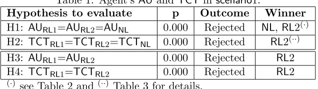
Table 1: Agent’sAU andTCT inscenario1.
Hypothesis to evaluate p Outcome Winner H1: AURL1=AURL2=AUNL 0.000 Rejected NL,RL2(·)
H2: TCTRL1=TCTRL2=TCTNL 0.000 Rejected RL2(··)
H3: AURL1=AURL2 0.000 Rejected RL2
H4: TCTRL1=TCTRL2 0.000 Rejected RL2
(·) see Table 2 and (··) Table 3 for details.
6.1 Selecting CMs in static environments (scenario1)
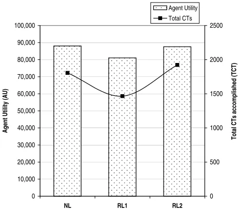
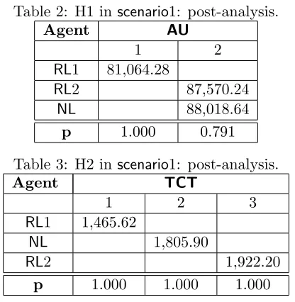
To start with, Table 1 and Figure 3 present a summary of the results obtained by performing ANOVA on the data collected by each of the algorithms in scenario1. Let’s first analyse the agent utility hypothesis. H1 is rejected, meaning that the performance of the algorithms does have a significant effect on the AU obtained. In order to understand the relationship between the algorithms a post-analysis of H1 is conducted (Table 2). The conclusion is that the performance of
NL andRL2 is better by a statistically significant amount (AUNL = 88,018.64,AURL2 = 87,570.24)
than RL1 (AURL1 = 81,064.28). Furthermore, comparing the performance of RL1 and RL2 in H3
(Rejected), it is concluded that the different mechanisms used for learning do effect theAUobtained by agents. Figure 3 graphically shows that the reward gained byRL2 agents is better than that for
RL1 agents. Moreover, it can also be concluded that an agent which learns to select the CM (RL2) performs the same as one which does not learn at all (NL).
0 10,000 20,000 30,000 40,000 50,000 60,000 70,000 80,000 90,000 100,000
NL RL1 RL2
[image:15.595.189.422.70.274.2]A g en t U ti lit y (A U ) 0 500 1000 1500 2000 2500 T o ta l C T s ac co m p lis h ed ( T C T ) Agent Utility Total CTs
Figure 3: Contrasting agent’s abilities in scenario1.
more CTs that are accomplished, the better the AU that is obtained. Here NL and RL2 agents accomplish more CTs thanRL1 and, consequently, they gain more reward (see axis Y of Figure 3 and the result of the post-analysis regardingTCTin Table 3). However, this is an important result to analyse in detail, because a high number of CTs achieved, does not necessarily mean that an agent performs better. This argument can be seen by observing Tables 2 and 3 (Figure 3 graphically shows the same information). Here, despite the fact that RL2 agents achieved statistically the highest number of TCT(three groups were formed in the post-analysis), theirAUgained is not higher than that obtained by NL agents (RL2 and NL agents belong to the same group in Table 2). Actually, the results of applying ANOVA to the TCT achieved and AU gained by NL and RL2 corroborate this explanation and are shown in Table 4. Specifically, H5 shows that the total reward obtained by RL2 is the same as that obtained by agents using the NLalgorithm (H5 is accepted, there is no statistically significant effect on the AU), whereas H6 demonstrates that the total number of CTs achieved by NL agents is identical to the TCTs accomplished by RL2 agents (H6 is rejected, the
TCTobtained by each algorithm is significantly different).
From the results obtained in the previous experiment it can be seen that in this scenario, the agent’s optimal behaviour is achieved by firstly taking the correct decision about when to attempt coordination. And, secondly, by selecting the CM whose time to set up is balanced by the amount of reward obtained. Moreover,RL2 andNLare the ones that make decisions which maximise their
AU. Thus, to better understand the differences or similarities between RL2 andNL, Table 5 tests ANOVA by agent role with the following hypotheses:
H7: theAUobtained by Agents-in-ST role which perform a reinforcement based algorithm (RL2) is the same as that obtained byAiS agents which use theNL algorithm.
H8: the total reward obtained by RL2 agents in the Agent-in-Charge role is the same as that obtained byNL AiC agents.
Table 2: H1 inscenario1: post-analysis.
Agent AU
1 2
RL1 81,064.28
RL2 87,570.24
NL 88,018.64
p 1.000 0.791
Table 3: H2 inscenario1: post-analysis.
Agent TCT
1 2 3
RL1 1,465.62
NL 1,805.90
RL2 1,922.20
p 1.000 1.000 1.000
Table 4: Contrasting RL2 and NLagents in scenario1. Hypothesis to evaluate p Outcome Winner
H5: AURL2=AUNL 0.594 Accepted none
H6: TCTRL2=TCTNL 0.000 Rejected RL2
Figure 4 illustrates these results. They indicates that while RL2AiCis significantly better than the corresponding NL agent role (H8 rejected), NL AiSis better than RL2 AiS (H7 rejected). H9 is accepted which means that the two agents accomplish similar rewards in theirAiCoop role. As can be seen, both agent types achieve (statistically speaking) the same AU (recall that H5 was accepted) but from different sources. In this experiment, the bestAiC(as a result of accomplishing more CTs) does not mean more reward is obtained. This is because highAUmight have originated from fewer and more profitable CTs (in the case of NL) or a high number of less rewarding tasks (in the case of RL2). In terms of selection of the CMs, this means that NL selected those with higher probability of success and higher time to set up (less time to achieve CTs), whileRL2 agents choose those CMs with less time to set up but less probability of success.
Table 5: Contrasting RL2 and NL agent’s roleAUinscenario1. Hypothesis to evaluate p Outcome Winner H7: AiSRL2=AiSNL 0.009 Rejected NL
H8: AiCRL2=AiCNL 0.000 Rejected RL2
H9: AiCoopRL2=AiCoopNL 0.546 Accepted none
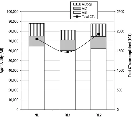
Whereas the previous discussion only comparedRL2 andNL agents, in what follows, we under-take a similar analysis but considering all three algorithms. To this end, Table 6 and Figure 4 show the result of the data collected and Tables 7, 8 and 9 present the post analysis performed to H10, H11 and H12 respectively.
H10: theAUobtained by Agents-in-ST role which perform a reinforcement based algorithm (either
0 10,000 20,000 30,000 40,000 50,000 60,000 70,000 80,000 90,000 100,000
NL RL1 RL2
[image:17.595.192.421.70.274.2]A g en t U ti lit y (A U ) 0 500 1000 1500 2000 2500 T o ta l C T s ac co m p lis h ed ( T C T ) AiCoop AiC AiS Total CTs
Figure 4: Contrasting agent’s roles abilities in scenario1.
H11: the total reward obtained byRL1 andRL2 agents in AiCrole is the same as that obtained by
NL AiC agents.
[image:17.595.126.488.424.495.2]H12: theAUobtained by RLs Agents-in-Cooperation role (AiCoop) is identical to the total reward obtained byNL agents in the AiCooprole.
Table 6: Agent’s roleAU inscenario1.
Hypothesis to evaluate p Outcome Winner
H10: AiSRL1=AiSRL2=AiSNL 0.000 Rejected NL(·)
H11: AiCRL1=AiCRL2=AiCNL 0.000 Rejected RL2(··)
H12: AiCoopRL1=AiCoopRL2=AiCoopNL 0.000 Rejected NL,RL2(···)
(·) see Table 7, (··) Table 8 and(···) Table 9 for details.
As expected, the first thing to notice is that the results are consistent with those described in Table 5. This is because NL and RL2 agents have superior performance in all three roles when compared against RL1 (H10, H11 and H12 are rejected). This means, the performance of RL1 agents do not have a significant effect on the experimental variables. NL still performs better than the others in terms of taking advantage of pursuing STs (i.e. by not attempting a cooperative activity (H10 rejected)). Turning to the analysis of the cooperative behaviour, here the results of Table 5 show thatRL2 is the agent which performs the best as anAiC (H11 is rejected) and (RL2 and NL) obtain the same as an AiCoop(H12 is rejected as both agents have statistically speaking the same results). Generally speaking, it can be seen thatRL2 andNLbetter balance their decision of when to go for the CT with the CM which allows them to gain more reward.
However, with RL2, agents additionally learn that this is the action to execute if and only if the
ave bid is higher than 2.64. Generally speaking, the optimal policy with RL2 might vary for each
[image:18.595.207.405.140.506.2]of the different values of theave bid, whereas withRL1 this information cannot be extracted from the policies because it is not explicitly represented.
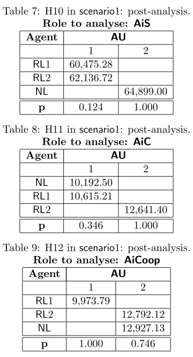
Table 7: H10 in scenario1: post-analysis. Role to analyse: AiS
Agent AU
1 2
RL1 60,475.28
RL2 62,136.72
NL 64,899.00
p 0.124 1.000
Table 8: H11 in scenario1: post-analysis. Role to analyse: AiC
Agent AU
1 2
NL 10,192.50
RL1 10,615.21
RL2 12,641.40
p 0.346 1.000
Table 9: H12 in scenario1: post-analysis. Role to analyse: AiCoop
Agent AU
1 2
RL1 9,973.79
RL2 12,792.12
NL 12,927.13
p 1.000 0.746
NLagents require knowing a priori what the regularities of the domain will be, whereas the learning agents can perform successfully as long as regularity exists. However, despite this improvement, we consider it very unlikely that agents will be able to take advantage of the knowledge learnt when the environment is in a constant state of flux. In such cases, it is not valid to assume that agents will continue behaving in similar ways or that the interaction will take place with the same agents they encountered before. In such scenarios, it will be more difficult to find NL agents that can accurately predict the other’s behaviour and it is very unlikely that agents can successfully use the same decision making framework. Thus, for these reasons, we believe our agents should be capable of adapting their decision making as a result of what is occurring in the environment, i.e. during acting in more demanding scenarios. Therefore, our objective is to design agents that inhabit open and dynamic environments and we require the learning agents to show a superior performance when considering both the exploring and the exploiting phases. Thus, in what follows, the use of learning is further explored in situations in which one of the fundamental actions associated with cooperative activity is more challenging to predict (scenario2).
6.2 Selecting CMs in dynamic environments (scenario2)
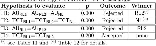
Turning now to the more dynamic environment of scenario2. We tested the same basic set of hypotheses (H1, H2, H3 and H4) and the results are summarised in Table 10 and Figure 5. First, we analyzed the hypotheses related withAU. Similar to the results obtained in Table 1, we conclude that applying RLs and NL produces distinctive results. But, conversely to Table 1,RL2 agents get significantly better results (AURL2 = 75,952.66) than RL1 agents (AURL1 = 73,690.06) and RL1
agents get a significantly higherAUthanNLagents (AUNL= 68,333.94). These results are clear in
[image:19.595.156.461.447.538.2]Figure 5 and the relationship between the groups is shown in Table 11. What is more, regarding the differences in the agents’ performances shown by the learning algorithms (H3), the results are once again that theAUof RL2 agents are significantly higher than those accomplished byRL1 agents.
Table 10: Agent’s AUandTCT inscenario2.
Hypothesis to evaluate p Outcome Winner H1: AURL1=AURL2=AUNL 0.000 Rejected RL2(·)
H2: TCTRL1=TCTRL2=TCTNL 0.000 Rejected NL(··)
H3: AURL1=AURL2 0.000 Rejected RL2
H4: TCTRL1=TCTRL2 0.200 Accepted none
(·) see Table 11 and(··) Table 12 for details.
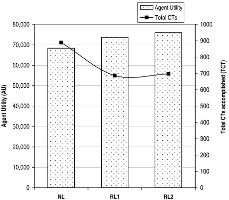
With reference to the TCT accomplished, the hypotheses of equal means of H2 and H4 are rejected. Figure 5 shows on its Y axis the total CTs accomplished by agent type. As can be seen, there is a significant impact on the TCTachieved when performingRL orNL; the results obtained by RLs are in the range of 30% less than those obtained by NL (Table 12 illustrates that after the post-analysis, RL agents accomplish (statistically speaking) the same number of CTs). The relevant aspect to discuss now, though, is that in contrast to previous experiments, NL obtains a lowerAUdespite achieving more CTs. This corroborates our previous explanation about the correct selection of the CM and its repercussions for the agent’s performance. To this end, Table 13 and Figure 6 show the results of testing ANOVA for the next hypotheses, as we did in scenario1:
H10: the total reward obtained by Agents-in-ST role which perform aRL algorithm (eitherRL1 or
0 10,000 20,000 30,000 40,000 50,000 60,000 70,000 80,000
NL RL1 RL2
[image:20.595.190.423.70.274.2]A g en t U ti lit y (A U ) 0 100 200 300 400 500 600 700 800 900 1000 T o ta l C T s ac co m p lis h ed ( T C T ) Agent Utility Total CTs
Figure 5: Contrasting agent’s abilities in scenario2.
H11: theAUobtained byRL1 andRL2 agents inAiCrole is the same as that obtained byNL AiCagents.
[image:20.595.200.416.400.610.2]H12: the AU obtained by RLs Agents-in-Cooperation role (AiCoop) is similat to the total reward obtained byNL agents in the AiCooprole.
Table 11: H1 in scenario2: post-analysis.
Agent AU
1 2 3
NL 68,333.94
RL1 73,690.06
RL2 75,952.66
p 1.000 1.000 1.000
Table 12: H2 in scenario2: post-analysis.
Agent TCT
1 2
RL1 686.54
RL2 697.46
NL 889.46
p 0.392 1.000
The results are as follows. The reward gained by achieving CTs by the cooperative roles NL
-AiCandNL-AiCoopare higher than those gained by the correspondingRLroles because they achieve
RLs. Thus, regarding the test of individual performance, H10 is rejected and RL2 is the agent type winner (Table 15 presents the distribution of the data collected regarding AiS roles). The reason for this result is that agents might invest a significant amount of time on the CM and, in the end, the AiCoops often request higher bids than those in scenario1 (meaning the AiCs’ profit is reduced). With NL, it seems that the AiCs cannot make good enough predictions of ave bid. Therefore they attempt coordination (or the AiC might even fail after the evaluation phase) even though the profit obtained after achieving the CT was not as high as the reward that was being gained by RL-AiSs. However, it is important to observe that the solution is not to avoid the CT tasks and only pursue STs in scenario2. Rather, the answer is to find the right balance between the two because in this scenario CTs always provide better rewards than STs. Thus, RL agents perform better because they are more certain about when to invest time in a CT with the correct CM and, more importantly, when not to do it (because it is not worth it). They then use this time to take advantage of pursuing STs.
0 10,000 20,000 30,000 40,000 50,000 60,000 70,000 80,000
NL RL1 RL2
[image:21.595.191.423.262.462.2]A g en t U ti lit y (A U ) 0 100 200 300 400 500 600 700 800 900 1000 T o ta l C T s ac co m p lis h ed ( T C T ) AiCoop AiC AiS Total CTs
Figure 6: Contrasting agent’s roles abilities in scenario2.
Table 13: Agent’s roleAU inscenario2.
Hypothesis to evaluate p Outcome Winner
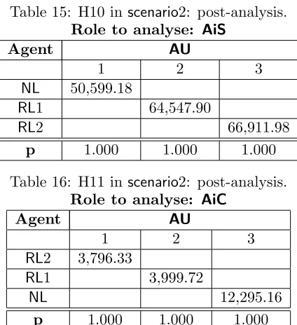
H10: AiSRL1=AiSRL2=AiSNL 0.000 Rejected RL2(·)
H11: AiCRL1=AiCRL2 =AiCNL 0.000 Rejected NL(·)
H12: AiCoopRL1=AiCoopRL2=AiCoopNL 0.000 Rejected NL(···)
(·) see Table 15, (··) see Table 16 and(···) Table 17 for details.
As this set of experiments shows, learning agents can take advantage of knowing which CM to apply in this more demanding environment. However, it is also important to evaluate how agents which employ the various reinforcement based algorithms compare with one another. To start with, the type of learning algorithms followed by the agents do not have a significant effect on the
[image:21.595.133.486.531.602.2]obtained per agent role indicates thatRL2 agents perform better thanRL1 in this environment. To this end, Table 14 shows the results of testing H13, H14 and H15 which read as follows:
H13: the total reward obtained byRL1AiSagents is the same as that obtained byAiSagents which use theRL2 algorithm.
H14: theAUobtained byRL1 andRL2 agents inAiC role is the same.
H15: the total reward obtained by RLs Agents-in-Cooperation role (AiCoop) is identical.
From the results of Table 14 it can be seen that the roles that have a significant effect on the
AUareAiCandAiS(H13 and H14 are rejected), whereas theAiCooprole does not make a significant difference to the final AUobtained (H15 is accepted). The explanation for this result is that RL2 agents are able to better balance their decision making about when to attempt coordination even though there is a significant degree of uncertainty about the outcome. This is achieved when an agent makes decisions about the CM based on the others’ cooperative behaviour (which is exactly what is being modelled by RL2). Thus, although at first it might seem a bad performance to accomplish more STs than any other agent type, when these results are combined with the results of the other roles, it is clear that RL2 agents show a better performance thanRL1. This is supported with the evidence that the biggest reward is gained byAiSagents and the reward gained by cooperative roles is the smallest amount.
Table 14: Agent’s roleAU inscenario2.
Hypothesis to evaluate p Outcome Winner H13: AiSRL1=AiSRL2 0.000 Rejected RL2
H14: AiCRL1=AiCRL2 0.000 Rejected RL1
[image:22.595.200.412.462.694.2]H15: AiCoopRL1=AiCoopRL2 0.400 Accepted None
Table 15: H10 in scenario2: post-analysis. Role to analyse: AiS
Agent AU
1 2 3
NL 50,599.18
RL1 64,547.90
RL2 66,911.98
p 1.000 1.000 1.000
Table 16: H11 in scenario2: post-analysis. Role to analyse: AiC
Agent AU
1 2 3
RL2 3,796.33
RL1 3,999.72
NL 12,295.16
In conclusion, it is not difficult to see that while in scenario1 the NL agents could accurately predict the amount requested from others for engaging in a CT, this was not the case for the more unpredictable environment of scenario2. As a result, agents might not only select an inappropriate CM, but they may also attempt coordination when this is not the best thing to do. Therefore, the optimal policy varies from attempting coordination less frequently than in a static environment to not attempting coordination at all. This is supported by the fact that the TCT gained by all agent types inscenario2 is considerably lower (TCThas a mean of 757.82) than the amount accom-plished inscenario1 (TCTmean of 1,738.24). Being more concrete, if theNL agents’ predictions of
ave surplus are too low (being optimistic about the possible future cooperative agents), they will
always initiate coordination even in situations where it not the best decision to make. However, if their predictions are too high (being pessimist) they will never attempt coordination. Thus, we can conclude that having learning agents that exploit and explore the CMs is the most reasonable thing to do in dynamic environments because agents cannot be certain about the others’ actions.
Generally speaking, in dynamic and unpredictable environmentsRLagents perform better than
[image:23.595.213.400.351.472.2]NLagents because they are more certain about when to invest time in a CT and, more importantly, when not to do it (because it is not worth it). RL agents then use this time to take advantage of pursuing STs. Moreover, incorporating theave bidin the learning process helpsRL2 agents to have a more precise model of what is occurring in the environment and, consequently, their decision making is improved. This, in turn, means the agents are more effective at maximising their profits.
Table 17: H12 in scenario2: post-analysis. Role to analyse: AiCoop
Agent AU
1 2
RL1 5,142.44
RL2 5,244.35
NL 5,439.59
p 0.060 1.000
7
Related Work
There are two broad strands of work that are primarily related to our model and each will now be dealt with in turn:
• work on reasoning about coordination and
• work on multiagent learning.
In more detail, Durfee (Durfee, 1999) has argued that agents need the flexibility to coordinate at different levels of abstraction, depending upon their particular needs at a given moment in time. To date, however, this work has focused on building such flexibility into the basic planning mechanisms of the individual agents. As yet, there are no mechanisms for explicitly reasoning about which level to coordinate at in a given situation. Such flexibility was also built into cooperative problem solving agents by Jennings (Jennings, 1993). Here, agents could choose to cooperate according to various conventions which dictated how they should behave in a particular team problem solving context. These conventions varied in terms of the time they took to establish and the communication overhead they imposed upon the agents. However, again, there was no reasoning mechanism for determining which convention was appropriate for a given situation. Barber et al. (Barber, Han, & Liu, 2000) present a software engineering framework that enables agents to vary their coordination mechanisms according to their prevailing circumstances. They also identify criteria for determining when particular mechanisms are appropriate. However, the decision procedures for actually trading-off these criteria are not well developed. Boutilier (Boutilier, 1999) presents a decision making framework, based on multi-agent Markov decision processes, that does reason about the state of a coordination mechanism. However, his work is concerned with optimal reasoning within the context of a given coordination mechanism, rather than actually reasoning about which mechanism to employ in a particular situation.
In terms of the work on learning, a vast literature has been produced in recent years concerning the use of learning techniques (particularlyQ-learning) in multiagent systems (Sen & Weiss, 1999; Stone & Veloso, 2000). The focus has been mainly on two aspects. In the first one, an agent’s goal is to learn about the other agents or their environment in order to predict their behaviour or to produce a model of them (Nagayuki, Ishii, & Doya, 2000; Hu & Wellman, 1998; Claus & Boutilier, 1998). Generally speaking, this strand of work deals with creating an explicit representation of other agents in order to predict their actions so that an agent can take more informed decisions in the future. In the second case,Q-learning has been applied to learn how to coordinate or cooperate to achieve common goals by using specific strategies (Tan, 1993; Sen, Sekaran, & Hale, 1994). The success in these two lines of research has mainly been to improve the cooperation or coordination between the agents in the environment. While this is clearly an important issue to address, we are more concerned with learning to select particular coordination mechanisms. To date, however, there has been comparatively little work concerned with learning which CM to select in a given context.
In our framework, agents are endowed with a set of decision making procedures to select ade-quate coordination mechanisms. By dealing with an abstract set of such mechanisms, we consider it more important to have agents that have the capacity to make decisions about coordination, rather than dealing with all problems might occur among the interactions specific interaction. We leave the latter to the details of the subsequent tasks of the associated protocol. Furthermore, we believe that as agents are increasingly being required to deal with more dynamic issues then online learning will become more important. COLLAGE, by contrast, uses instance based learning techniques in which there is a phase of recovery of examples and one of training. Consequently, the system has well defined moments in which these phases are performed which gives the additional problem of determining when each phase should finish.
In more recent research, Garland and Alterman (Garland & Alterman, 2001, 2004) propose the use case-based planning and learning probability estimates to allow agents to better coordinate. In particular, agents do learn on-line from past experience so that they take more informed decisions about which plan is “the” appropriate to execute in a particular coordination problem. In this work however, the learning outcome is to improve the decision making about planning, communication and adaptation of plans. This point of view is different from ours where it is assumed that planning is one instance of a CM and then the question to answer is whether planning should be selected in a specific circumstance.
In our previous reasearch work we have shown that autonomous agents that make run-time decisions about the most appropriate mechanism to coordinate their activities exhibit better per-formance than those that do not (Excelente-Toledo, 2003; Excelente-Toledo & Jennings, 2004). However, although the agents’ coordination decisions are more effective and efficient, as the envi-ronment becomes more dynamic and unpredictable, there is a greater need to exhibit behaviour that is tailored to the agents’ prevailing problem solving context. Thus, (Excelente-Toledo & Jen-nings, 2002) and (Excelente-Toledo & JenJen-nings, 2003) present a preliminary evaluation of how such flexibility can be achieved through learning and adaptation (specifically using Q-learning). How-ever this work does not deal with modelling others’ bids in the state representation and, moreover, it does not explore the effects of taking into account this key component of the agent’s decision making.
8
Conclusions and Future Work
This paper analysed the use and the efficacy of agents learning to make better decisions about how to coordinate more effectively. We showed that learning does indeed improve the decision making when agents are uncertain about the other agents’ actions. This improvement occurs because the agents learn to recognise the situations where the most profitable actions must be selected. We build upon (Excelente-Toledo & Jennings, 2002) to demonstrate that the more informed the decision making about the possible agents to coordinate with, the better the cooperative outcome. We also showed that learning was less effective when agents operate in more static environments in which they can make reasonably accurate predictions about their environment and other agents.
its components are in a continuous state of change (dynamism), or because the agents themselves exhibit different behaviour, have different capabilities and have their own agenda (heterogeneity). In these cases, it is especially important to have agents that are capable of automatically tailoring their coordination decisions to respond to the prevailing context. Examples of such systems are Web applications, e-commerce systems and grid computing application.
Speaking more generally, we believe it is important to develop techniques that enable agents to coordinate flexibly in dynamic and unpredictable environments. Although several of the detailed aspects of the decision procedures are specific to our grid-world scenario, we believe that the general processes and structures we developed are suitable for reasoning about coordination mechanisms in more general domains (see (Excelente-Toledo, 2003) for several examples of how the scenario can be mapped into a variety of real world problems including transportation problems and coordinated information retrieval) 12. In particular the issues of how to exploit learning techniques to allow agents to make decisions based on their experience is a key aspect that needs broader investigation. We believe that the results presented here among others can be viewed as an important first step in that direction.
For the future, the aim is to extend the use of learning to cover other aspects of the agent’s decision framework; such as to learn the decision about how much to bid in a request for coordination (Section 3.2), when to become an AiCoop (Section 3.1) and which bids to accept (Section 3.3). It is also intended to allow agents to construct models of one another and to have the ability to vary the details of this modelling according to the agent’s coordination context. In particular, it is believed that in order to accomplish more effective learning objectives, agents should model the others as 1-level agents(using the terminology of (Vidal & Durfee, 1997)) by explicitly representing knowledge about others or about the effect of their interactions. In this paper, we are addressing only part of the problem by assuming that the actions performed by other agents alter the environment that the agent is perceiving and sensing. Thus, agents do not explicitly model the behaviour of others. It is important to address this aspect because most of the agent’s decisions take into consideration predictions about the other agents and to refine these predictions an agent needs to represent in a more precise way the behaviour of the others in the scenario. In a broader context, a final aspect to discuss is that learning can also be employed to learn the meta-data parameters of the CM (i.e. the CM’s parameters could be refined given the efficiency of the CMs actual execution).
12
In (Excelente-Toledo, 2003) we mapped our grid world scenario into a package delivery problem (Rosenschein & Zlotkin, 1994) where trucks are the agents that move around the grid with parcels to deliver at specific locations. The final destinations for their parcels correspond to the agents’ specific tasks. There are special packages (a package being a group of parcels) that have to be delivered by more than one truck (because of their size) and these correspond to CTs. The truck’s goal is to deliver a number of parcels to specific locations. The more parcels delivered by a truck, the more profit it receives. Similarly, the coordinated information retrieval domain consists of having a number of agents with the task of downloading documents from specific locations in the Internet (Huhns & Stephens, 1999). The action of downloading has an associated cost that represents the price paid for the use of the server. The agent’s objective is to reduce, as far as possible, the cost of downloading. Each time an agent has a document to retrieve, it might download it by itself or it could minimise the cost by coordinating its activities with those of other agents that are also interested in the same document.