Maximum Likelihood with Auxiliary Information

M

AXIMUM

L

IKELIHOOD WITH

A

UXILIARY

I

NFORMATION

R

AY

C

HAMBERS

,

S

UOJIN

W

ANG

A

BSTRACT

Analysis of survey data does not happen in a vacuum. We typically know more about the target population than just the data observed in the survey. In some cases this extra information can be incorporated via calibration of survey weights. However, model fitting using weights often leads to increased standard errors. Also, weights are usually calibrated to a relatively small set of variables, while population data may be known for many more variables. Here we use the general approach to maximum likelihood estimation for complex surveys described in Breckling et al. (1994) to develop methods for efficiently incorporating external population information into model fitting using survey data. In particular, we focus on two simple, but very popular, models fitted to survey data. These are the linear regression model and the logistic regression model.

Maximum Likelihood With Auxiliary Information

Ray Chambers

Centre for Statistical and Survey Methodology, University of Wollongong

([email protected])

&

Suojin Wang

Department of Statistics, Texas A&M University

([email protected])

May 2005

Abstract

1. Introduction

Analysis of survey data does not happen in a vacuum. A model for the number of children ever born to a woman from a particular target population could depend on a number of factors, e.g. her age, her education level, her labour force status, her household income, her ethnic background and her access to family planning information, perhaps measured by presence or absence of a family planning clinic within a specified distance of her home. All of these variables are measured for women taking part in the survey, and the classical approach is to consider them ‘in isolation’ in the modelling process, implicitly assuming that the model fitted to these sample data is also appropriate for the population from which the sample is drawn. Sometimes, if this is felt to be too big an assumption, and survey weights are available, these are included in the model fitting process, assuming that they correct the parameter estimation process for potential sample selection bias.

However, we typically know a lot more about the target population than just the data observed in the survey. In particular we may know the total number of women in the population, their average number of children, their average age, their labour force participation rate and their ethnic distribution in the population. By ‘know’ here we mean either the actual population value or at least an accurate estimate. The question here is how to integrate this auxiliary population information into the model fitting process described above.

Second, weights are usually calibrated to a fixed and relatively small set of variables (e.g. age by sex population distributions, regional population distributions), while population data are often known for many more variables.

Alternative, more model-based, ways of incorporating auxiliary population information when modelling survey data have been explored in the econometrics literature, mainly in the context of analysis of linked data sets. An early example is Imbens and Lancaster (1994), who suggest a generalised method of moments approach to the problem of incorporating knowledge of the population expected value of the response variable Y into a sample-based linear regression of Y on an explanatory variable X. More recently, Qin (2000) has considered the same problem using a combination of empirical and parametric likelihood.

This paper focuses on developing methods for efficiently using auxiliary population information when survey data are used to fit a statistical model for a target population. In particular, we look at how maximum likelihood methods can be modified to incorporate this information. The approach we take is based on the general approach to maximum likelihood estimation for complex surveys described in Breckling et. al. (1994), hereafter referred to as BCDTW. In particular, we focus on two simple, but very popular, models fitted to survey data. These are the linear regression model and the linear logistic regression model.

2. MLE for a linear model given auxiliary population information

sample survey data to fit a simple normal linear model to the population values of Y and X. That is, we want to use the survey data to estimate the parameters α , β and σ2 that characterise the population model

σ_i−1

(y_i −α −βx_i) ~iid N(0,1) . (1)

Given this set-up, the maximum likelihood estimates (MLEs) for α, β and σ2 are

ˆ

β_smle= x_i(x_i−x_s)

s

∑

(

)

−1

x_i(y_i −y_s)

s

∑

ˆ

α_smle= y_s−βˆ_smlex_s

ˆ

σsmle

2 =

n−1 (yi−αˆols−βˆolsxi)

2

s

∑

.

We use a subscript of smle above to indicate that these MLEs are just based on the sample values of Y and X. However, suppose we also know the population mean y_U of Y. This can happen, for example, if the variable Y is also measured in a census, and census tabulations are published. In this case the OLS estimators above are no longer the MLEs forα, β and σ2. In order to obtain the ‘full information’ MLEs that include this additional information, we first observe that the population level score function for θ =(α,β,σ2) is defined by the components

sc1(θ)=σ

−2

(yi−α −βxi) U

∑

(2a)

sc₂(θ)=σ−2

x_i(y_i−α −βx_i) U

∑

(2b)

sc₃(θ)= −N / 2σ2 + (y_i −α −βx_i)2 U

∑

/ 2σ4. (2c)

these parameters. BCDTW show that this full information score function is the conditional expectation of the corresponding population level score function given these data. Denoting the components of this full information score function by an additional subscript of s, we have

sc_1s(θ)=σ−2 (E_s(y_i)−α −βx_i) U

∑

(3a)

sc2s(θ)=σ

−2

xi(Es(yi)−α −βxi) U

∑

(3b)

sc_3s(θ)= −N/ 2σ2 + (E_s(y_i)−α−βx_i)2 U

∑

+ Var_s(y_i) U

∑

⎡⎣ ⎤⎦/ 2σ4. (3c)

Since E_s(y_i)= y_i and Var_s(y_i)=0 for sampled population units, all we need to do is to determine these conditional moments for population units not in sample. To do this, we note that for non-sample unit i,

y_i

y_r xU ⎛ ⎝⎜

⎞ ⎠⎟ ~N

α+βx_i

α +βx_r ⎛

⎝⎜

⎞ ⎠⎟,

σ2

(N−n)−1σ2 (N−n)−1σ2 (N−n)−1σ2 ⎡ ⎣ ⎢ ⎤ ⎦ ⎥ ⎡ ⎣ ⎢ ⎢ ⎤ ⎦ ⎥ ⎥.

Here x_Udenotes the population values of X, y_r denotes the non-sample population average of Y and x_r denotes the corresponding non-sample average of X. Hence

y_i x_U,y_r ~N y⎡⎣ _r +β(x_i−x_r),σ2

(

1−(N −n)−1

)

⎤⎦. (4) Combining (3) and (4) leads to

sc_1s(θ)=σ−2

(y_i−α −βx_i) s

∑

+(N−n)(y_r −α−βx_r)

⎡⎣ ⎤⎦ (5a)

sc_2s(θ)=σ−2 x_i(y_i−α −βx_i) s

∑

+(N−n)x_r(y_r−α −βx_r)

⎡⎣ ⎤⎦ (5b)

sc_3s(θ)= −(n+1) / 2σ2+ (y_i−α−βx_i)2 s

∑

+(N −n)(y_r−α −βx_r)2

⎡⎣ ⎤⎦/ 2σ4. (5c)

ˆ

β_fimle =

∑

_sxi(yi−ys)+nxs(ys−yU)+(N−n)xr(yr−yU)

x_i(x_i −x_s)+nx_s(x_s−x_U)+(N −n)x_r(x_r−x_U)

s

∑

(6a)

ˆ

αfimle =yU −βˆfimlexU (6b)

ˆ

σfimle

2 =

(n+1)−1

(y_i −αˆ_fimle −βˆ_fimlex_i)2

s

∑

+(N−n)(y_r −αˆ_fimle−βˆ_fimlex_r)2

. (6c)

These estimators are identical to the estimators defined by a weighted least squares (WLS) fit to an extended sample consisting of the data values in s (each with weight equal to one) plus an additional data value (with weight equal to N – n) defined by the non-sample means yr and xr.

Intuitively, one expects the extra information from knowing y_U to contribute mainly to estimation of α in (1). To see that this is the case we now write down the variances of (6a) and (6b). This can be done by differentiating the score functions (5), changing signs and evaluating at the MLEs (6) to get the observed information matrix for these parameters. This matrix can then be inverted to get the (asymptotic) variances and covariances of these MLEs. Alternatively, exploiting their equivalence to a WLS fit, we can obtain the variances of the regression coefficients (6a) and (6b) directly. These are

Var( ˆαfimle)=n

−1σ2 xs

(2 )−

(1−nN−1

)(x_s(2 )−

x_r2 )

x_s(2 )−x_r2 +Nn−1(x_r2−x_U2)

⎛ ⎝⎜

⎞ ⎠⎟

Var( ˆβfimle)=

n−1σ2 xs

(2 )−

xr

2+

Nn−1(xr

2 −

xU

2

).

Here x_s(2 ) is the mean of the squares of the sample X-values. In an X-balanced sample (x_s = x_r = x_U) it is easy to see that Var( ˆβ_fimle) = Var( ˆβ_smle) while Var( ˆα_fimle)=Var( ˆα_smle)−n−1(1−nN−1)σ2, confirming our intuition above.

of view, the situation set out above is one where we have three calibration identities. We know the population size N, population total of X and the population total of Y. We could therefore calibrate the survey weights to recover these population totals. That is, if wi denotes the initial survey weight for sample unit i (e.g. the inverse of its sample inclusion probability), we replace this weight by w_i*, where w_i*

s

∑

= N, w_i*x_i s

∑

=N x_U and w_i*y_i s

∑

= N y_U. There are standard

methods for doing this (e.g. Deville and Särndal, 1992; Chambers, 1996). For simple random sampling, a least squares calibration criterion leads to weights w* =(wi

*

) , where

w*= N

n1n +N[1n ys xs] ′

1_n1_n 1′_ny_s 1′_nx_s ′

y_s1_n y′_sy_s y′_sx_s ′

x_s1_n x′_sy_s x′_sx_s ⎡ ⎣ ⎢ ⎢ ⎢ ⎤ ⎦ ⎥ ⎥ ⎥ −1 0 y_U −y_s x_U −x_s ⎛ ⎝ ⎜ ⎜ ⎞ ⎠ ⎟ ⎟.

Here 1n denotes an n-vector of ones, and ys, xsare vectors containing the sample values of Y and X respectively. The calibrated weights are then used to estimate α , β and σ2

by weighted least squares. That is, we estimate these parameters via

ˆ

βcalw = wi

*

xi(xi−xws) s

∑

(

)

−1

wi

*

xi(yi−yws) s

∑

(7a)

ˆ

α_calw= y_ws −βˆ_calwx_ws (7b)

ˆ

σ_calw2 =

N−1 w_i*(y_i −αˆ_calw−βˆ_calwx_i)2

s

∑

. (7c)

Here yws = wi

*

yi s

∑

/ wi

*

s

∑

=yU and xws = wi

*

xi s

∑

/ wi

*

s

∑

=xU.

described in Handcock, Rendall and Cheadle (2005), where the likelihood generated by the sample values of Y and X is maximised subject to this constraint. In the context of (1) this is the same as estimating α and β by minimising the sum of squared errors subject to this constraint. It is not difficult to see that this leads to the estimators

ˆ

βcon = (xi −xr)

2

s

∑

+n(xs −xU)

2

⎡⎣ ⎤⎦−1

(xi−xs)(yi−ys) s

∑

+n(xs −xU)(ys−yU)

⎡⎣ ⎤⎦ (8a)

ˆ

α_con =y_U −βˆ_conx_U (8b)

ˆ

σ_con2 =

n−1 (y_i −αˆ_con −βˆ_conx_i)2

s

∑

. (8c)

A slight generalisation of this approach (Li-Chun Zhang, private communication) is to maximise the sample-data likelihood subject to the predictive mean E y

(

_U |y_s,x_s,x_r

)

of y_U equalling its known value. This is equivalent to requiring that our estimates of α and β satisfy αˆ =yr −βˆxr. Maximising the sample-data likelihood subject to this constraint leads to estimators of the form

ˆ

βpred = (xi −xs)

2

s

∑

+n(xs−xr)

2

⎡⎣ ⎤⎦−1

(xi −xs)(yi −ys) s

∑

+n(xs −xr)(ys −yr)

⎡⎣ ⎤⎦ (9a)

ˆ

αpred =yr −βˆpredxr (9b)

ˆ

σ_pred2 =

n−1 (y_i−αˆ_pred −βˆ_predx_i)2

s

∑

. (9c)

In a balanced sample (x_s = x_r = x_U), ˆβ_fimle, βˆ_con and ˆβ_pred all reduce to the sample-based MLE

ˆ

β_smle and ˆα_fimle =αˆ_con. In general, the differences between the constraint-based estimators (8) and

(9) and the full information MLEs defined by (6) will be small.

BCDTW approach in this case then requires us to condition on this more limited information set, rather than on the information set assumed in the previous section. However, from (5) we see that the full information score functions in the complete X data case actually only depend on the non-sample X-values through their average x_r. This average is known given x_U and x_s. Using Result 2 of Chambers, Dorfman and Wang (1998) we conclude that the full information MLEs for this case (only x_U known) are also given by (6).

Suppose now that x_U is also unknown (so x_r is unknown). That is, the only population level data we have is the value of y_U. The formal BCDTW framework for calculating the MLEs of the parameters of (1) still applies in this ‘limited information’ case, however, and the component score functions (5) become

sc1s(θ)=σ

−2

(yi−α −βxi) s

∑

+(N−n)(yr −α−βEs(xr))

⎡⎣ ⎤⎦ (10a)

sc_2s(θ)=σ−2

∑

sxi(yi−α−βxi)+

(N−n)

{

Es(xr)(yr −α−βEs(xr))−βVars(xr)

}

⎡

⎣ ⎢ ⎢

⎤ ⎦ ⎥

⎥ (10b)

sc_3s(θ)= −n+1 2σ2 +

1 2σ4

(y_i−α −βx_i)2 s

∑

+

(N −n) (y_r −α−βE_s(x_r))2 +β2

Var_s(x_r)

{

}

⎡ ⎣ ⎢ ⎢

⎤ ⎦ ⎥

⎥ (10c)

where E_s(x_r) and Var_s(x_r) denote the expected value and variance of x_r conditional on the available data, i.e. the sample values of Y and X and the value y_r. The solutions to the estimating equations defined by (10) are then

ˆ

βlimmle =

x_i(y_i −y_s)

s

∑

+nx_s(y_s−y_U)+(N−n)E_s(x_r)(y_r −y_U)

xi(xi−xs)+nxs(xs −Es(xU))+(N−n)

{

Es(xr)(Es(xr)−Es(xU))+Vars(xr)

}

s

∑

(11a)

ˆ

ˆ

σ_limmle2 = (yi−αˆlimmle−

ˆ

β_limmlex_i)2

s

∑

+(N−n) (

{

y_r −αˆ_limmle−βˆ_limmleE_s(x_r))2+βˆ_limmle2 Var_s(x_r)

}

n+1 (11c)

where E_s(x_U)=N−1

[

nx_s+(N−n)E_s(x_r)

]

. Note that mutual independence of population units under (1) implies Es(xr)=E(xr |yr) and Vars(xr)=Var(xr |yr) . Assuming random sampling and a sample size n large enough to ensure that the joint distribution of yr, ys, xr and xs can be well approximated by multivariate normal distribution, we can then write down the approximations

E_s

( )

x_r ≈x_s +E x

(

_r −x_s|y_r −y_s

)

=x_s+βσ_x2

(

σ2+β2σ_x2

)

−1

(

y_r −y_s

)

(12) and

Var_s(x_r)≈(N−n)−1⎡_⎣σ_x2 −β2σ_x4

(

σ2 +β2σ_x2

)

−1⎤_⎦. (13) Here σ_x2

denotes the population marginal variance of X. Estimated values of E_s

( )

x_r and Var_s(x_r) can be calculated by substituting the sample-based estimates βˆ_smle and ˆσsmle

2

for β and σ2

, and the sample variance of X for σ_x2, in the right hand sides of (12) and (13). Substituting these estimates into (11) then leads to simple approximations to the maximum likelihood estimates for the parameters of (1) in this limited information situation.

Although there is no obvious extension of the prediction estimators (9) to where only population mean of Y is known, it is relatively easy to modify the calibration approach (7) for this case. Here there are two, rather than three, constraints defined by our knowledge of the population size (N) and the population mean of Y (y_U), and so the calibrated weights become

w_lim∗ = N

n1n +N[1n ys] ′

1_n1_n 1′_ny_s ′

y_s1_n y′_sy_s ⎡

⎣

⎢ ⎤

⎦ ⎥

−1

0 y_U−y_s ⎛

⎝⎜

⎞ ⎠⎟ .

estimators defined so far (with names given by their corresponding subscripts). The simulations are model-based, with population values first simulated, then sample values drawn from this population using simple random sampling without replacement (SRSWOR). A total of 1000 simulations were carried out for each scenario.

Not surprisingly, the results set out in Table 1 support our earlier comment that estimation of αshould benefit most from inclusion of the extra information about the population mean of Y. It is also clear that the full information MLEs (6) perform well (although their results are omitted, the constrained predictive estimators (9) were almost as efficient). With respect to RMSE, the estimators (7) based on full information calibrated weights are inefficient, even relative to the unconstrained sample-based MLEs that ignore the auxiliary information, while the limited information calibration and MLE estimators performed relatively poorly at small sample sizes. In the case of the MLE this was due to outlying estimates generated in a small number of samples where the estimation error for the population mean of X was large and negative. In the case of the calibration estimators this was due to negative weights being generated in these samples. A better assessment of the comparative efficiencies of the various estimators is therefore obtained by looking at their median absolute errors (MAE) in Table 1. Here we see a more consistent picture, with increased amounts of auxiliary population information leading to better inference, at least as far as α is concerned, with MLE-based methods that incorporate this inference clearly preferable.

substantial conditional bias, while the two limited information estimators also exhibit evidence of a conditional bias. This bias essentially disappears under full information ML estimation.

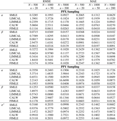
So far, our analysis has focussed on the improvement in efficiency that can be obtained when we include auxiliary information about the distribution of the model variables in the target population. Another advantage when this information is included, however, is that it can help protect inference from bias in cases where sample inclusion probabilities depend on these variables. To illustrate this, in Table 2 we report simulation results for the same scenarios explored in Table 1 but now where sample inclusion probabilities are either approximately proportional to X (PPX sampling) or approximately proportional to Y (PPY sampling).

The gains from using the full information MLEs under both PPX and PPY sampling are clear in Table 2. In contrast, the calibration-based estimators LIMCAL and CALW become quite unstable. The limited information MLE (LIMMLE) performs comparably with the sample-based MLE (SMLE) under PPX sampling, but is superior under PPY sampling. Although we do not show it here, the conditional bias properties of the different estimators of α under PPX and PPY sampling are qualitatively similar to those under SRSWOR (see Figure 1). In particular, the sample-based MLE is clearly conditionally biased, particularly under PPY sampling, while the limited information MLE has reduced conditional bias. The full information MLE of this parameter has essentially zero conditional bias.

3. MLE for a linear logistic model given auxiliary population information

wish to combine the sample data and this auxiliary information in order to model the relationship between Y and X in the population using a linear logistic model. For simplicity we assume independent population elements and simple random sampling.

For population element i, put π(x_i)=Pr(y_i =1 |x_i)=exp(α +βx_i) 1

(

+exp(α+βx_i)

)

−1. The population level component score functions for θ =(α,β) are then

sc₁(θ)= (y_i−π(x_i)) U

∑

sc₂(θ)= x_i(y_i−π(x_i)) U

∑

so the full information component score functions become sc_1s(θ)= y_i

U

∑

− π(x_i) U

∑

(14a)

sc_2s(θ)= x_i(y_i −π(x_i))

s

∑

+E_s

(

∑

_rxiyi

)

−

∑

_rxiπ(xi). (14b)

For arbitrary non-sample population element i, let r(i) denote the remaining N – n – 1 non-sampled population elements. Without loss of generality we assume t_ry >0 , so the conditional expectation in (14b) can be written

E y_ix_i r

∑

| y_i r

∑

=t_ry,x_r

(

)

= x_iE y_i | y_j

r

∑

=t_ry,x_r

(

)

r

∑

=

∑

_rxiPr

(

yi =1 |

∑

_ryj =try,xr

)

=

∑

_rxiPr

(

yi =1,

∑

_r(i)yj =try−1 |xr

)

Pr y_j

r

∑

=t_ry|x_r

(

)

= x_iπ(x_i)R_1i r

∑

where R1i =

(

Pr

(

∑

_ryj =try|xr

)

)

−1

Pr y_j r(i)

∑

=t_ry−1 |x_r(i)

(

)

. The full information score function

components defined by (14) are therefore sc_1s(θ)= (y_i −π(x_i))

U

sc_2s(θ)= x_i(y_i −π(x_i)) s

∑

− x_iπ(x_i)(1−R_1i) r

∑

. (15b)

A saddlepoint approximation to the second term on the right hand side of (15b) is developed in the Appendix. This is

sc_2s(θ)≈ x_i

(

y_i−π(x_i)

)

s

∑

− x_iπ(x_i) 1

(

−[1+(1−π(x_i)){b(t_ry)−1}]−1

)

r

∑

(15c)

with b(try)=exp ⎡⎣

∑

_rπ(xj) 1

(

−π(xj)

)

⎤⎦

−1

π(xj) r

∑

−try

⎡⎣ ⎤⎦

{

}

.

As noted already in section 2, it is extremely unlikely in practice that the actual non-sample X values will be known. Since the full information score function (15) depends directly on these values, we need to revise this function when non-sample X values are unavailable. In general, the score function for α and β is then defined by

sc_1s(θ)= y_i

U

∑

− π(x_i)

s

∑

−E_s

(

∑

_rπ(xi)

)

(16a)

sc2s(θ)=

∑

_sxi(yi −π(xi))+Es

(

∑

_rxiyi

)

−Es

(

∑

_rxiπ(xi)

)

(16b) where E_s denotes expectation after conditioning on the actual auxiliary information that we have (we continue to assume that t_ry is known). Suppose we know the non-sample mean x_r of X. We can then

approximate the conditional expectations Es

(

∑

_rπ(xi)

)

and Es

(

∑

_rxiπ(xi)

)

using a smearing approach (Duan, 1983). This is based on the assumption that, for an arbitrary function f of x that depends on some parameter θ, we can write

1

N−n

∑

r f(xi,θ)= 1

N −n

∑

rf x

(

r+(xi−xr),θ

)

≈ 1

n

∑

s f x

(

r −xs +xi,θ

)

. Put Δ =x_r −x_s. The smearing approximation to E_s π(x_i)

r

∑

(

)

is then

E_s

(

∑

_rπ(xi)

)

≈ N−n

We therefore replace the score component (16a) by sc_1smear(θ)= y_i

U

∑

− π(x_i) s

∑

− N−n

n

∑

sπ(Δ +xi). (17a)

A corresponding smearing approximation to (16b) that includes a saddlepoint approximation is given by (A.7) in the Appendix. This allows us to replace this component score by

sc_2smear(θ)= x_i

(

y_i −π(x_i)

)

s

∑

− N−n

n ⎛

⎝⎜ ⎞⎠⎟

∑

_s

(

Δ +xi

)

π(Δ +xi) + N−n

n ⎛

⎝⎜ ⎞⎠⎟

(

Δ +xi

)

π(Δ +xi) 1⎡⎣ +

{

1−π(Δ +xi)

}

{

bsmear(try)−1

}

⎤⎦

−1

s

∑

(17b)

where

b_smear(t_ry)=exp π(Δ +x_i) 1

(

−π(Δ +x_i)

)

s

∑

⎡⎣ ⎤⎦−1

π(Δ +x_i) s

∑

− n

N−ntry ⎡

⎣⎢

⎤ ⎦⎥ ⎧

⎨ ⎩

⎫ ⎬ ⎭.

Finally, there is the case where even x_r is unknown. In this case we can still use (17), but replace x_r by an appropriate sample-based estimate. This will depend on the characteristics of the sample design and the nature of the auxiliary population information available to us. For the case of simple random sampling and no auxiliary information it is natural to estimate xr by xs, i.e. use expansion estimation. This is equivalent to setting Δ =0 in (17). To avoid confusion with the full information MLEs approximated by (15a) and (15c), we refer to estimators of α and β obtained by setting (17) to zero and solving for these parameters as smearing MLEs when the actual value of x_r is used (subscript smear) and as expansion MLEs when x_r is replaced by x_s (subscript exp).

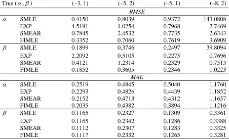
population distribution of X. These are the full information MLEs ˆα_fimle and ˆβ_fimle (FIMLE) that

assume knowledge of the non-sample values of X, the smearing estimators αˆ_smear and βˆ_smear (SMEAR) that only require the non-sample mean of X and the expansion estimators ˆα_exp and

ˆ

β_exp (EXP) that do not require any information about the non-sample distribution of X. The

sample-based MLEs were computed using the glm function in R, with its default options, while the MLEs utilising auxiliary information were calculated using the nlm function in R, with starting values α =log(yU)−log(1−yU) and β =0 . In each of 1000 independent simulations, a population of N independent and identically distributed values for X was generated from the standard lognormal distribution and corresponding values for Y generated under the linear logistic model. A sample of size n was then taken from this population using SRSWOR.

We see that there can be substantial gains when auxiliary population information is included in the modelling process, particularly when the probability that Y = 1 is small. We also note in passing that these gains become even more substantial as the sample size n decreases, however then greater care has to be taken with solution of the ML estimating equations. Observe that the expansion MLE sometimes provides the best RMSE performance, although this is not the case when one looks at MAE. However, the expansion MLE is conditionally biased, as is evident when one looks at the plots in Figure 2. This also shows that the sample-based MLE has a strong conditional bias, while both the smearing and full information MLEs are much better behaved.

4. MLE for a linear logistic model under case-control sampling

the sample data are obtained via some form of case-control sampling. In such cases the assumptions underpinning the saddlepoint and smearing approximations used in the development in the previous section are no longer valid. However, the basic strategy of using the approach of BCDTW to incorporate auxiliary population information into inference can still be used, provided the fact that the sample data are obtained via an informative sampling method (case-control sampling) is allowed for when taking conditional expectations. More specifically, we adopt the setup described in Scott and Wild (1997), and assume the existence of two sampling frames, one for the N₁ population units with values Y = 1 and one for the N₀ units with Y = 0. Independent simple random samples of size n₁ and n₀ respectively are then taken from these frames. Values of X are observed on the sample, and the aim again is to fit a linear logistic model to these data. By definition, we know N1 and hence try =N1−n1.

expectations no longer follow the same logistic model as in the population, so the approximations to the ML score function derived in the previous section need modification.

To start, consider the first situation described above, where individual X values for non-sample population units are known, but the corresponding values of Y are not. We continue to use the notation introduced in the previous section. From (14), we see that the key unknown quantity in the score function is E_s x_iy_i

r

∑

(

)

, where now, because of the case-control sampling, the y_i

values in the summation no longer follow the assumed population level logistic model. Following Scott and Wild (1997), we use Bayes Theorem to approximate the distribution of these values as N – n independent Bernoulli realisations with

πr(xi)=Pr

(

yi =1 |i∈r,xi

)

=

N1

−1

(N1−n1)π(xi) N1

−1

(N1−n1)π(xi)+N0

−1

(N0 −n0) 1

(

−π(xi)

)

.

With this set up, we can use the same saddlepoint arguments as in the previous section to approximate E_s

(

∑

_rxiyi

)

, replacing π(xi) in that development by πr(xi) above. This leads to a ‘full information’ score function with component (15a) as before, but with (15c) replaced by

sc2s(θ)=

∑

_sxi

(

yi −π(xi)

)

+ xiπr(xi) 1⎡⎣ +

(

1−πr(xi)

)

(br(try)−1)⎤⎦

−1

r

∑

−

∑

_rxiπ(xi) (18)

where b_r(t_ry)=exp π_r(x_i) 1

(

−π_r(x_i)

)

r

∑

⎡⎣ ⎤⎦−1

πr(xi) r

∑

−t_yr

⎡⎣ ⎤⎦

(

)

.

f(x_i,θ) r

∑

≈M₁n₁−1 f

(

Δ₁+x_i,θ

)

s1

∑

+M₀n₀−1 f

(

Δ₀ +x_i,θ

)

s0

∑

.

Here sd denotes the sample units with Y = d and Δ_d denotes our best estimate of the difference between the non-sample and sample means of X for those units with Y = d. Since we know the overall non-sample mean xr of X, we calculate Δd using a regression type estimate, i.e.

Δ_d =λ_dn_d−1s_xd2

(

λ₁2n₁−1s_x2₁+λ₀2n₀−1s_x2₀

)

−1

(

x_r −λ₁x_s1−λ₀x_s0

)

where λd =

(

Nd −nd

)

/ (N−n) and xsd, sxd

2

denote the mean and variance of X for the sample units with Y = d. The case-control version of the smearing approximation (17a) is then

sc_1smear(θ)= y_i U

∑

− π(x_i) s

∑

− Nd −nd

n_d

∑

sdπ(Δd +xi) d=0

1

∑

(19a)

while the corresponding case-control version of (17b) is

sc2smear(θ)=

∑

_sxi

(

yi −π(xi)

)

−

Nd −nd n_d ⎛ ⎝⎜

⎞

⎠⎟

∑

_sd

(

Δd+xi

)

π(Δd +xi) d=0

1

∑

+ Nd −nd n_d ⎛ ⎝⎜

⎞

⎠⎟

(

Δd +xi

)

πr(Δd +xi) 1+

{

1−πr(Δd +xi)

}

bsmear cc

(t_ry)−1

{

}

⎡⎣ ⎤⎦−1

s

∑

d=0 1

∑

(19b)

where

b_smearcc (t_ry)=exp Nd −nd nd d=0

1

∑

π_r(Δ_d +x_i) 1

(

−π_r(Δ_d +x_i)

)

sd

∑

⎡ ⎣ ⎢ ⎤ ⎦ ⎥ −1

N_d −n_d nd

π_r(Δ_d +x_i) sd

∑

d=0 1

∑

−t_yr

⎡ ⎣ ⎢ ⎤ ⎦ ⎥ ⎛ ⎝ ⎜ ⎞ ⎠ ⎟.

When x_r is also unknown, we replace x_rd by x_sd above. This is equivalent to setting Δd =0 in (19) and corresponds to using stratified expansion estimators for the expected values of the unknown non-sample components of the score function.

and are denoted by SMEAR. Finally, those obtained by solving (19) with Δ_d =0 are referred to as expansion MLEs and are denoted by EXP.

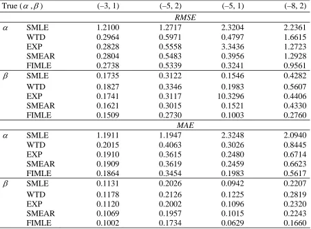
Table 4 sets out simulation results for the above approximate MLEs as well as for the standard sample-based MLEs αˆ_smle and βˆ_smle (SMLE). Prentice and Pyke (1979) showed that

ˆ

β_smle provides a good approximation to the actual MLE of this parameter under case-control sampling. In addition we show results for the maximum pseudo-likelihood estimates, defined by solving weighted versions of the sample-based MLE estimating equations, with weights given by w_i =N₀n₀−1I(y_i =0)+N₁n₁−1I(y_i =1) , and are denoted by WTD. We also computed the maximum ‘pseudo-model’ likelihood estimates proposed by Scott and Wild (1997) for case-control sampling, but do not show results for them since these were almost identical to those for SMLE for β and tended to be unstable for α .

The simulation methodology used to obtain the results in Table 4 is identical to that used in Table 3, with the exception that sampling here is carried out using the stratified case-control design described at the start of this section. Note that SMLE and WTD estimates were computed using the glm function in R (without and with weights respectively) and with default settings. The FIMLE, SMEAR and EXP approximations to the MLEs that utilised auxiliary information were all computed by using the nlm function in R to solve the relevant estimating equations.

4. Discussion

The two most important conclusions that we draw from the results set out in this paper is that it pays to include population level auxiliary information when modelling sample survey data, and that the BCDTW likelihood framework offers a viable approach to achieving this aim. Obviously, the more auxiliary information one has available, the more significant the improvement in one’s inference. However, even marginal information (e.g. knowledge of population means for the model variables) can be extremely useful when integrated with the sample data within this framework. In general, use of the BCDTW framework requires the evaluation of conditional expectations that depend both on the assumed population model as well as on the method used to select the sample. For the important case of a logistic population model, the saddlepoint and smearing approximations to these conditional expectations that we describe in this paper seem to work well and should be useful in extending our results in practice.

This paper does not include results on interval estimation when auxiliary population data are integrated into likelihood inference. The BCDTW framework also covers this situation, and in the Appendix we show how the information function can be extended to allow for the auxiliary information in the case of a logistic model, including appropriate saddlepoint approximations. An important use of this function is in evaluating the extra information for parametric inference provided by the auxiliary information, e.g. along the lines set out in Steel et. al. (2004).

References

Breckling, J.U., Chambers, R.L., Dorfman, A.H., Tam, S.M. and Welsh, A.H. (1994). Maximum likelihood inference from survey data. International Statistical Review, 62, 349 - 363. Chambers, R.L. (1996). Robust case-weighting for multipurpose establishment surveys. Journal

of Official Statistics, 12, 3 - 32.

Chambers, R.L., Dorfman, A.H. and Wang, S. (1998). Limited information likelihood analysis of survey data. Journal of the Royal Statistical Society, Series B, 60, 397 - 412.

Deville, J.C. and Särndal, C.E. (1992). Calibration estimators in survey sampling. Journal of the American Statistical Association, 87, 376 - 382.

Duan, N. (1983). Smearing estimate: A nonparametric retransformation estimate. Journal of the American Statistical Association, 78, 605 - 610.

Handcock, M., Rendall, M. and Cheadle, J. (2005). Improved regression estimation of a multivariate relationship with population data on the bivariate relationship. Sociological Methodology, 35, 291 - 334.

Imbens, G.W. and Lancaster, T. (1994). Combining micro and macro data in microeconometric models. Review of Economic Studies, 61, 655 - 680.

Prentice, R.L. and Pyke, R. (1979). Logistic disease incidence models and case-control studies. Biometrika, 66, 403 - 411.

Qin, J. (2000). Combining parametric and empirical likelihoods. Biometrika, 87, 484 - 490. Scott, A.J. and Wild, C.J. (1997). Fitting regression models to case-control data by maximum

likelihood. Biometrika, 84, 57 - 71.

Appendix

A. Saddlepoint Approximations

We first consider approximation of R1i. Let yv be the mean of Y over the set v, with Nv the corresponding number of observations. Further, let gv(d)=Pr(yv=d|xv) and πi =π(xi) . Then, fort_ry >0

R1i =

g_r(i)

{

(t_ry −1) /N_r(i)

}

πigr(i)

{

(try−1) /Nr(i)

}

+(1−πi)gr(i)(try /Nr(i))

= 1+(1−πi)

g_r(i)(t_ry /N_r(i))

g_r(i)

{

(t_ry −1) /N_r(i)

}

−1

⎡

⎣ ⎢ ⎢

⎤

⎦ ⎥ ⎥ ⎛

⎝

⎜⎜ ⎞_⎠⎟⎟

−1

. (A.1)

It follows that the major problem is to approximate ⎡⎣g_r(i)

{

(t_ry−1) /N_r(i)

}

⎤⎦−1g_r(i)(t_ry /N_r(i))

accurately. Now the cumulant generating function of

∑

_νyj is Kv(u)= log{πje u +

(1−πj)}

ν

∑

.

For any d∈(0,1) the saddlepoint approximation to g_v(d) is then

hv(d)=

Nv {2πK′′v(ud)}

1/ 2exp{Kv(ud)−Nvudd}

where ud is called the saddlepoint, and is defined as the solution of ′

Kv(u) /Nv=d. (A.2)

Standard arguments can be used to show that h_v(d)=g_v(d){1+O(1

N_v)} under general regularity conditions. That is, the saddlepoint approximation has relative error of order N_v−1. Substituting

d=d₁ =t_ry/N_r(i) or d=d₂ =(t_ry −1) /N_r(i) in h_r(i)(d) , we then have

g_r(i)(t_ry /N_r(i))

gr(i)

{

(try −1) /Nr(i)

}

= hr(i)(try /Nr(i))

hr(i)

{

(try−1) /Nr(i)

}

{1+O(1

N)}=exp{−ud₁}{1+O(

1

N)} (A.3) where the last equation is due to the identity

K_r(i)(u_d

1)−Nr(i)ud1d1−

{

Kr(i)(ud2)−Nr(i)ud2d2

}

=Nr(i)ud1(d2 −d1)+O(

1

N)= −ud1 +O(

1

From the central limit theorem N_ν−1/ 2 (y_j −π_j) v

∑

→N(0,γ2) as N_v→ ∞, where

γ2 =

limN_ν−1

∑

_vπj(1−πj). It follows that we can focus on the normal deviation values of

t_ry: t_ry− π_j =O

( )

N r(i)

∑

. For such values of t_ry, u_d

1 =O N

−1/ 2

( )

. In fact, from (A.2), it can be

seen that

u_d 1 =

t_ry− Σ_r(i)π_j Σr(i)πj(1−πj)

+O 1 N ⎛ ⎝⎜ ⎞⎠⎟ =

t_ry− Σ_rπ_j Σrπj(1−πj)

+O 1 N ⎛

⎝⎜ ⎞⎠⎟. (A.4)

By (A.1), (A.3) and (A.4), an approximation to R_1i is then

R_1i =⎡⎣1+(1−π_i)

{

b(t_ry)−1

}

⎤⎦−1 1+O 1 N ⎛ ⎝⎜ ⎞⎠⎟ ⎧ ⎨ ⎩ ⎫ ⎬

⎭ (A.5)

with b(try)=exp ⎡⎣

∑

_rπj(1−πj)⎤⎦

−1

πj r

∑

−try

⎡⎣ ⎤⎦

{

}

. It immediately follows that (15b) can be

approximated by

sc_s(β)≈ x_i(y_i −π_i) s

∑

− x_iπ_i

(

1−[1+(1−π_i){b(t_ry)−1}]−1

)

r

∑

. (A.6)

When non-sample values of X are unavailable, but their mean xr is known, we can combine the saddlepoint approximation developed above with a smearing approximation to again approximate the logistic score function. In particular, this procedure can be used together with (A.6) to approximate the second part of (16b). We continue to use (17a) to approximate (16a). By (A.6),

sc_s(β)≈ x_i(y_i−π_i)

s

∑

−

{

x_r +(x_i−x_r)

}

π_i

(

1−⎡⎣1+(1−π_i)

{

b(t_ry)−1

}

⎤⎦−1

)

r

∑

≈ x_i(y_i−π_i)

s

∑

− N−n

n

⎛

⎝⎜ ⎞⎠⎟

(

xr −xs+xi

)

πi,adj 1−⎡⎣1+(1−πi,adj)

{

b(try)−1

}

⎤⎦

−1

(

)

s

∑

≈ x_i(y_i−π_i)

s

∑

− N−n

n

⎛

⎝⎜ ⎞⎠⎟

(

xr −xs+xi

)

πi,adj 1−⎡⎣1+(1−πi,adj)

{

badj(try)−1

}

⎤⎦

π_i,adj =exp

{

β(x_r−x_s)+α+βx_i

}

/ 1⎡⎣ +exp

{

β(x_r−x_s)+α+βx_i

}

⎤⎦

and

b_adj(t_ry)=exp π_i,adj

(

1−π_i,adj

)

s

∑

⎡⎣ ⎤⎦−1

π_i,adj s

∑

− n

N−ntry ⎡ ⎣⎢ ⎤ ⎦⎥ ⎧ ⎨ ⎩ ⎫ ⎬ ⎭.

Note that the last two approximation steps in (A.7) used smearing approximations repeatedly. B. The Information Function in the Logistic Case

Within the BCDTW framework the information function for parametric likelihood inference is the conditional expectation of the population level information function minus the conditional variance of the population level score function. As always, conditioning here is with respect to the observed survey data as well as the auxiliary information. In the logistic case the information function components are therefore given by

info_s(α,α)=E_s

(

info(α,α)

)

−Var_s

(

sc(α)

)

=E_s π(x_i)(1−π(x_i))

U

∑

−Var_s (y_i −π(x_i))

U

∑

(

)

= π(x_i)(1−π(x_i))

U

∑

info_s(α,β)=E_s

(

info(α,β)

)

−Cov_s

(

sc(α),sc(β)

)

=E_s x_iπ(x_i)(1−π(x_i))

U

∑

−Cov_s (y_i−π(x_i))

U

∑

, x_i(y_i −π(x_i))

U

∑

(

)

= x_iπ(x_i)(1−π(x_i))

U

∑

info_s(β,β)=E_s

(

info(β,β)

)

−Var_s

(

sc(β)

)

= x_i2π(x_i)(1−π(x_i))

U

∑

−Var_s

(

∑

_Uxi(yi−π(xi))

)

= x_i2π

(x_i)(1−π(x_i)) U

∑

−Var_s x_iy_i U

∑

(

)

where

Var_s y_ix_i U

∑

(

)

=Var y_ix_i r

∑

| y_i r

∑

=t_ry,x_r

(

)

=E y_iy_jx_ix_j j∈r

∑

i∈r

∑

| y_i

r

∑

=t_ry,x_r

(

)

− E y_ix_i

r

∑

| y_i r

∑

=t_ry,x_r

(

)

⎡

⎣ ⎤⎦

2

E y_iy_jx_ix_j j∈r

∑

i∈r

∑

| y_i

r

∑

=t_ry,x_r

(

)

= xi

2

E y

(

i |

∑

_ryk =try,xr

)

r

∑

+

∑

_i∈r

∑

_j≠i∈rx_ix_jE y

(

iyj |

∑

_ryj =try,xr

)

= x_i2π(x_i)R_1i

r

∑

+ x_ix_jπ(x_i)π(x_j)R_2ij j≠i∈r

∑

i∈r

∑

E y_ix_i

r

∑

| y_i

r

∑

=t_ry,x_r

(

)

⎡

⎣ ⎤⎦

2

=

∑

_rxiπ(xi)Pr

(

∑

_r(i)yj =try −1 |xr(i)

)

Pr y_k

r

∑

=t_ry |x_r

(

)

⎡ ⎣ ⎢ ⎢ ⎤ ⎦ ⎥ ⎥ 2

= xi

2π2 (xi)R1i

2

r

∑

+

∑

_i∈r

∑

_j≠i∈rxixjπ(xi)π(xj)R1iR1j

and R_2ij = Pr y_k r

∑

=t_ry |x_r

(

)

⎡

⎣ ⎤⎦

−1

Pr y_k

r(ij)

∑

=t_ry−2 |x_r(ij)

(

)

. It follows

Var_s y_ix_i U

∑

(

)

= x_i2π

(x_i)R_1i

(

1−π(x_i)R_1i

)

r

∑

+ x_ix_jπ(x_i)π(x_j)(R_2ij −R_1iR_1j) j≠i∈r

∑

i∈r

∑

.

A saddlepoint approximation to R2ij similar to that developed above for R1i can be written down. This is based on the fact that the denominator of R_2ij can be expressed as

Pr y_k =t_ry|x_r

r

∑

(

)

=π_iπ_jPr y_k =t_ry −2 |x_r(ij)

r(ij)

∑

(

)

+

{

πi(1−πj)+(1−πi)πj

}

Pr

(

∑

_r(ij)yk =try−1 |xr(ij)

)

+(1−π_i)(1−π_j)Pr y_k =t_ry |x_r(ij)

r(ij)

∑

(

)

leading to

R_2ij = π_iπ_j +(π_i+π_j−2π_iπ_j)Pr

(

Σr(ij)yk =try −1 |xr(ij)

)

Pr

(

Σ_r(ij)y_k =t_ry −2 |x_r(ij)

)

⎧ ⎨ ⎪ ⎩⎪

+(1−π_i)(1−π_j) Pr

(

Σr(ij)yk =try |xr(ij)

)

Pr

(

Σ_r(ij)y_k =t_ry −2 |x_r(ij)

)

⎫ ⎬ ⎪ ⎭⎪ −1 .

Using the same saddlepoint approximation technique as that used forR_1i, the two ratios in this expression can be approximated by b(t_ry −1) and b2(t_ry−1) respectively. That is,

R_2ij =

{

π_iπ_j +(π_i +π_j−2π_iπ_j)b(t_ry−1)+(1−π_i)(1−π_j)b2(t_ry−1)

}

1+O 1

N

( )

[image:28.612.68.546.156.417.2]

Table 1 Root mean squared errors (RMSE) and median absolute errors (MAE) under SRSWOR and a linear population model with α = 5, β = 1 and σ2 = 1. Values of X drawn from the standard lognormal distribution.

RMSE MAE

N = 500 n = 20

N = 1000 n = 50

N = 5000 n = 200

N = 500 n = 20

N = 1000 n = 50

N = 5000 n = 200

α SMLE 0.3217 0.1929 0.0922 0.2132 0.1339 0.0594

LIMCAL 0.5935 0.2100 0.0977 0.2274 0.1276 0.0601

LIMMLE 3.3769 0.3668 0.0676 0.1948 0.1015 0.0429

CALW 1.3925 0.1658 0.0654 0.1803 0.0947 0.0421

FIMLE 0.2554 0.1408 0.0631 0.1582 0.0869 0.0399

β SMLE 0.1679 0.0867 0.0374 0.0935 0.0517 0.0234

LIMCAL 0.4109 0.0977 0.0429 0.1018 0.0557 0.0246

LIMMLE 3.2881 0.3327 0.0494 0.1270 0.0655 0.0310

CALW 0.8008 0.0994 0.0391 0.1069 0.0553 0.0254

FIMLE 0.1550 0.0843 0.0375 0.0884 0.0522 0.0234

σ2

SMLE 0.3154 0.1975 0.1022 0.2350 0.1361 0.0741

LIMCAL 0.4186 0.2033 0.1024 0.2557 0.1398 0.0743

LIMMLE 107.4689 0.8051 0.1019 0.2440 0.1341 0.0738

CALW 0.4258 0.2152 0.1036 0.2692 0.1509 0.0735

[image:29.612.67.549.161.661.2]

Table 2 Root mean squared errors (RMSE) and median absolute errors (MAE) under PPX and PPY sampling and a linear population model with α = 5, β = 1 and σ2 = 1. Values of X drawn from the standard lognormal distribution.

RMSE MAE

N = 500 n = 20

N = 1000 n = 50

N = 5000 n = 200

N = 500 n = 20

N = 1000 n = 50

N = 5000 n = 200

PPX Sampling

α SMLE 0.3285 0.1993 0.0927 0.2065 0.1312 0.0629

LIMCAL 1.3901 3.3726 0.1824 0.3057 0.1939 0.1320

LIMMLE 0.2359 0.1715 0.1170 0.1665 0.1224 0.0943

CALW 5.0604 2.5311 0.0466 0.1552 0.0763 0.0270

FIMLE 0.1116 0.0611 0.0263 0.0651 0.0410 0.0169

β SMLE 0.0715 0.0369 0.0157 0.0368 0.0224 0.0102

LIMCAL 0.7589 1.8295 0.0413 0.0934 0.0500 0.0187

LIMMLE 0.0817 0.0414 0.0170 0.0386 0.0231 0.0109

CALW 2.9475 1.6181 0.0272 0.0901 0.0411 0.0152

FIMLE 0.0612 0.0316 0.0139 0.0319 0.0197 0.0091

σ2

SMLE 0.3272 0.1984 0.1020 0.2429 0.1362 0.0675

LIMCAL 0.6624 0.9780 0.1137 0.2723 0.1567 0.0786

LIMMLE 0.3416 0.2110 0.1076 0.2280 0.1356 0.0698

CALW 1.8410 0.5481 0.1155 0.2877 0.1579 0.0782

FIMLE 0.3174 0.1954 0.1020 0.2347 0.1362 0.0677

PPY Sampling

α SMLE 0.3558 0.2483 0.1906 0.2310 0.1825 0.1726

LIMCAL 5.3714 1.6835 3.9844 0.2343 0.1723 0.1474

LIMMLE 0.6531 0.1500 0.0939 0.1589 0.0945 0.0689

CALW 2.2143 4.8633 16.6698 0.1626 0.1059 0.0873

FIMLE 0.1953 0.0958 0.0408 0.0974 0.0558 0.0255

β SMLE 0.1253 0.0580 0.0251 0.0619 0.0337 0.0158

LIMCAL 3.8975 1.1988 2.4283 0.0957 0.0633 0.0519

LIMMLE 0.5743 0.0880 0.0310 0.0671 0.0376 0.0183

CALW 1.2909 2.9607 10.1346 0.0981 0.0644 0.0527

FIMLE 0.1178 0.0555 0.0232 0.0603 0.0311 0.0136

σ2

SMLE 0.3160 0.2035 0.0998 0.2343 0.1462 0.0682

LIMCAL 0.9376 0.3779 0.5802 0.2552 0.1563 0.0759

LIMMLE 2.1472 0.2027 0.0974 0.2252 0.1473 0.0672

CALW 0.9910 1.1900 2.7521 0.2926 0.1802 0.0914

[image:30.612.81.533.155.430.2]

Table 3 Root mean squared errors (RMSE) and median absolute errors (MAE) for the linear logistic model under SRSWOR and given different amounts of auxiliary information on X. In all cases N = 5000 and n = 200.Values of X drawn from the standard lognormal distribution.

True (α,β) (–3, 1) (–5, 2) (–5, 1) (–8, 2)

RMSE

α SMLE 0.4150 0.8039 0.9372 143.0808

EXP 4.5191 1.0254 0.7968 2.7469

SMEAR 0.7845 2.4532 0.7735 2.6343

FIMLE 0.3352 0.7060 0.7619 3.6909

β SMLE 0.1899 0.3746 0.2497 39.8094

EXP 2.2092 0.5105 0.2275 0.7696

SMEAR 0.4121 1.2314 0.2329 0.7513

FIMLE 0.1852 0.3605 0.2346 1.0223

MAE

α SMLE 0.2519 0.4845 0.5040 1.1760

EXP 0.2293 0.4826 0.4439 1.1852

SMEAR 0.2152 0.4713 0.4312 1.1657

FIMLE 0.2035 0.4382 0.3894 1.1216

β SMLE 0.1165 0.2327 0.1309 0.3361

EXP 0.1165 0.2342 0.1286 0.3388

SMEAR 0.1112 0.2307 0.1283 0.3325

[image:31.612.82.534.183.516.2]

Table 4 Root mean squared errors (RMSE) and median absolute errors (MAE) for the linear logistic model under case-control sampling and given different amounts of auxiliary information on X. In all cases N = 5000 and n1=n0 =100 . Values of X drawn from the standard lognormal

distribution.

True (α,β) (–3, 1) (–5, 2) (–5, 1) (–8, 2)

RMSE

α SMLE 1.2100 1.2717 2.3204 2.2361

WTD 0.2964 0.5971 0.4797 1.6615

EXP 0.2828 0.5558 3.3436 1.2723

SMEAR 0.2804 0.5483 0.3956 1.2928

FIMLE 0.2738 0.5339 0.3241 0.9561

β SMLE 0.1735 0.3122 0.1546 0.4282

WTD 0.1827 0.3346 0.1983 0.5607

EXP 0.1741 0.3117 10.3296 0.4406

SMEAR 0.1621 0.3015 0.1521 0.4330

FIMLE 0.1509 0.2730 0.1003 0.2760

MAE

α SMLE 1.1911 1.1947 2.3248 2.0940

WTD 0.2015 0.4063 0.3026 0.8445

EXP 0.1910 0.3615 0.2480 0.6714

SMEAR 0.1909 0.3619 0.2459 0.6623

FIMLE 0.1864 0.3454 0.1983 0.5617

β SMLE 0.1131 0.2026 0.0942 0.2207

WTD 0.1178 0.2126 0.1225 0.2819

EXP 0.1120 0.2002 0.1096 0.2320

SMEAR 0.1069 0.1957 0.1015 0.2243

Figure 1 Simulated estimation errors for α in the linear model (1). The true value of α is 5 and sampling is SRSWOR with N = 1000 and n = 50. Errors are ordered along the horizontal axis by the rank of the sample Y-mean ys. Solid red line shows median estimation error by decile group of these sample means. Errors greater than 0.5 in absolute value are not shown. Out of a total of 1000 simulated errors, there were 9 such values for SMLE, 22 for LIMCAL, 30 for LIMMLE, 9 for CALW and 4 each for PRED and FIMLE.

QuickTime™ and a TIFF (Uncompressed) decompressor

are needed to see this picture.

QuickTime™ and a TIFF (Uncompressed) decompressor

are needed to see this picture.

QuickTime™ and a TIFF (Uncompressed) decompressor

are needed to see this picture.

QuickTime™ and a TIFF (Uncompressed) decompressor

are needed to see this picture.

QuickTime™ and a TIFF (Uncompressed) decompressor