Dam Management With Imperfect Models:
Bayesian Model Averaging and Neural Network
Control
Paul J. Darwen
School of Business, James Cook University, Brisbane Campus 349 Queen Street, Brisbane, Queensland, Australia
Abstract. Dam management is a controversial control problem for two reasons. Firstly, models are (by definition) crudely simplified versions of reality. Secondly, historical rainfall data is limited and noisy. As a re-sult, there is no agreement on the “best” control policy for running a dam. Bayesian model averaging is theoretically a good way to cope with these difficulties, but in practice it degrades under two approximations: discretizing the parameter space, and excluding models with a low prob-ability of being correct. This paper explores the practical aspects of how Bayesian model averaging with a neural network controller can improve dam management and flood control.
1
Motivation
A dam on a river has two functions, to store water for dry times, and to prevent flooding. Unfortunately, these two functions are diametrically opposed:
– To prevent flooding, you should gradually let out all the water from the dam, so that it can catch a future flood.
– To store water for dry times, you should never let out any water.
The dam control problem is stark: how much water should we keep in the dam, and how much should we let out? Currently there is no consensus answer. Section 3.1 looks at the simple control policy of always letting the water level down to some fixed percentage of the dam’s capacity. Section 3.3 considers a more elaborate control policy using a neural network found by expectation maximization, either:
– By finding the single model that best fits historical data (using expectation maximization again), or;
– By finding a whole distribution of plausible models with Bayesian model averaging [1], an approach which is theoretically better [4, page 175].
2
A Dam Control Problem
Imagine a river with a dam that has controllable release gates, so the dam’s water level can be reduced to any desired level. To calibrate a rainfall model, only 100 years of historical rainfall data exist. For a future 50-year period, the two conflicting aims are to avoid either of these disasters:
– Avoid flooding, when the dam level reaches rises above 100%.
– Avoid running empty, when the dam level reaches 0%.
Evidence suggests that the weather in eastern Australia follows a 5-year cycle of wet and dry, with both shorter- and longer-term cycles to complicate matters [3]. To capture that, this paper makes up a stochastic rainfall function that gives river flow at time t (in months) by taking random samples from a lognormal function with standard deviationσ= 0.1 and meanµgiven by:
µ= ln(2 + (0.3299928×tanh(3.3×sin(t/9.55)) (1)
+0.3345885×tanh(3.4×sin(t/7.00))
+0.3354186×tanh(3.5×sin(t/4.15))))
Equation 1 has three flood/drought cycles with roughly equal importance, with periods of 4.15, 7, and 9.55 months. The rest is merely to make it more complicated than the simple model described next in Section 2.1.
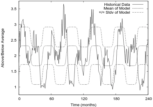
To generate 100 years of historical data, running this rainfall function with a particular random number seed gives the historical data shown in Figure 1.
1 1.5 2 2.5 3 3.5
0 60 120 180 240
Above/Below Average
Time (months)
[image:2.595.176.439.423.607.2]Historical Data Mean of Model +/= Stdv of Model
2.1 A Crude Model
All rainfall models are simpler than the real world, and here the model in Equa-tion 2 is too simple to capture the actual rainfall funcEqua-tion in EquaEqua-tion 1. Here, a simple stochastic model has the following form, with mean river flowµset to:
µ= 2.0 +w0∗tanh(4.0∗sin(t/w1)) (2)
That is, the model assumes a cycle from flood to drought, where the two model parameters arew0 the amplitude andw1 the duration of that cycle, and it predicts the river’s mean flow at time tin months. An example of this model for a particular choice of parametersw0 andw1 is in Figure 1.
To give the model a stochastic flavour, the prediction is a random sampling from a normal distribution with mean given by Equation 2 and standard devia-tionσ= 0.6. Any negative predictions are set to zero.
2.2 A Control Function
A popular control policy is to set a single parameter, namely how much of the dam’s capacity to fill with water, with the unused capacity being a “flood compartment”. This policy will be evaluated later in Section 3.1.
A more elaborate controller could be a neural network, and this paper uses the simplest kind: a sigmoid function equivalent to a one-node neural network.
θ(u0, u1, x, t) = 1
1 +eu0+u1x (3)
The sigmoid functionθin Equation 3 has bias u0 and weightu1, and takes inputx(w0, w1, t) the water level of the dam at time tas predicted by a model with parameters w0 and w1 from Equation 2. The sigmoid function θ is the desired water level that the dam should be lowered to. Of course, if the dam’s water level is already less than that, then no water need be released.
As a sigmoid function can take an S-shape, the general aim of this controller function is to suggest a lower dam level if wet weather is predicted, and to suggest a higher dam level if dry weather is predicted.
2.3 The Single Best-Fit Model versus Bayesian Model Averaging
A popular approach for finding a controller is to calibrate the model’s parameters to the historical data, and then calibrate a controller to that single best-fit model. To find that single best-fit model, expectation maximization is a popular approach: it finds the model that has the highest probability of being correct, given the data [2]. For the historical data in Figure 1, the most probable model hasw0 = 0.32 andw1 = 6.9964 in Equation 2. Figure 1 shows this model.
0.2
0.25
0.3
0.35
0.4 4 5 6
7 8 9 10 0
0.002 0.004 0.006 0.008
Posterior probability
w0
w1
Posterior probability
[image:4.595.141.471.119.268.2]0 0.002 0.004 0.006 0.008
Fig. 2. The probability distribution of plausible models. The single most-probable model is the one at the peak of the highest hill.
In the Bayesian model averaging approach, the aim is to iterate over all those plausible models to find the probability that a model is correct, given the historical data. Figure 2 shows this probability distribution for our test problem. The highest point in that distribution represents the most probable model, at parameters w0 = 0.32 and w1 = 6.9964. But picking the highest point in the probability distribution (i.e., the best-fit model) ignores all those other less-probable models that are still plausible, throwing away much of the information in the historical data.
In this paper, the problem is not to find the single “best” model, but instead to come up with an adequate controller despite having a too-simple model.
2.4 Two Approximations to Bayesian Model Averaging
Bayesian model averaging is theoretically the better method [4, page 175], but that proof assumes a continuous world. In the messy world of numerical approx-imations, there are trade-offs. This section describes two approximations.
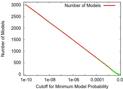
0 500 1000 1500 2000 2500 3000
1e-10 1e-08 1e-06 0.0001 0.01
Number of Models
[image:5.595.205.405.121.266.2]Cutoff for Minimum Model Probability Number of Models
Fig. 3.There are an unlimited number of low-probability models, so this paper uses a cutoff of 10−6, which makes for 1,489 models.
3
Results
3.1 A Fixed Level Is Not A Good Policy
A simple control policy is to gradually release water from the dam until the level is down to some fixed percentage of capacity, so the unused dam space can be a “flood compartment”. This section evaluates that kind of policy.
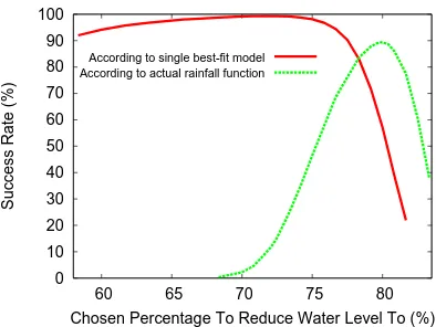
Take the single model that best fits the historical data, and use it to evaluate various fixed levels by doing Monte Carlo simulation of many possible 50-year futures. The peak of the solid line in Figure 4 shows that the single best-fit model predicts a fixed level of 71.65% would be the best water level to keep the dam at, and doing so should prevent disaster (either the dam over-filling, or running empty) with a probability of 99.35% over the next 50 years. Sounds pretty good, if you trust that single best-fit model!
Unfortunately, the dashed line in Figure 4 uses the true, unseen function that generates rainfall (from Equation 1) to evaluate the true probability of success. If you run the dam at a constant water level of 71.65% as suggested by the single best-fit model, then your true probability of success is a lousy 9.4%, much less than the 99.35% that the single best-fit model has led you to believe.
3.2 A Neural Network Controller from the Single Best-Fit Model
Take the single best model, which is the peak of Figure 2), and use it to find the best controller function. That single best model says its best controller should have a success rate of about 98%, which sounds pretty safe.
0 10 20 30 40 50 60 70 80 90 100
60 65 70 75 80
Success Rate (%)
Chosen Percentage To Reduce Water Level To (%) According to single best-fit model
[image:6.595.206.403.118.266.2]According to actual rainfall function
Fig. 4.A simple control policy is to gradually release water to bring the level down to some fixed percentage. Using the single model that best fits the historical data, this shows how well the fixed-level approach works according to that single best model, and according to the actual, unseen rainfall function. Keeping the water level at 71.65% (as the best-fit model suggests) would give a real success rate of only 9.4%.
3.3 A Neural Network Controller from Bayesian Model Averaging
Bayesian model averaging generates the whole distribution of models shown in Figure 2. This paper discretizes that distribution and then ignores the low-probability models, as described in Section 2.4.
So here, the best controller is the one that performs best, according to the weighted vote of all 1,489 models. The weighting is according to each model’s probability of being correct. This approach takes about 1,498 times as much computer time as using the single best-fit model. The best controller should get a success rate of 98%, according to those models, showing that the controller function is not the bottleneck — whatever the model(s), there is a controller which supposedly will have a 98% success rate, according to those models.
Taking that winning controller from Bayesian model averaging, and running it through 400,000 simulated 50-year futures using the true rainfall function gives a true success rate of 45.796%. That’s better than the 32.319% from the single best-fit model in Section 3.2, and much better than the lousy 9.4% from using a fixed level back in Section 3.1. These differences are statistically significant.
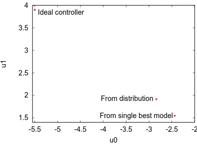
The single best-fit model gives a controller at the parametersu0 =−2.4375 andu1= 1.546875. In contrast, the controller from Bayesian model averaging is atu0=−2.83984375 andu1= +1.9140625, a substantial difference.
1.5 2 2.5 3 3.5 4
-5.5 -5 -4.5 -4 -3.5 -3 -2.5 -2
u1
u0 Ideal controller
From distribution
[image:7.595.206.407.119.267.2]From single best model
Fig. 5. The two controller functions, one found from the single best model, and the other from a Bayesian distribution of all plausible models, are shown here with the ideal controller, found by using the (usually unseen) function that generates rainfall. The Bayesian approach is closer to the ideal.
4
Discussion and Conclusion
Models are merely simplified, abstracted version of the real thing. A more re-alistic model would have more than the 2 parameters in Equation 2. However, models with a many free parameters require more data. Any practical rainfall model cannot have a large number of free parameters, due to the shortage of historical data. This avoids a combinatorial explosion from a high-dimensional space of model parameters. So long as the space of plausible models has rea-sonably low dimensions, then iterating through that space of models should be feasible for the Bayesian model averaging approach.
In this problem, the complexity of the neural network controller and the algorithm for optimizing that controller were not the bottlenecks that prevent success — in fact, even the simple controller used here was good enough for a 98% success rate. The bottleneck is that the model is too simple. For such models, Bayesian model averaging is a practical way do dam management and similar control problems.
References
1. Hoeting, J.A., Madigan, D., Raftery, A.E., Volinsky, C.T.: Bayesian model averag-ing: A tutorial. Statistical Science 14(4), 382–417 (1999)
2. Jeffreys, H.: Theory of Probability. The International Series of Monographs on Physics, Oxford University Press, 1 edn. (1939)
3. Mazzarella, A., Giuliacci, A., Liritzis, I.: On the 60-month cycle of multivariate ENSO index. Theoretical and Applied Climatology 100, 2327 (2010)