Model Selection for Semi-Supervised Clustering
Mojgan Pourrajabi
University of Alberta Edmonton, AB, CanadaDavoud Moulavi
University of Alberta Edmonton, AB, CanadaRicardo J. G. B. Campello
University of São PauloSão Carlos, Brazil
Arthur Zimek
Ludwig-Maximilians-Universität München Munich, Germany
Jörg Sander
University of Alberta Edmonton, AB, CanadaRandy Goebel
University of Alberta Edmonton, AB, Canada[email protected]
ABSTRACT
Although there is a large and growing literature that tackles the semi-supervised clustering problem (i.e., using some la-beled objects or cluster-guiding constraints like “must-link” or “cannot-link”), the evaluation of semi-supervised cluster-ing approaches has rarely been discussed. The application of cross-validation techniques, for example, is far from straight-forward in the semi-supervised setting, yet the problems as-sociated with evaluation have yet to be addressed. Here we summarize these problems and provide a solution.
Furthermore, in order to demonstrate practical applica-bility of semi-supervised clustering methods, we provide a method for model selection in semi-supervised clustering
based on this sound evaluation procedure. Our method
allows the user to select, based on the available informa-tion (labels or constraints), the most appropriate clustering model (e.g., number of clusters, density-parameters) for a given problem.
1.
INTRODUCTION
Cluster analysis is a fundamental conceptual problem in data mining, in which one aims to distinguish a finite set of categories to describe a data set, according to similari-ties or relationships among its objects [13, 20, 23]. It is an interdisciplinary field that includes elements of disciplines such as statistics, algorithms, machine learning, and pattern recognition. Clustering methods have broad applicability in many areas, including marketing and finance, bioinformat-ics, medicine and psychiatry, sociology, numerical taxonomy, archaeology, image segmentation, web mining, and anomaly detection, to mention just a few [2, 16, 21, 22].
The literature on data clustering is extensive (e.g., see [19] for a recent survey), and a variety of clustering al-gorithms have been developed over the past five decades [7, 21, 26, 34, 41]. Despite the rapid development of this area,
(c) 2014, Copyright is with the authors. Published in Proc. 17th Inter-national Conference on Extending Database Technology (EDBT), March 24-28, 2014, Athens, Greece: ISBN 978-3-89318065-3, on OpenProceed-ings.org. Distribution of this paper is permitted under the terms of the Cre-ative Commons license CC-by-nc-nd 4.0
an issue that remains critical and of primary importance is the evaluation of clustering results. In particular, it is well-known that different clustering algorithms — or even the same algorithm with different configurations for its
pa-rameters (e.g., the number of clusterskwhen this quantity
is required as an input) — may come up with significantly different solutions when applied to the same data. In this scenario, which solution is best? This question is essentially
the fundamental problem ofmodel selection, i.e., choosing a
particular algorithm and/or a particular parametrization of this algorithm amongst a diverse collection of alternatives.
A solution to the model selection problem is not trivial because, unlike pattern classification, cluster analysis is not
a supervised task. Even the concept ofcluster is quite
sub-jective, and may be defined in many different ways [13]. One possible approach for unsupervised model selection is to use (internal) relative clustering evaluation criteria as quantitative, commensurable measures of clustering qual-ity [20,30,36]. This approach, however, has two major short-comings [36]: (i) criteria that have become well-established in the literature are restricted to evaluating clusterings with volumetric (usually globular-shaped) clusters only; they are not appropriate for evaluating results involving arbitrarily-shaped (e.g. density-based) clusters; and (ii) it is well-known that the evaluations and performance of different existing criteria are highly data-dependent, in a way that makes it very difficult to choose one specific criterion for a particular data set.
Apart from unsupervised approaches, there has been a growing interest in semi-supervised clustering methods, which are methods developed to deal with partial information about object properties being clustered, usually given in the form of clustering constraints (e.g., instance-level pairwise con-straints) [12, 38], or in the form of a subset of pre-labeled data objects [9, 28]. The area of semi-supervised clustering has had more attention in recent years [6], with formulations of the problem being discussed from a theoretical perspec-tive [11] and algorithms being developed to deal with semi-supervision in a variety of ways, including metric learning [8] and (hard or soft) enforcement of constraint satisfaction [39]. In spite of these advances, the focus has been only on how to obtain (hopefully better) clustering solutions through semi-supervised guidance. The problem of model selection has been notably overlooked.
for finding Clustering Parameters”). The core idea of the framework is to select models that better fit the user-provided partial information, from the perspective of classification er-ror estimation based on a cross-validation procedure. Since a clustering algorithm provides a relative rather than abso-lute labeling of the data, our measure for the fit of avail-able semi-supervised information is designed so that we can properly estimate a classification error. We have developed and experimented with estimators conceived for two differ-ent scenarios: (i) when the user provides as an input to the framework a subset of labeled objects; or (ii) when the user provides a collection of instance-level pairwise constraints (should- and should-not-link constraints). The first scenario has broader applicability, because constraints can be ex-tracted from labels; so if labels are provided, the framework can be applied both to algorithms that work with labels, and to algorithms that work with constraints. However, in many applications only constraints may be available, so we also elaborate on this scenario.
The remainder of this paper is organized as follows. In
Section 2 we discuss the related work. In Section 3 we
present our framework for model selection in semi-supervised clustering. In Section 4 we report experiments involving real data sets. Finally, in Section 5 we address the conclusions.
2.
RELATED WORK
The evaluation of semi-supervised clustering results may involve two different problems. First, there is a problem of
external evaluation of new algorithms against existing ones w.r.t. their results on data sets for which a ground truth clustering solution is available. Second, there is a practical
evaluation problem ofinternal, relative evaluationof results
— provided by multiple candidate clustering models (algo-rithms and/or parameters) — using only the data and labels or constraints available, particularly to help users select the best solution for their application.
Regarding the external evaluation problem, the main chal-lenge is dealing with objects involved in the partial infor-mation (labels or constraints) used by the semi-supervised algorithm to be assessed. Indeed, without a suitable setup for the evaluation, this process can actually mislead the as-sessment of the clustering results.
The literature contains a variety of approaches for the ex-ternal evaluation of semi-supervised clustering, which can
be divided into four major categories: (i) use all data: in
this na¨ıve approach, all data objects, including those in-volved in labels or constraints, are used when computing an external evaluation index between the clustering solu-tion at hand and the ground truth. This approach is not recommended, as it clearly violates the basic principle that a learned model should not be validated using supervised training data. Some authors [31, 32, 40, 43] do not mention the use of any particular approach to address this issue in their external evaluations, which suggests that they might have used all the data both for training and for validation; (ii)set aside: in this approach all the objects involved in la-bels or constraints during the training stage are just ignored when computing an external index [9, 10, 24, 25, 28]. Obvi-ously, this approach does not have the drawback of the first
approach; (iii)holdout: in this approach, the database is
di-vided into training and test data, then labels or constraints are generated exclusively from the training data (using the ground truth). Clustering takes place w.r.t. all data objects
as usual, but only the test data is used for evaluation [27,35].
In practice, this is similar to the second (set aside) approach
described above in that both prevent the drawback of the
first approach (use all data), but a possible disadvantage of
holdout is that objects in the training fold that do not hap-pen to be selected for producing labels or constraints will be
neglected during evaluation; (iv)n-fold cross validation: in
this approach the data set is divided into n (typically 10)
folds and labels or constraints are generated from (n−1)
training folds combined together. The whole database is
then clustered but the external evaluation index is computed using only the test fold that was left out. As usual in
classifi-cation tasks, this process is repeatedntimes using a new fold
as test fold each time [4,5,29,33,37,38]. Note that this latter procedure alleviates the dependence of the evaluation results on a particular collection of labels or constraints. For the other three approaches, this can be achieved by conducting multiple trials in which labels or constraints are randomly sampled from the ground truth in each trial; then, summary statistics such as mean can be computed, as it has been done in most of the references cited above.
Apart from the aforementioned external evaluation sce-nario, a more practical problem is how to evaluate the results provided by semi-supervised clustering algorithms in real ap-plications where ground truth is unavailable, i.e., when all we have is the data themselves and a subset of labeled ob-jects or a collection of clustering constraints. In particular, given that different parameterizations of a certain algorithm or even different algorithms can produce quite diverse clus-tering solutions, a critical practical issue is how to select a particular candidate amongst a variety of alternatives. This
is the classic problem ofmodel selection, which aims at
dis-criminating between good and not-as-good clustering mod-els by some sort of data-driven guidance. Notably, to the best of our knowledge, this problem has not been discussed in the literature on semi-supervised clustering. This is the problem that we focus on in the remainder of this paper.
3.
SEMI-SUPERVISED MODEL SELECTION
Typical clustering algorithms will find different results de-pending on input parameters, including the expected num-ber of clusters or the indication of some density threshold. Given this parameter dependence, our goal is to provide the basis for selecting the best of a set of possible models. We propose the following general framework:
step 1: Determine the quality of a parameter valuepfor a
semi-supervised clustering algorithm usingn-fold
cross-validation by treating the generated partition as a
clas-sifier for constraints. A single step in then-fold
cross-validation is illustrated in Figure 1.
step 2: repeat(step 1)for different parameter settings
step 3: select the parameterp* with the highest score
step 4: run the semi-supervised clustering algorithm with
parameter valuep* using all available information
(la-bels or constraints) given as input to the clustering algorithm.
The crucial, non-trivial questions for this general
frame-work are how to evaluate (step 1) and how to compare
Set of constraints or labeled objects
Training fold(s) Create training and
test folds
Test fold
Semi-supervised Clustering Algorithm Data set
Parameter P
Partition
Evaluate performance (Avg F-measure) of constraints in test fold
[image:3.595.41.546.86.220.2](F-measure) score for parameter P
Figure 1: Illustration of a single step in ann-fold cross validation to determine the quality score of a parameter valuepin step 1 of our framework. This step is repeated n times and the average score for p is returned as
p’s quality.
of what constitutes appropriate evaluation in the context of semi-supervised clustering involves several different issues.
First, it is crucial tonot use the same information (e.g.,
labels or constraints) twice in both the learning process (run-ning the clustering algorithm) and in the estimation of the classification error of the learned clustering model. Other-wise, the classification error is likely to be underestimated. We discuss this problem and a solution in Section 3.1
Second, we will have to elaborate on how to actually es-timate the classification error. For measuring and compar-ing the performance quantitatively, we will transform the semi-supervised clustering problem to a classification prob-lem over the constraints — which are originally available or that have been extracted from labels — and then use the well-established F-measure. We provide further details on this step in Section 3.2.
Finally, we explain the selection of the best model, based on the previous steps, in Section 3.3.
3.1
Ensuring Independence between Training
Folds and Test Fold
We suggest the use of cross-validation for the evaluation step and in what follows, provide a description for cross-validation that ensures independence between training and test folds. Let us note, though, that the same reasoning would apply to other partition-based evaluation procedures such as bootstrapping.
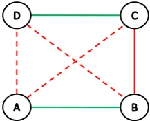
The problem associated with cross-validation, or any eval-uation procedure based on splitting the available informa-tion into training and test partiinforma-tions, can be most easily seen by considering the transitive closure of constraints. Let us consider the available objects and the available constraints (whether given directly or derived from the labels of some objects) as a graph where the data objects are the ver-tices and the constraints are the edges, e.g., with weight 0 (cannot-link) and weight 1 (must-link). The transitive clo-sure provides all edges that can be induced from the given
edges, e.g., if we have, for the objectsA, B, C, D, as
con-straints a must-link(A,B), a must-link(C,D)(green links
in Figure 2), and acannot-link(B,C)(red link in Figure 2),
we can induce the constraintscannot-link(A,C),
cannot-link(A,D), andcannot-link(B,D)(dotted red links in Fig-ure 2). Note that, although the transitive closFig-ure will usu-ally add a considerable number of edges, neither the graph overall nor any small components necessarily become
com-Figure 2: Transitive closure for some given con-straints (example): with given constraints must-link(A,B), must-link(C,D), and cannot-link(B,C), the constraints cannot-link(A,C), cannot-link(A,D), and
cannot-link(B,D)can be induced.
pletely connected. For example, if we had the opposite
con-straints cannot-link(A,B),cannot-link(C,D), and
must-link(B,C), the constraintscannot-link(A,C)and cannot-link(B,D) could be derived, but we would not know
any-thing about(A,D).
We partition the available information into different folds, to use some part for training and some part for testing. The transitive closure of pairwise instance level constraints, whether explicitly computed or not, can lead unintention-ally to the indirect presence of information in some fold or partition. For example, suppose a training fold contains the
constraintsmust-link(A,B)and cannot-link(B,C). If the
test fold contains the constraintcannot-link(A,C), this is
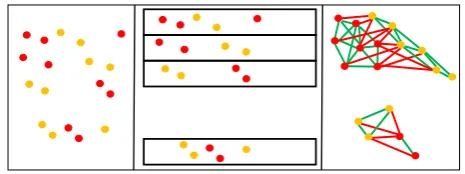
[image:3.595.368.477.279.367.2]Figure 3: Scenario I: Labeled objects are provided. Labeled objects are distributed onn−1training folds and 1 test fold. Constraints are derived from the labeled objects inn−1folds for the training set and from thenth fold for the test set.
in correctly cutting the graph of constraints, to ensure inde-pendence between training and test folds.
3.1.1
Scenario I: Providing Labeled Objects
First consider the simpler and more widely applicable sce-nario where the user provides a certain percentage of labeled objects. This scenario is more widely applicable because, from labeled objects, we can derive instance level pairwise constraints (must-link and cannot-link constraints), and so use algorithms that require labeled objects as input as well as those that require a set of instance level constraints. In our context, this scenario is simpler because we can set up the cross-validation (and, based on that, the model selection framework) based on individual objects and, thus, directly avoid the duplicate use of the same information. This setup of the framework is as follows.
We partition the set of all labeled objects into the desired
numbernof folds (cf. Figure 3). As usual in cross-validation,
one of the folds is left out each time as a test set and the
union of the remainingn−1 folds provides the training set.
Instance level constraints can then be derived from the
la-bels, independently for the training set (n−1 folds together)
and for the test set. When two objects have the same label, this results in a must-link constraint; different labels for two objects result in a cannot-link constraint. If the framework is applied with an algorithm that uses labels directly, then we do not need to derive the constraints for the training set, only for the test set. In either case, only the labels or
con-straints coming from the union of then−1 training folds are
used in the clustering process. For the test fold, constraints are necessarily derived and they will obviously not have any overlap with the information contained in the training folds. Only these constraints are used for the estimation of the classification error for the clustering result.
The procedure is repeated n times, using each of then
folds once as the test fold.
3.1.2
Scenario II: Providing Pairwise Instance-Level
Constraints
If we are directly given a set of (must-link/cannot-link) constraints, we extend this set by computing the
transi-tive closure (e.g., if we have amust-link(A,B)and a
must-link(B,C)we can derive amust-link(A,C)). A straightfor-ward approach of using separated components of the con-straint graph for different partitions could address the issue of ensuring independence between a training fold and test fold; but, first, we are not guaranteed to have separated components, and second, if we were, this would likely result
Figure 4: Scenario II: Pairwise constraints are pro-vided. Objects involved in constraints are dis-tributed onn−1training folds and 1 test fold. Con-straints between objects in the training folds and the test fold are removed. The transitive closure of constraints is computed for all objects in the n−1
training folds for the training set and for the objects in the test fold for the test set.
in an imbalanced distribution of information since separated components are likely to describe different spatial areas of the data. This approach would lead the algorithm to overfit to the provided constraints.
To ensure our cross-validation procedure avoids the pitfall of using the same information for training and testing, we
partition thedata objects involved in any pairwise constraint
in training folds and test fold, thendelete all constraints that
involve an object from the training fold and an object from the test fold. For n-fold cross validation, we partition the
objects intonfolds and use, in turn,n−1 folds as training
set and the remaining fold as test set (cf. Figure 4). This way, when provided with pairwise instance-level constraints, the cross-validation procedure essentially reduces to the ap-proach of Scenario I, where we are given labels.
3.2
Transforming the Evaluation of
Semi-Su-pervised Clustering to Classification
Eval-uation
Regardless of whether the clustering algorithm uses the labels or constraints, we can use the constraints to estimate the quality of a partition produced by the clustering algo-rithm. We can consider a produced partition as a classi-fier that distinguishing the class of must-link (class 1) from cannot-link (class 0) constraints. In other words (and sim-ilar to so-called “pair-counting” cluster evaluation [1]) we evaluate for pairs of objects in the test fold whether their constraint has been “recognized” by the clustering procedure (as opposed to evaluating the performance at an object level where we would consider if a single object is a member of an appropriate cluster in some clustering solution). A given clustering solution provides the basis to assess the degree to which the constraints in the test fold are satisfied or violated. As a consequence, we do not need to resort to some arbitrary clustering evaluation measure, but can use the well estab-lished F-measure to estimate the constraint satisfaction of a given solution.
The semi-supervised clustering problem can then be con-sidered as a classification problem as follows: for each test fold, we have a set of must-link constraints (class 1) and
cannot-link constraints (class 0). The clustering solution
[image:4.595.307.538.85.173.2]and true negative for class 0) or not (false negative for class 1 and false positive for class 0); likewise, pairs of objects that are involved in a cannot-link constraint are either cor-rectly separated in two clusters (true positive for class 0 and true negative for class 1) or paired in the same cluster (false negative for class 0 and false positive for class 1). Based on these numbers, precision and recall, and the F-measure can be computed for each class. The average F-measure for both classes is the criterion for the overall constraint satisfaction of one test fold (see again Figure 1).
3.3
Model Selection
So far, we have noted a possible problem in evaluating semi-supervised clustering based on pairwise constraints when using some partition-based (holdout) evaluation such as cross-validation, and we have elaborated how cross-validation can avoid this problem. Based on this improved formulation of a cross-validation framework for semi-supervised clustering (depending on the nature of the provided data, according to scenario I or scenario II), we can now discuss the process of model selection.
Cross-validation is suitable for estimating the classifica-tion error (here using the F-measure) of a semi-supervised clustering algorithm on some given data set and given labels
or pairwise constraints based on usingntimes a certain
frac-tion of the available informafrac-tion for clustering (n−1
n ) and,
in each case, the remaining fraction (i.e., n1) for evaluation.
The average of the average F-measure over allntest folds is
the criterion for the constraint satisfaction of some cluster model.
Based on this overall error estimation, we can now com-pare the performance of some semi-supervised clustering al-gorithm when using different parameters, i.e., we can com-pare different clustering models. Users who apply this frame-work can now select the best available model for clustering their data. To do so, any algorithm is evaluated in cross-validation for each parameter setting that the user would like to consider, resulting in different cluster models of different quality (as judged based on the estimated classification er-ror, using average F-measure).
Picking the best model based on the error estimate from a cross-validation procedure is still a guess, assuming that the error estimation can be generalized to when complete
information is available. In what follows, we provide an
outline of how well this assumption works for a variety of clustering algorithms applied to different data sets.
4.
EXPERIMENTS
Here we provide a preliminary evaluation of our proposed method for selecting parameters of semi-supervised
cluster-ing methods (calledCVCPfor “Cross-Validation for finding
Clustering Parameters”).
After discussing the experimental setup, we describe two
types of experiments. In Section 4.2 we first argue that
the “internal” (i.e., classification) F-measure values, used to select the best parameters, correlate well with the “external” (i.e., clustering) Overall F-Measure values. Subsequently, in Section 4.3, we report the performance of CVCP compared to the “expected” performance when having to guess the right parameter from the given range.
4.1
Experimental Setup
Semi-Supervised Clustering Methods and Parameters
We apply CVCP using two major representative,semi-super-vised clustering methods, FOSC-OPTICSDend [10] and
MPCKmeans [8], respectively. FOSC-OPTICSDend is a density-based clustering method that requires a parameter
MinPts which specifies the minimum number of points
re-quired in theε-neighborhood of a dense (core) point.
MPCK-means is a variant of K-MPCK-means, and similarly requires a
pa-rameterkthat specifies the number of clusters to be found.
CVCP selects the best parameter values from a range of considered values. These ranges were set as following: For
MinPts, values in [3, 6, 9, 12, 15, 18, 21, 24] were considered, since values in the range between 3 and 24 have been widely used in the literature of density-based clustering for a variety of data sets. Fork, the range of values was set to [2, . . . , M],
whereM is an upper bound for the number of clusters that
a user would reasonably specify for a given data set. For both scenarios — “providing labeled objects” and “pro-viding instance level constraints” — we evaluate the perfor-mance of the semi-supervised clustering algorithms for dif-ferent volumes of information, given in the form of labeled objects and constraints, respectively. For the scenario in which a subset of labeled objects is given, we show the results where labels for 5%, 10%, and 20% of all objects (randomly selected) are given as input to the semi-supervised clustering method. For the scenario in which a subset of constraints is given, we first used the ground truth to generate a candidate “pool” of constraints by randomly selecting 10% of the ob-jects from each class and generating all constraints between these objects. From this pool of constraints, we then ran-domly select subsets of 10%, 20%, and 50% as input to the semi-supervised clustering method.
All reported values are average values computed over 50 independent experiments for each data set, where for each experiment a “new” set of labeled objects or constraints were randomly selected, as described.
Data Sets
For this set of evaluation experiments, we use the following real data sets which exhibit a variety of characteristics in terms of number of objects, number of clusters, and dimen-sionality:
• ALOI: The ALOI data set is acollectionof data sets,
for which we will report average performance. The
collection is based on the Amsterdam Library of Ob-ject Images (ALOI) [15], which stores images of 1000 objects under a variety of viewing angles, illumination angles, and illumination colours. We used image sets that were created by Horta and Campello [17] by
ran-domly selectingkALOI image categories as class labels
100 times for eachk= 2,3,4,5, then sampling
(with-out replacement), each time, 25 images from each of
thek selected categories. So each image collection is
composed of a hundred data sets, of images fromk
cat-egories; each data set has its own set ofk categories.
• UCI: The UC Irvine Machine Learning Repository [3] maintains numerous data sets as a service to the ma-chine learning community. From these data sets, we used the following:
– Iris: This data set contains 3 classes of 50 in-stances each with 4 attributes, where each class contains a type of iris plant and attributes for one instance are the lengths and widths of its sepal and petal. One class is linearly separable from the two which are not linearly separable from each other.
– Wine: This data set contains 178 objects in 13 attributes, with 3 classes. These data are the re-sults of a chemical analysis of wines grown in the same region in Italy but derived from three dif-ferent cultivars.
– Ionosphere: This data set contains 351 instances with 34 continuous attributes, and two classes. The attributes describe radar returns from the ionosphere classified into “good” and “bad” classes (whether they show evidence of some type of struc-ture in the ionosphere or not, respectively).
– Ecoli: The “Ecoli” data set contains 336 objects
in 7 attributes, with 8 classes. Classes in this
data set are protein localization sites in E. coli bacteria.
• ZyeastThis data set is a gene-expression data set re-lated to the Yeast cell cycle. It contains the expression levels of 205 genes (objects) under 20 conditions (at-tributes) with 4 known classes; it was used in [42].
Performance Measure
As our external evaluation measure, we use the “Overall F-Measure” [18]. For a given clustering result, i.e., a par-tition obtained by a clustering method w.r.t. a given pa-rameter value, the Overall F-Measure computes the agree-ment of that partition with the “ground truth” partition as defined by the class labels of the objects. Note, however, that this type of ground truth for clustering results has to be considered with some reservation. For example, the la-bels for the given classes may not correspond to a cluster structure that can be found by a particular clustering al-gorithm/paradigm [14], so we do not expect the absolute F-measure values to be high for all combinations of data sets and clustering methods.
In addition, when computing the Overall F-Measure, we must ensure that the only objects considered are those that are not involved in the constraints given as input to the semi-supervised clustering method (see Section 2).
4.2
Correlation with the External Quality
Measure
Recall that CVCP uses an internal, classification F-measure for the degree of constraint satisfaction in a partition pro-duced by a clustering method, for a particular parameter value. In this subsection, we will show that these internal values of constraint satisfaction quality (based only on the input provided to the semi-supervised clustering algorithm) correlate, in general, very well with the overall quality of the partitions produced by the clustering method for the same parameter values (as measured by the Overall F-Measure
0 5 10 15 20 25
0.2 0.3 0.4 0.5 0.6 0.7 0.8 0.9 1
MinPts
F
-measure
[image:6.595.307.538.85.270.2]CVCP internal classification scores FOSC−OPTICSDend clustering scores
Figure 5: FOSC-OPTICSDend (label scenario) — Curves for a representative data set from ALOI with correlation coefficient=0.9937
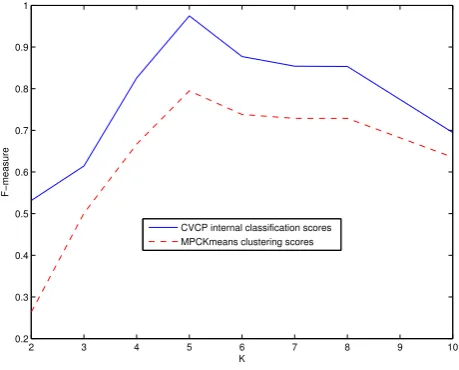
2 3 4 5 6 7 8 9 10
0.2 0.3 0.4 0.5 0.6 0.7 0.8 0.9 1
K
F−measure
CVCP internal classification scores MPCKmeans clustering scores
Figure 6: MPCKmeans (label scenario) — Curves for a representative data set from ALOI with corre-lation coefficient=0.9401
w.r.t. the “ground truth” partition). This means that the in-ternal constraint satisfaction values can, in general, be used to predict the best performing parameter value for a given semi-supervised clustering method.
4.2.1
Providing Labeled Objects
We first show some representative examples of the ex-perimental outcomes of the internal classification scores for different parameters of the semi-supervised clustering meth-ods, using 10% of labeled objects as input. Figure 5 shows the results when using FOSC-OPTICSDend with different
values ofMinPts on one of the ALOI data sets in the ALOI
collection. Figure 6 shows the results when using
MPCK-means with different values of k for the same ALOI data
[image:6.595.308.538.321.506.2]Table 1: FOSC-OPTICSDend (label scenario) — correlation of internal scores with Overall F-Measure
Percent ALOI Iris Wine Ionosphere Ecoli Zyeast
5 0.8019 0.6818 0.9020 0.9177 0.6880 0.9736
10 0.9674 0.6125 0.7880 0.9888 0.8819 0.9433
20 0.9687 0.9902 0.9381 0.9695 0.4570 0.9872
Table 2: MPCKMeans (label scenario) — correla-tion of internal scores with Overall F-Measure
Percent ALOI Iris Wine Ionosphere Ecoli Zyeast
5 0.9661 -0.1643 0.7021 0.5735 0.4360 -0.4847
10 0.9237 0.0062 0.6639 0.4863 -0.0508 -0.7123
[image:7.595.306.539.90.276.2]20 0.9238 -0.3155 0.2282 0.4211 0.1017 -0.7151
Table 1 and Table 2 show the average correlation values (over 50 independent experiments) of internal scores with the corresponding Overall F-Measure scores for different pa-rameter values for FOSC-OPTICSDend and MPCKmeans, respectively. The tables report the average correlation val-ues for all data sets (columns) and for different amounts of labeled objects (rows: 5%, 10%, and 20%) provided as input to the semi-supervised clustering algorithms.
Note that for FOSC-OPTICSDend, the correlation values are overall very high in almost all cases. For MPCKmeans, the results are mixed. For ALOI there is a high correlation with all numbers of provided constraints; for Wine, the cor-relation is high for 5% and 10% of labeled objects, and low for 20% of provided objects; for Ionosphere, the correlation is perhaps “medium” with all numbers of provided constraints; for Iris, and Ecoli, the correlations are generally low; and for Zyeast, the correlation is even strongly negative. The low and negative correlations indicate that MPCKmeans may not represent the most appropriate clustering paradigm for these data sets.
4.2.2
Providing Instance-Level Constraints
As for the “label scenario,” we first show some representa-tive examples of the experimental outcomes that show the internal classification scores for different parameters of the semi-supervised clustering methods, providing 10% of con-straints from the “constraint pool” as input to the algorithm. Figure 7 shows the results when using FOSC-OPTICSDend
with different values ofMinPts, again on one of the ALOI
data sets. Figure 8 shows the results when using
MPCK-means with different values of k for the same ALOI data
set. As in the previous subsection, both figures show the internal classification scores and the clustering score.
As for the results when providing labeled objects, again one can visually determine that in this “constraint scenario” the correlation between the internal classification scores and the Overall F-Measure for clustering is strong.
Table 3 and Table 4 show the average correlation val-ues of internal scores with the corresponding Overall F-Measure values for different parameter values for FOSC-OPTICSDend and MPCKmeans, respectively. The tables report the average correlation values for all data sets (columns) and for different numbers of constraints (from the constraint pool extracted from 10% of labeled objects from each class) provided as input to the semi-supervised clustering algo-rithms (rows: 10%, 20%, and 50%).
As in the label scenario, the correlation values are overall
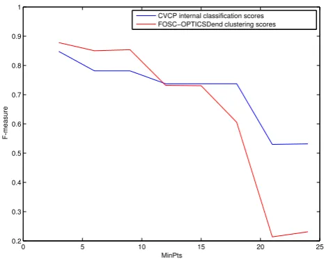
0 5 10 15 20 25
0.2 0.3 0.4 0.5 0.6 0.7 0.8 0.9 1
MinPts
F
-measure
[image:7.595.307.540.335.523.2]CVCP internal classification scores FOSC−OPTICSDend clustering scores
Figure 7: FOSC-OPTICSDend (constraint scenario) — Curves for a representative data set from ALOI with correlation coefficient=0.9784
2 3 4 5 6 7 8 9
0.2 0.3 0.4 0.5 0.6 0.7 0.8 0.9 1
K
F−measure
CVCP internal classification scores MPCKmeans clustering scores
Figure 8: MPCKMeans (constraint scenario) — Curves for a representative data set from ALOI with correlation coefficient=0.9862
Table 3: FOSC-OPTICSDend (constraint scenario) — correlation of internal scores with Overall F-Measure
Percent ALOI Iris Wine Ionosphere Ecoli Zyeast
10 0.8829 0.7696 0.7970 0.9813 0.9450 0.9140
20 0.9013 0.9066 0.8151 0.9881 0.9412 0.9285
50 0.9029 0.8688 0.8034 0.9681 0.8679 0.9081
Table 4: MPCKMeans (constraint scenario) — cor-relation of internal scores with Overall F-Measure
Percent ALOI Iris Wine Ionosphere Ecoli Zyeast
10 0.7755 0.2755 0.2416 0.3021 0.2615 -0.6421
20 0.9256 -0.1921 0.3136 0.5354 0.4875 -0.7290
0.2 0.3 0.4 0.5 0.6 0.7 0.8 0.9 1
[image:8.595.42.282.85.269.2]CVCP−5 Exp−5 CVCP−10 Exp−10 CVCP−20 Exp−20
Figure 9: FOSC-OPTICSDend (label scenario) — Boxplot of the distributions of quality values ob-tained on the ALOI collection, using different per-centages (x) of labeled points as an input, for CVCP (CVCP-x) and expected quality (Exp-x).
very high for FOSC-OPTICSDend in all cases, and mixed for MPCKmeans. As before, the correlation values for MPCK-means are high for ALOI with all numbers of provided con-straints; for Wine, Ionosphere, and Ecoli, the correlation is low to medium for different numbers of provided constraints; and for Iris and Zyeast the correlations are low, and even strongly negative for Zyeast, suggesting the same conclu-sion as before, i.e., that MPCKmeans may not represent the most appropriate clustering paradigm for these data sets.
4.3
Comparison of Clustering Quality
In this section we show how well semi-supervised clus-tering methods perform with the parameter values selected by CVCP. To do so, we report the corresponding Overall F-measure values. We compare this performance, for both semi-supervised clustering methods, with the “expected” per-formance when having to guess the right parameter from the given range. The expected performance is defined as the av-erage Overall F-Measure for the semi-supervised clustering method, measured over all parameter values in the given range from which CVCP selects its value (for this reason, we have conservatively restricted the ranges to be small).
Note that for density-based clustering, there is no existing
heuristic for selecting the parameterMinPts that could be
applied in this context. For convex-shaped clusters, many internal, relative clustering validation criteria have been pro-posed [36]. These measures have been propro-posed for com-pletely unsupervised clustering methods like K-means, and they can be used for model selection in case of MPCK-means. One of the best known and best performing such measures [36] is the Silhouette Coefficient [23], which we also include in the evaluation of MPCKmeans as a baseline, in addition to the expected quality.
4.3.1
Providing Labeled Objects
In this subsection, we show results for the scenario when labeled objects are provided as input to the semi-supervised clustering methods.
0.2 0.3 0.4 0.5 0.6 0.7 0.8 0.9
[image:8.595.295.544.87.265.2]CVCP−5 Exp−5 Sil−5 CVCP−10 Exp−10 Sil−10 CVCP−20 Exp−20 Sil−20
[image:8.595.307.538.383.474.2]Figure 10: MPCKmeans (label scenario) — Boxplot of the distributions of quality values obtained on the ALOI collection, using different percentages (x) of labeled points as an input, for CVCP (CVCP-x), expected quality (Exp-x), and Sihhouette (Sil-x).
Table 5: FOSC-OPTICSDend (label scenario) — av-erage performance using 5 percent of labeled data as an input. 89/100 in ALOI were significant.
Data sets CVCP Expected CVCP Expected
Mean Mean std std
ALOI 0.7489 0.7154 0.0531 0.0039 Iris 0.7251 0.6982 0.0360 0.0042
Wine 0.4659 0.4580 0.0326 0.0049
Ionosphere 0.6036 0.5328 0.0311 0.0063
Ecoli 0.6555 0.6532 0.0192 0.0040
Zyeast 0.9154 0.8946 0.0310 0.0124
Table 6: FOSC-OPTICSDend (label scenario) — av-erage performance using 10 percent of labeled data as an input. 100/100 in ALOI were significant.
Data sets CVCP Expected CVCP Expected
Mean Mean std std
ALOI 0.8485 0.7293 0.0620 0.0071 Iris 0.7615 0.7006 0.0401 0.0066 Wine 0.4717 0.4569 0.0261 0.0161
Ionosphere 0.6189 0.5738 0.0086 0.0065
Ecoli 0.6026 0.5659 0.0723 0.0071
Zyeast 0.9349 0.8939 0.0347 0.0297
Table 7: FOSC-OPTICSDend (label scenario) — av-erage performance using 20 percent of labeled data as an input. 100/100 in ALOI were significant.
Data sets CVCP Expected CVCP Expected
Mean Mean std std
ALOI 0.8569 0.7290 0.0415 0.0106 Iris 0.8251 0.7116 0.0554 0.0126 Wine 0.5569 0.5127 0.0338 0.0191
Ionosphere 0.6228 0.5181 0.0106 0.0088
Ecoli 0.5749 0.5668 0.0202 0.0112
[image:8.595.306.540.523.612.2] [image:8.595.304.539.661.753.2]Table 8: MPCKmeans (label scenario) — average performance using 5 percent of labeled data as an input. 100/100 in ALOI were significant.
Data sets CVCP Exp Silh CVCP Exp Silh
Mean Mean Mean std std std
ALOI 0.7001 0.6250 0.5875 0.0506 0.0045 0.0105
Iris 0.5585 0.5649 0.4456 0.0452 0.0055 0.0057
Wine 0.6523 0.6341 0.3772 0.0416 0.0045 0.0054
Ionosphere 0.6159 0.6119 0.4602 0.0641 0.0051 0.0039
Ecoli 0.4914 0.5025 0.3783 0.0812 0.0037 0.0046
[image:9.595.39.282.256.332.2]Zyeast 0.5055 0.5346 0.5352 0.0469 0.0043 0.0072
Table 9: MPCKmeans (label scenario) — average performance using 10 percent of labeled data as an input. 100/100 in ALOI were significant.
Data sets CVCP Exp Silh CVCP Exp Silh
Mean Mean Mean std std std
ALOI 0.7196 0.6253 0.5876 0.0485 0.0077 0.0103
Iris 0.5475 0.5645 0.4444 0.0492 0.0083 0.0066
Wine 0.6392 0.6334 0.3753 0.0425 0.0073 0.0099
Ionosphere 0.6681 0.6129 0.4601 0.0853 0.0059 0.0054
Ecoli 0.4705 0.5021 0.3785 0.0719 0.0051 0.0063
[image:9.595.40.280.384.461.2]Zyeast 0.4846 0.5347 0.5387 0.0494 0.0056 0.0087
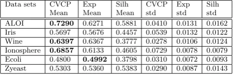
Table 10: MPCKmeans (label scenario) — average performance using 20 percent of labeled data as an input. 100/100 in ALOI were significant.
Data sets CVCP Exp Silh CVCP Exp Silh
Mean Mean Mean std std std
ALOI 0.7290 0.6271 0.5881 0.0410 0.0131 0.0162
Iris 0.5697 0.5676 0.4457 0.0539 0.0132 0.0122
Wine 0.6397 0.6367 0.3777 0.0278 0.0106 0.0124
Ionosphere 0.6857 0.6133 0.4605 0.0729 0.0078 0.0079
Ecoli 0.4800 0.4992 0.3798 0.0310 0.0072 0.0093
Zyeast 0.5303 0.5360 0.5383 0.0290 0.0087 0.0143
Before reporting the average performance for the differ-ent data sets and amounts of labeled objects, we visualize the distributions of the quality values (Overall F-Measure) obtained for the data sets in the ALOI collection, using box-plots.
Figure 9 shows different distributions of quality values for ALOI when using FOSC-OPTICSDend: (1) the quality of FOSC-OPTICSDend when using the value for parameter
MinPtsselected by CVCP, for different percentagesxof
la-beled objects as input, denoted as CVCP-x in the figure;
(2) theexpected quality of FOSC-OPTICSDend when
hav-ing to guess the value for the parameter MinPts, denoted
analogously asExp-x in the figure. One can clearly see that
selecting the parameter value MinPts using CVCP gives a
much better performance in general than the expected per-formance when one has to randomly select the parameter value from the given range. This is true for every amount of used labeled objects, but the difference is more pronounced when using larger numbers of labeled objects.
Figure 10 shows similarly the distribution of quality val-ues on ALOI when using MPCKmeans: (1) the quality of
MPCKmeans when using the value for parameterkselected
by CVCP, (2) the expected quality, and (3) the quality
ob-tained when selecting the parameter value for k that has
the best Silhouette Coefficient. Using Silhouette Coefficient leads to better quality than the expected quality, but CVCP
gives even better quality than the Silhouette Coefficient, for all amounts of labeled objects used. For MPCKmeans, we see again the effect that the quality improves when using larger numbers of labeled objects as input. The absolute F-measure values are overall at a lower level for MPCKmeans than for FOSC-OPTICSDend.
Tables 5, 6, and 7 report the average performance on all data sets when using FOSC-OPTICSDend, for 5%, 10%, and 20% of labeled objects, respectively. The values shown are the mean and the standard deviation of the performance
when selectingMinPtsusing CVCP, and the mean and
stan-dard deviation of the expected performance (computed over 50 experiments).
Tables 8, 9, and 10 report similarly the average perfor-mance on all data sets when using MPCKmeans, for 5%, 10%, and 20% of labeled objects, respectively. For MPCK-means we show in addition to the mean and standard
de-viation of the performance when selecting k using CVCP,
and the expected performance, also the performance when
selectingkusing Silhouette Coefficient.
In all tables, we show the best mean performance for a data set in bold, if the difference to the other mean perfor-mance results is statistically significant at theα= 0.05 level, using a paired t-test. For the ALOI data set collection, we did the test for each of the 100 data sets in the collection separately; the number of data sets for which a difference was statistically significant is given in the table captions.
One can observe that for the semi-supervised, density-based clustering approach FOSC-OPTICSDend, CVCP leads consistently to a much better performance than the expected performance. The difference is statistically significant in al-most all cases, except for Wine and Ecoli when only 5% of la-beled objects are used as input for FOSC-OPTICSDend. For MPCKmeans, CVCP outperforms expected performance and Silhouette significantly for ALOI, Wind, Ionosphere, and Ecoli when using 10% or 20% of labeled objects. When using 5% of labeled objects, the difference in performance for Iris and Ionosphere are not statistically significant, and for Ecoli the expected performance is slightly better than CVCP, and because of very small variance in fact statistically signifi-cant. For Zyeast, Silhouette leads to the best MPCKmeans performance. We observe furthermore, that for all data sets except Wine, the density-based clustering paradigm seems to produce much better clustering results, indicated by much higher Overall F-Measure values. The results also suggest that CVCP outperforms the other methods in cases when the overall clustering quality can be high, indicating that in cases when no good parameter exists that can lead to a good clustering result, the selection of the “best” value by CVCP can not be significantly better than other methods. This is the case for several data set when using MPCKmeans. (Re-call also that it has been observed before that class labels may not correspond to a cluster structure that can be found by a particular clustering algorithm/paradigm [14].)
4.3.2
Providing Instance-Level Constraints
In this subsection, we show results for the scenario when constraints are provided directly as input to the semi-supervised clustering methods.
Again, we show first a boxplot of the distribution of the quality values obtained for the data sets in ALOI.
0.4 0.5 0.6 0.7 0.8 0.9 1
[image:10.595.42.280.85.268.2]cvcp−5 Exp−5 cvcp−10 Exp−10 cvcp−20 Exp−20
Figure 11: FOSC-OPTICSDend (constraint sce-nario) — Boxplot of the distributions of quality val-ues obtained on the ALOI collection, using different percentages (x) of constraints from the constraint pool as an input, for CVCP (CVCP-x) and expected quality (Exp-x).
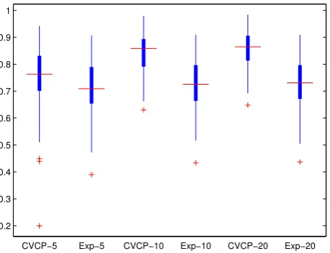
0.2 0.3 0.4 0.5 0.6 0.7 0.8 0.9
[image:10.595.304.539.138.230.2]cvcp−5 Exp−5 Sil−5 cvcp−10 Exp−10 Sil−10 cvcp−20 Exp−20 Sil−20
[image:10.595.305.539.290.384.2]Figure 12: MPCKmeans (constraint scenario) — Boxplot of the distributions of quality values ob-tained on the ALOI collection, using different per-centages (x) of constraints from the constraint pool as input, for CVCP (CVCP-x), expected quality (Exp-x), and Sihhouette (Sil-x).
Table 11: FOSC-OPTICSDend (constraint scenario) — average performance using 10 percent of con-straints from the constraint pool as an input. 97/100 in ALOI were significant.
Data sets CVCP Expected CVCP Expected
Mean Mean std std
ALOI 0.8205 0.7230 0.0674 0.0115 Iris 0.8541 0.7483 0.0489 0.0261 Wine 0.6139 0.5469 0.0446 0.0333
Ionosphere 0.5969 0.5003 0.0264 0.0096
Ecoli 0.5977 0.5376 0.0267 0.0270
Zyeast 0.9586 0.8923 0.0301 0.0286
Table 12: FOSC-OPTICSDend (constraint scenario) — average performance using 20 percent of con-straints from the constraint pool as an input. 99/100 in ALOI were significant.
Data sets CVCP Expected CVCP Expected
Mean Mean std std
ALOI 0.8462 0.7209 0.0547 0.0120 Iris 0.8606 0.7391 0.0446 0.0279 Wine 0.6165 0.5529 0.0415 0.0361
Ionosphere 0.6116 0.5212 0.0136 0.0054
Ecoli 0.6443 0.5955 0.0624 0.0492
Zyeast 0.9705 0.8974 0.0131 0.0033
Table 13: FOSC-OPTICSDend (constraint scenario) — average performance using 50 percent of con-straints from the constraint pool as an input. 99/100 in ALOI were significant.
Data sets CVCP Expected CVCP Expected
Mean Mean std std
ALOI 0.8523 0.7234 0.0445 0.0106 Iris 0.8833 0.7502 0.0160 0.0239 Wine 0.5760 0.5249 0.0604 0.0494
Ionosphere 0.6088 0.5191 0.0172 0.0045
Ecoli 0.6016 0.5584 0.0318 0.0355
[image:10.595.41.278.349.526.2]Zyeast 0.9698 0.8981 0.0160 0.0030
Table 14: MPCKmeans (constraint scenario) — av-erage performance using 10 percent of constraints from the constraint pool as an input. 94/100 in ALOI were significant.
Data sets CVCP Exp Silh CVCP Exp Silh
Mean Mean Mean std std std
ALOI 0.7267 0.6286 0.5967 0.0630 0.0050 0.0061
Iris 0.5918 0.5676 0.4445 0.0706 0.0065 0.0054
Wine 0.6357 0.6444 0.3808 0.0376 0.0037 0.0037
Ionosphere 0.6955 0.6095 0.4618 0.0467 0.0028 0.0020
Ecoli 0.4854 0.5059 0.3796 0.1021 0.0027 0.0043
Zyeast 0.5214 0.5257 0.5377 0.0375 0.0026 0.0051
shows different distributions of quality values on ALOI when
using MPCKmeans, for different percentagesxof used
con-straints. As before, we show the performance of CVCP as well as the expected performance, and for MPCKmeans the
performance when selectingk via Silhouette Coefficient.
The results are very similar to the results obtained in the scenario when labeled objects are provided, leading to the same conclusions for the ALOI data collection: using CVCP
to select MinPts for FOSC-OPTICSDend gives much
bet-ter performance than the expected performance, and using
CVCP to selectk for MPCKmeans give much better than
both the expected performance and the performance using Silhouette Coefficient. And, again, we can observe that the results improve when using larger numbers of constraints as input (more so for FOSC-OPTICSDend than for MPCK-means), and that the absolute F-measure values are overall at a lower level for MPCKmeans.
[image:10.595.303.542.444.523.2] [image:10.595.44.276.662.752.2]Table 15: MPCKmeans (constraint scenario) — av-erage performance using 20 percent of constraints from the constraint pool as an input. 96/100 in ALOI were significant.
Data sets CVCP Exp Silh CVCP Exp Silh
Mean Mean Mean std std std
ALOI 0.7295 0.6202 0.5815 0.0491 0.0052 0.0060
Iris 0.5991 0.5644 0.4442 0.0072 0.0056 0.0049
Wine 0.6395 0.6452 0.3768 0.0052 0.0027 0.0034
Ionosphere 0.7082 0.6088 0.4594 0.0228 0.0030 0.0027
Ecoli 0.5151 0.5079 0.3835 0.0993 0.0031 0.0044
[image:11.595.41.282.275.354.2]Zyeast 0.5233 0.5210 0.5351 0.0330 0.0030 0.0048
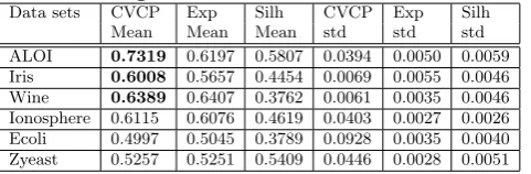
Table 16: MPCKmeans (constraint scenario) — av-erage performance using 50 percent of constraints from the constraint pool as an input. 97/100 in ALOI were significant.
Data sets CVCP Exp Silh CVCP Exp Silh
Mean Mean Mean std std std
ALOI 0.7319 0.6197 0.5807 0.0394 0.0050 0.0059
Iris 0.6008 0.5657 0.4454 0.0069 0.0055 0.0046
Wine 0.6389 0.6407 0.3762 0.0061 0.0035 0.0046
Ionosphere 0.6115 0.6076 0.4619 0.0403 0.0027 0.0026
Ecoli 0.4997 0.5045 0.3789 0.0928 0.0035 0.0040
Zyeast 0.5257 0.5251 0.5409 0.0446 0.0028 0.0051
Again, the values shown are the mean and the standard
deviation of the performance when selectingM inP tsusing
CVCP, and the mean and standard deviation of the expected performance (over 50 experiments).
Tables 14, 15, and 16 report similarly the average per-formance on all data sets for MPCKmeans, including the
performance when selectingkusing Silhouette Coefficient.
The results for the constraint scenario are very similar to those for the label scenario, giving the same overall pic-ture that CVCP is very effective in selecting a good pa-rameter value for semi-supervised clustering methods. The performance is, in general (except for some MPCKmeans results), significantly improved compared to the expected performance and compared to using Silhouette (for MPCK-means).
5.
CONCLUSION
We have proposed a model selection method, CVCP, for semi-supervised clustering, based on a sound cross-validation procedure that uses given input constraints within the semi-supervised clustering algorithm (either explicitly or implic-itly as as set of labeled objects). The method automatically finds the most appropriate clustering parameter values (e.g., number of clusters, density-parameters), which are normally determined manually. The method is described in detail, and an extensive experimental evaluation has confirmed the effectiveness of the proposed method.
Future work will include the study of CVCP in combi-nation with other semi-supervised clustering methods, and an investigation of how our approach could be extended to compare and select alternative clustering methods.
Acknowledgements. This project was partially funded by NSERC (Canada), FAPESP (Brazil), and CNPq (Brazil).
6.
REFERENCES
[1] E. Achtert, S. Goldhofer, H.-P. Kriegel, E. Schubert, and A. Zimek. Evaluation of clusterings – metrics and
visual support. InProceedings of the 28th
International Conference on Data Engineering (ICDE), Washington, DC, pages 1285–1288, 2012.
[2] M. R. Anderberg.Cluster Analysis for Applications.
Academic Press, 1973.
[3] K. Bache and M. Lichman. UCI machine learning repository, 2013.
[4] S. Basu, A. Banerjee, and R. J. Mooney. Active semi-supervision for pairwise constrained clustering. In
Proceedings of the 4th SIAM International Conference on Data Mining (SDM), Lake Buena Vista, FL, 2004. [5] S. Basu, M. Bilenko, and R. J. Mooney. A
probabilistic framework for semi-supervised clustering. InProceedings of the 10th ACM International
Conference on Knowledge Discovery and Data Mining (SIGKDD), Seattle, WA, pages 59–68, 2004.
[6] S. Basu, I. Davidson, and K. Wagstaff, editors.
Constraint Clustering: Advances in Algorithms, Applications and Theory. CRC Press, Boca Raton, London, New York, 2008.
[7] P. Berkhin. A survey of clustering data mining techniques. In J. Kogan, C. Nicholas, and M. Teboulle,
editors,Grouping Multidimensional Data: Recent
Advances in Clustering. Springer, 2006.
[8] M. Bilenko, S. Basu, and R. J. Mooney. Integrating constraints and metric learning in semi-supervised
clustering. InProceedings of the 21st International
Conference on Machine Learning (ICML), Banff, AB, Canada, 2004.
[9] C. B¨ohm and C. Plant. HISSCLU: a hierarchical
density-based method for semi-supervised clustering. InProceedings of the 11th International Conference on Extending Database Technology (EDBT), Nantes, France, pages 440–451, 2008.
[10] R. J. G. B. Campello, D. Moulavi, A. Zimek, and J. Sander. A framework for semi-supervised and unsupervised optimal extraction of clusters from
hierarchies.Data Mining and Knowledge Discovery,
27(3):344–371, 2013.
[11] I. Davidson and S. S. Ravi. The complexity of non-hierarchical clustering with instance and cluster
level constraints.Data Mining and Knowledge
Discovery, 14(1):25–61, 2007.
[12] I. Davidson, K. L. Wagstaff, and S. Basu. Measuring constraint-set utility for partitional clustering
algorithms. InProceedings of the 10th European
Conference on Principles and Practice of Knowledge Discovery in Databases (PKDD), Berlin, Germany, pages 115–126, 2006.
[13] B. S. Everitt, S. Landau, and M. Leese.Cluster
Analysis. Arnold, 4th edition, 2001.
[14] I. F¨arber, S. G¨unnemann, H.-P. Kriegel, P. Kr¨oger,
E. M¨uller, E. Schubert, T. Seidl, and A. Zimek. On
using class-labels in evaluation of clusterings. In
MultiClust: 1st International Workshop on Discovering, Summarizing and Using Multiple Clusterings Held in Conjunction with KDD 2010, Washington, DC, 2010.
Smeulders. The Amsterdam Library of Object Images.
International Journal of Computer Vision, 61(1):103–112, 2005.
[16] J. A. Hartigan.Clustering Algorithms. John
Wiley&Sons, New York, London, Sydney, Toronto, 1975.
[17] D. Horta and R. J. G. B. Campello. Automatic aspect
discrimination in data clustering.Pattern Recognition,
45(12):4370–4388, 2012.
[18] L. Hubert and P. Arabie. Comparing partitions.
Journal of Classification, 2(1):193–218, 1985.
[19] A. K. Jain. Data clustering: 50 years beyond k-means.
Pattern Recognition Letters, 31:651–666, 2010.
[20] A. K. Jain and R. C. Dubes.Algorithms for Clustering
Data. Prentice Hall, Englewood Cliffs, 1988.
[21] A. K. Jain, M. N. Murty, and P. J. Flynn. Data
clustering: A review.ACM Computing Surveys,
31(3):264–323, 1999.
[22] D. Jiang, C. Tang, and A. Zhang. Cluster analysis for
gene expression data: A survey.IEEE Transactions on
Knowledge and Data Engineering, 16(11):1370–1386, 2004.
[23] L. Kaufman and P. J. Rousseeuw.Finding Groups in
Data: An Introduction to Cluster Analyis. John Wiley&Sons, 1990.
[24] H. A. Kestler, J. M. Kraus, G. Palm, and F. Schwenker. On the effects of constraints in
semi-supervised hierarchical clustering. InProceedings
of the Second IAPR Workshop Artificial Neural Networks in Pattern Recognition (ANNPR), Ulm, Germany, 2006.
[25] D. Klein, S. D. Kamvar, and C. D. Manning. From instance-level constraints to space-level constraints: Making the most of prior knowledge in data
clustering. InProceedings of the 19th International
Conference on Machine Learning (ICML), Sydney, Australia, pages 307–314, 2002.
[26] H.-P. Kriegel, P. Kr¨oger, J. Sander, and A. Zimek.
Density-based clustering.Wiley Interdisciplinary
Reviews: Data Mining and Knowledge Discovery, 1(3):231–240, 2011.
[27] M. H. C. Law, A. Topchy, and A. K. Jain. Clustering
with soft and group constraints. InJoint IAPR
International Workshops on Structural, Syntactic, and Statistical Pattern Recognition (SSPR and SPR), Lisbon, Portugal, pages 662–670, 2004.
[28] L. Lelis and J. Sander. Semi-supervised density-based
clustering. InProceedings of the 9th IEEE
International Conference on Data Mining (ICDM), Miami, FL, pages 842–847, 2009.
[29] P. Li, Y. Ying, and C. Campbell. A variational
approach to semi-supervised clustering. InProceedings
of the 17th European Symposium on Artificial Neural Networks (ESANN), Bruges, Belgium, 2009.
[30] G. W. Milligan and M. C. Cooper. An examination
of procedures for determining the number of clusters
in a data set.Psychometrika, 50(2):159–179, 1985.
[31] C. Ruiz, M. Spiliopoulou, and E. Menasalvas. C-DBSCAN: Density-based clustering with constraints. In A. An, J. Stefanowski, S. Ramanna,
C. Butz, W. Pedrycz, and G. Wang, editors,Rough
Sets, Fuzzy Sets, Data Mining and Granular Computing, pages 216–223. 2007.
[32] C. Ruiz, M. Spiliopoulou, and E. Menasalvas.
Density-based semi-supervised clustering.Data Mining
and Knowledge Discovery, 21(3):345–370, 2010. [33] A. Silva and C. Antunes. Semi-supervised clustering:
A case study. InProceedings of the 8th International
Conference on Machine Learning and Data Mining in Pattern Recognition (MLDM), Berlin, Germany, pages 252–263, 2012.
[34] K. Sim, V. Gopalkrishnan, A. Zimek, and G. Cong. A
survey on enhanced subspace clustering.Data Mining
and Knowledge Discovery, 26(2):332–397, 2013. [35] A. G. Skarmeta, A. Bensaid, and N. Tazi. Data
mining for text categorization with semi-supervised
agglomerative hierarchical clustering.International
Journal of Intelligent Systems, 15(7):633–646, 2000. [36] L. Vendramin, R. J. G. B. Campello, and E. R.
Hruschka. Relative clustering validity criteria: A
comparative overview.Statistical Analysis and Data
Mining, 3(4):209–235, 2010.
[37] K. Wagstaff and C. Cardie. Clustering with
instance-level constraints. InProceedings of the 17th
International Conference on Machine Learning (ICML), Stanford University, CA, pages 1103–1110, 2000.
[38] K. Wagstaff, C. Cardie, S. Rogers, and S. Schr¨odl.
Constrained k-means clustering with background
knowledge. InProceedings of the 18th International
Conference on Machine Learning (ICML), Williams College, MA, pages 577–584, 2001.
[39] K. L. Wagstaff.Intelligent Clustering with
Instance-Level Constraints. PhD thesis, Department of Computer Science, Cornell University, 2002.
[40] L. Wu, S. C. H. Hoi, R. Jin, J. Zhu, and N. Yu. Learning bregman distance functions for
semi-supervised clustering.IEEE Transactions on
Knowledge and Data Engineering, 24(3):478–491, 2012.
[41] R. Xu and D. Wunsch II. Survey of clustering
algorithms.IEEE Transactions on Neural Networks,
16:645–678, 2005.
[42] K. Y. Yeung, M. Medvedovic, and R. E. Bumgarner. Clustering gene-expression data with repeated
measurements.Genome Biology, 4(5), 2003.
[43] L. Zheng and T. Li. Semi-supervised hierarchical
clustering. InProceedings of the 11th IEEE