This is a repository copy of
Crystallisation route map
.
White Rose Research Online URL for this paper:
http://eprints.whiterose.ac.uk/120448/
Version: Accepted Version
Book Section:
Camacho Corzo, DM, Ma, CY orcid.org/0000-0002-4576-7411, Ramachandran, V et al. (2
more authors) (2017) Crystallisation route map. In: NATO Science for Peace and Security
Series A: Chemistry and Biology. NATO Science for Peace and Security Series A:
Chemistry and Biology . Springer , Dordrecht , pp. 179-213. ISBN 978-94-024-1115-7
https://doi.org/10.1007/978-94-024-1117-1_11
[email protected] https://eprints.whiterose.ac.uk/ Reuse
Unless indicated otherwise, fulltext items are protected by copyright with all rights reserved. The copyright exception in section 29 of the Copyright, Designs and Patents Act 1988 allows the making of a single copy solely for the purpose of non-commercial research or private study within the limits of fair dealing. The publisher or other rights-holder may allow further reproduction and re-use of this version - refer to the White Rose Research Online record for this item. Where records identify the publisher as the copyright holder, users can verify any specific terms of use on the publisher’s website.
Takedown
If you consider content in White Rose Research Online to be in breach of UK law, please notify us by
Chapter 11
Crystallisation Route Map
Diana M. Camacho Corzo, Cai Y. Ma, Vasuki Ramachandran, Tariq Mahmud and
Kevin J. Roberts
Abstract A route map for the assessment of crystallisation processes is presented. A theoretical
background on solubility, meta-stable zone width, nucleation and crystal growth kinetics is presented with practical examples. The concepts of crystallisation hydrodynamics and the application of population balances and computational fluid dynamics for modelling crystallisation processes and their scaling up are also covered.
Keywords Solubility, Supersaturation, Critical Undercooling, Metastable Zone Width (MSZW),
Introduction
Crystallisation is a key process used in the manufacture of drugs, pharmaceuticals and fine chemicals which enables e.g. the separation and purification of particulate materials. In some cases crystallisation needs to be avoided, e.g. fuels operating in cold weather or within drugs stabilised in highly concentrated liquid-formulations. Compared with other techniques, such as distillation crystallization it is a more energy-efficient process involving lower temperatures, which are more appropriate for processing heat-sensitive chemical products. The crystallisation process is driven by supersaturation and this affects solid-liquid separation and product purification
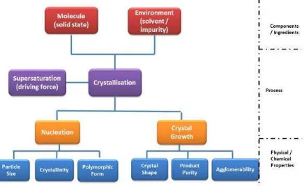
Fig. 1 A schematic showing the role played by the fundamental parameters of crystallisation (nucleation and
growth) in directing the physical properties of the resulting solid forms. Prediction of the outcomes would allow greater control of the final product
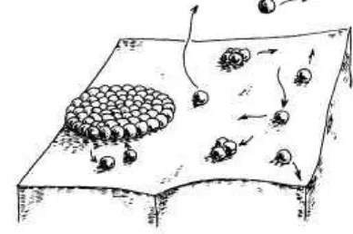
The fundamental concepts related to a crystallisation process involve two key stages viz: nucleation, which is three dimensional (3D) (assembly of molecular clusters on nm size scale) and growth which is two dimensional (2D) (on all atomically smooth particle surfaces) as shown in the schematic in Fig.
1. Nucleation will have an impact on the particles’ size, crystallinity and the polymorphic form
obtained, whilst crystal growth will have a direct impact on the shape of the final crystals, their purity and agglomerability.
Solubility
Solubility and the van’t Hoff Plot
When excess solid is mixed with a solvent at a constant temperature, the solid will dissolve until equilibrium is established. The resulting solution is said to be saturated and the composition of the solution is the equilibrium solubility. The most common ways of expressing solubility are: mass of
[image:3.595.84.520.200.467.2]If the solute-solute interactions in the solid are the same as the solute-solvent interactions the only enthalpy change involved is the enthalpy of fusion. Based on this, the ideal solubility can be predicted using the Hildebrand equation:
(1)
where
= enthalpy of fusion of pure solute = fusion temperature of pure solute = gas constant
= temperature
Since Hf = Tf Sf this can also be rewritten as:
(2)
where = entropy of fusion of pure solute.
In a non-ideal solution the Hildebrand equation neglects the enthalpy and entropy of mixing. This
effect can be included by replacing by (the enthalpy of dissolution) and by (the
entropy of dissolution) yielding the van´t Hoff equation [1, 2]:
(3)
A plot of ln versus expected to yield a straight line with a gradient of and an intercept of
.
Understanding Solution Structure
A plot of the solubility and the solution´s ideality in the same plane of coordinates can give an indication of the strength of the solution´s molecular interactions. The difference between the two
lines will give the activity coefficient at saturation . ideal solution, less than ideal and
more than ideal. Figure 2, after [3], shows the ideal and experimental solubility for succinic acid in water and isopropanol. In water solubility is greater than ideal solubility, i.e. solute-solvent
interactions are enhanced. In isopropanol solubility is lower than ideal, i.e. solute –solute interactions
are enhanced [1, 2].
Solute-solvent interactions
[image:4.595.256.499.586.774.2]Solute-solute interactions
Fig. 2 Ideal and experimental
Supersaturation and Metastable Zone Width
Supersaturation
The extent to which a solution exceeds equilibrium solubility can be expressed either by supersaturation ratio or relative supersaturation as given below [4].
(4)
(5)
where is the solution concentration and is the equilibrium concentration.
Metastable Zone Width (MSZW)
The temperature-concentration diagram can be divided into three regions (stable, metastable and labile) [4] as shown in Fig. 3. As cooling rate increases, so does supersaturation and nucleation rate but the nucleation cluster size and particle size decrease. In extreme cases at very high supersaturations when the cluster size is the same as the molecular size, an amorphous phase instead of crystalline solid will be obtained.
Fig. 3 (a) Schematic of solubility-supersolubility; (b) Meta stable zone width is wider and crystal size decreases
as the cooling rate increases
In the stable region, the solution is undersaturated and there is no possibility of crystallisation and this
region is represented by a point A at temperature TA. When the temperature is reduced to TB, the
solution is at equilibrium (represented by point B on the schematic). TB is the dissolution temperature
where the solute particles are completely dissolved and the solution cannot take any more solid particles. The region between the equilibrium curve and the broken line is called the metastable zone. In this region, represented by point C at temperature , the solution is saturated and can remain in this state for long periods without spontaneous crystallisation if not disturbed.
The metastable zone width (MSZW) can be defined as the difference between the maximum solution
concentration in the supersaturated state before crystallisation takes place and the solution
concentration at equilibrium
Co
n
c
e
n
tr
a
ti
o
n
,
C
Temperature, T metastable zone
undersaturated labile region
CA
TA A B C
TB TC D
TD
equilibrium solubility curve
C
o
n
ce
n
tratio
n
,
C
Temperature, T
undersaturated CA
T Crystallization line
[image:5.595.74.512.385.567.2](6)
MSZW can be defined in terms of undercooling as the difference between dissolution temperature
and crystallisation temperature .
(7)
The relationship between supersaturation and undercooling is given by:
(8)
The third region above the metastable zone is the labile region (represented by the point D at
temperature, TD) and in this region precipitation is almost instantaneous.
Nucleation Kinetics
Classical Nucleation Theory (CNT)
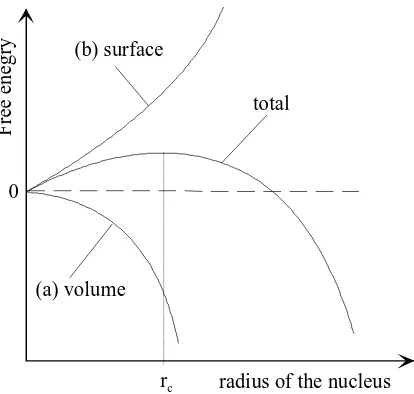
Nucleation refers to the step in which individual solute molecules (or atoms) that are dispersed in the solvent structure will begin to cluster together. Some of these clusters may grow sufficiently large to form stable nuclei and subsequently form crystals. Nucleation is best understood by examining the free energy changes associated with nucleus formation. The volume effect on the free energy of a nucleus is associated with the decrease in free energy per molecule, when the molecule is transferred
from the supersaturated solution to the solid phase, and has an dependence (Fig. 4). The surface of
the new solid phase has an energy associated with it and this results in an increase of free energy per
unit surface area of the cluster which has an dependence. The sum of these two contribution yields
the total free energy. As the total free energy has to decrease for the spontaneous process to take place, large nuclei will be favoured during the process due to their lower free energy. A nucleus that achieves
a size greater than the critical radius will grow into a crystal [4].
The critical radius for the case of a spherical 3D nucleus is given by:
(9)
where: = surface energy
= molecular volume =Boltzmann constant = Temperature = supersaturation
decreases with increasing so nucleation becomes easier and the nucleation rate, J, is given by:
(10)
Methods to Study Nucleation: Polythermal Method
Nucleation can be studied by measuring the turbidity of a crystallising solution by either polythermal or isothermal methods. As nuclei form and grow in an originally clear solution, the optical transmittance of the medium decreases. The polythermal method is based on the determination of the MSZW and the effect exerted on it by the rate at which supersaturation is created. The isothermal
method is based on determination of induction time i.e. the time taken for crystallisation to be
detected at constant temperature and the influence of the supersaturation on this time.
In polythermal method, as shown in Fig. 5, the difference between the dissolution temperature
and the crystallisation temperature is measured as a function of cooling rate . Polythermal
experimental data can be analysed using different approaches:
Polythermal Method
Ny´vlt Approach
Ny´vlt approach [5, 6] uses an empirical expression for nucleation rate:
(11)
where is an empirical parameter of nucleation rate and is related to by Eq. 12:
(12)
(13)
The slope of a linear fit of experimental polythermal data in versus coordinates will deliver
the order of nucleation .
Fr
ee
en
eg
ry
radius of the nucleus rc
(b) surface
(a) volume
total
[image:7.595.249.456.68.265.2]0
Fig. 4 Change in free energy as a
KBHR Approach
The KBHR approach [8-11] uses the expression of CNT defined in terms of relative critical
undercooling given by:
(14)
Where is the solution equilibrium temperature.
The slope of a linear fit of experimental polythermal data according to the expression
will deliver the mechanism ruling the crystallisation process as defined by the rule of three (Fig. 6)
Fig. 6 Assessment of nucleation mechanism from polythermal data using the KBHR model (Reproduced by
consent of CrystEngComm from [10])
Further fitting of the data to specific models related to each case of nucleation allows determining interfacial tensions and nucleation rates in the case of progressive nucleation (PN) or the concentration
of nuclei at the nucleation point in the case of instantaneous nucleation (IN).
RULE OF THREE
Slope <3
Yes No
INSTANTANEOUS NUCLEATION (IN)
[image:8.595.276.433.66.256.2]PROGRESSIVE NUCLEATION (PN) Fig. 5 Transmittance versus
[image:8.595.72.484.458.672.2]Progressive Nucleation [9]: where new crystal nuclei are continuously formed in the presence of the already growing ones.
(15)
Here the three free parameters , and are given by
(16)
(17)
(18)
where is the number of crystals at the detection point, is the volume of the solution and is
defined by
(19)
In this expression is the nucleus shape factor, volume occupied by a solute molecule in the
crystal and is the molecular latent heat of crystallisation.
Instantaneous Nucleation [8]: where all nuclei emerge at once at the beginning of the crystallisation
process to subsequently grow and develop into crystal.
ln (20)
with given by
(21)
where is the relative critical undercooling at the IN point, and are the growth exponents, is
the dimensionality of crystal growth, is the relative volume of crystals at the detection point,
is the growth rate constant, is the crystal shape factor and is defined by
(22)
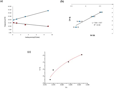
Examples of the polythermal method applied to the case of -para-aminobenzoic acid ( -PABA)
crystallising from ethanol [12] and methyl stearate crystallising from kerosene [10] are presented
below. Using the KBHR approach, the analysis of the crystallisation process for -PABA solutions
showed that crystals are formed by means of IN (Fig. 7). The concentration of PABA nuclei C0 at the
nucleation point, for different solution concentrations, was found to be in the order of 6.6 x 10⁸– 1.3 X
Fig. 7 Example of application KBHR approach to the analysis of polythermal data collected for -PABA crystallising from ethanol with concentration (170 g/Kg). (a) Crystallisation and dissolution temperatures as a
function of cooling rate (b) Plot of vs (Reproduced by consent of Faraday Discussions from [12])
[image:10.595.116.481.76.223.2]In contrast, the example of methyl stearate crystallising from kerosene (Fig. 8) reveals a PN nucleation mechanism.
Fig. 8 Example of application KBHR approach to the analysis of polythermal data collected for methyl stearate
crystallising from kerosene with concentration (250 gr/l) (a) Crystallisation and dissolution temperatures as a
function of cooling rate (b) Plot of vs (c) Plot of vs (Reproduced by consent of
CrystEngComm from [10])
In this case the application of the methodology to different solution concentrations allowed obtaining
interfacial tensions , critical radius and nucleation rates in the range of 1.21 - 1.91 mJ m2,
0.7-0.9 nm and 5.1 1016 -7.9 1016 nuclei ml-1 s-1, respectively.
0.5 0.6 0.7 0.8 0.9 1 1.1 1.2 1.3 1.4 1.5 1.6 1.7 -5.00 5.00 15.00 25.00 35.00 45.00 55.00
0 0.2 0.4 0.6 0.8 1 1.2
S u p e rs a tu ra ti o n r a ti o ( S ) T e m p e ra tu re ( ° C )
Cooling Rate (q) (°C/min)
y = 1.63x - 0.77 R² = 0.98
-7 -6.5 -6 -5.5 -5 -4.5 -4 -3.5 -3 -3.9 -3.4 -2.9 -2.4 -1.9
ln
q
ln uc
0.00 5.00 10.00 15.00 20.00 25.00 30.00 35.00 40.00
0 2 4 6 8 10
T e m p e ra tu re ( º C )
Cooling rate (q) (ºC/min)
y = 3.6x + 10.7 R² = 0.93
-7 -6 -5 -4 -3 -2 -1 0
-4.5 -4 -3.5 -3
Ln
q
ln Uc
0.010 0.015 0.020 0.025 0.030 0.035 -6 -5 -4 -3 -2 L n q Uc
(a) (b)
(b) (a)
[image:10.595.97.496.323.637.2]Methods to Study Nucleation: Isothermal Method
In the isothermal method as shown in Fig. 9, a solution is crash cooled to different temperatures within the MSZW and the induction time is monitored by the change in the solution tubidity, from the time at which the solution reached the predetermined temperature to that of the crystallisation onset, which corresponds to the time at which the light transmittance decreases [11, 13].
The interfacial tension can be calculated from the slope of the line of a plot of experimental data in
versus according to the expression below
ln ln (23)
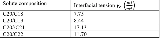
The plots obtained by application of isothermal method for n-eicosane crystallising from n-dodecane solvent in the presence of different impurities [14] are given in Fig. 10. The corresponding interfacial
tensions obtained according to Eq. (23) are given in Table 1.
Table 1 Interfacial tensions obtained by the application of the isothermal method for n-eicosane (C20)
crystallising from n-dodecane in the presence of different impurities [14]
Solute composition Interfacial tension
C20/C18 7.75
C20/C19 8.44
C20//C21 17.13
[image:11.595.236.468.151.319.2]C20/C22 11.70
Fig. 9 Turbidity profile of a
[image:11.595.151.454.500.649.2]solution crystallising at a fixed temperature
Fig. 10 Plot of versus for n-eicosane (C20) crystallising from n-dodecane
in the presence of different impurities. ()
[image:11.595.158.439.698.765.2]Crystal Growth Kinetics
The second step in a crystallisation process is the growth of stable nuclei into crystals. This process can occur through different mechanisms in each of the crystal faces.
Birth and Spread (B&S) Model
This involves the formation of a stable cluster of molecules on a flat face (Fig. 11), i.e. nucleation is required. As for 3D nucleation, the 2D nucleus must reach a critical radius to become stable [4, 15].
The B&S model follows an exponential tendency with growth mediated by 2D nucleation:
(24)
where = rate of growth of a crystal face (m/s)
= relative supersaturation
and = system related constants
Burton Cabrera Frank (BCF) Model
Some crystals contain imperfections known as dislocations. Screw dislocations produce half a step where they emerge on a crystal face. As molecules attach to the step, it winds up into a spiral on the crystal face [4, 15] (Fig. 12).
The BCF model follows a parabolic tendency with growth being mediated by the presence of screw dislocations on the crystal surface.
[image:12.595.251.445.215.344.2]tanh (25)
Fig. 11 Schematic of B & S crystal
growth process
Fig. 12 Schematic of a face growth
mediated by screw dislocations
[image:12.595.188.415.570.691.2]where = rate of growth of a crystal face (m/s) = relative supersaturation
and = system related constants
Rough Interface (RIG) Model and the Jackson Factor
If a crystal surface is rough at the molecular level every growth unit which impinges on the surface can be expected to be incorporated [17, 18].
This model follows a linear tendency as the growth occurs on a molecular roughened surface:
(26)
where = rate of growth of a crystal face (m/s)
= relative supersaturation = system related constant
A useful parameter in assuring surface roughness is the Jackson factor [19].
The factor also referred to as the surface entropy factor, describes the roughness of a crystal face
[20,, 21]. It is the product of the anisotropy factor and the entropy change upon crystallisation:
(27)
where = anisotropy factor
The anisotropy factor is related to the number of nearest neighbour site at the interface and in the bulk of the crystal. The entropy change is influenced in part by the shape and complexity of the crystallising species.
rough interface leading to a continuous growth mechanism.
molecularly flat interface upon which 2D nucleation will be unfavourable resulting in the dominance of a spiral growth mechanism.
two-dimensional nucleation is expected to dominate.
Methods to Measure Crystal Growth Rates
Measurements of growth rates for specific crystal faces (hkl) can be carried out using microscopy
coupled with a growth cell set up [22]. The growth rates of the individual faces can be obtained by
Fig. 13 Experimental set up and methodology for the measurement of growth rates of the (011) and (002) faces
of Ibuprofen crystals: Olympus IMT-2 inverted optical polarising microscope integrated with Lumenera Infinity 3.3 megapixel CCD camera; enlarged picture of the crystal growth cell and example of measurement of normal distances from the centre of the crystal to the faces (Reproduced by consent of CrystEngComm from [22])
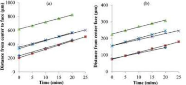
The mechanism of crystal growth of a specific crystal face can be assessed by fitting of measured growth rate data as a function of supersaturation to the models described. Figure 15 shows an example of this assessment for Ibuprofen crystals growing from different solvents.
Low spiral growth
Morphology Ibuprofen grown in 95% ethanol/5% water
(100)
(002)
(011)
High 2D nucleation
Fig. 14 Example of normal
distances from the center of the crystals to the {011} and {001} faces as a function of time. Each line represents the growth rate of an individual crystal over time: (a)
the {011} face in ethanol at =
0.66 and (b) the {001} face in
ethanol at = 0.66 (Reproduced by
[image:14.595.72.372.504.642.2]Fig. 15 Growth rate versus relative supersaturation of ibuprofen crystals growing from ethanol (blue), ethyl
acetate (red), acetonitrile (green) and toluene (purple) together with fitted B&S (solid lines) and BCF (dotted lines) mechanism models for the (011) (left) and (001) (right) faces and for both 0.5 ml (top) and 15 ml (bottom) scale sizes (Reproduced by consent of CrystEngComm from [22])
Crystallisation Process Engineering
This section will provide a practical example of crystallisation process design which includes:
Hydrodynamics and mixing in a crystalliser using computational fluid dynamics (CFD) methods,
Methodology of multi-zonal models based on the detail CFD simulation results of mixing and
hydrodynamics in crystallisers,
Morphological population balance (MPB) modelling approach for capturing crystal size and
shape distributions and their evolution during crystallisation processes,
Process scale-up studies linking to crystallisers’ size scales/configurations, operating conditions
such as agitation speed, and the internals (impeller types/materials …).
Hydrodynamics of a Batch Crystallisation Process
Hydrodynamics in a crystalliser can be very complex because the configuration of a crystalliser may be composed of moving components (such as impellers for better mixing), stagnant zones (such as the use of baffles) and the different locations of components input and product output, hence leading to non-homogeneous distributions of flow pattern, temperature, concentration, particles, etc. in the crystalliser (see for example [23-28]).
To accurately characterise the hydrodynamics in a crystalliser, both experimental measurements and numerical simulations can be used. With the advances in computational fluid dynamics (CFD) and powerful high performance supercomputers, CFD modelling methods have been widely used to characterise and capture the important flow and mixing features in a crystalliser. Such simulations can be validated with the help of experimental measurements (such as Laser Doppler Anemometry, LDA, which measures fluid velocity properties throughout a vessel as a function of agitation conditions and
[image:15.595.77.396.76.343.2]to viscous forces and consequently quantifying the relative importance of these two types of forces for given flow conditions, in a crystalliser, is one of the most important parameters to affect the mixing and flow profiles. The Re is used to characterise different flow regimes such as laminar, transition and turbulent flow according to the Re values. Generally speaking, higher Re will produce better mixing. For batch crystallisation processes, higher Re usually is generated by higher impeller speed, hence requiring higher power input and also leading to high possibility of crystal breakage. The Re can also be used to investigate the scale-up of crystallisation processes.
To simulate a crystallisation process, a multi-phase and multi-component system is required to be solved using multi-phase CFD for velocity, temperature, concentration distributions, coupled with population balance (PB) modelling for crystal size/shape distributions. The coupling can be at different levels. Traditionally, for a batch crystalliser with an impeller, a well-mixed condition is assumed, therefore a PB model can be applied to obtain the crystal size/shape distributions. However, this can cause big errors in the PB simulation as the actual conditions in a crystalliser are not homogeneous. The high level of coupling is to fully couple CFD with PB through each CFD mesh cell, i.e. treating each mesh cell as a well-mixed small reactor and applying PB to obtain size/shape distribution in this cell with the dynamic exchange of flow features information with its neighbouring cells. The fully coupling method will significantly increase the required computational time because the total mesh cells for the CFD simulation of a crystalliser can be millions in order to capture the flow/mixing features, hence the same number (millions) of PB equations needs to be solved for each time step over the crystallisation period.
Turbulence exists in almost all flows of practical engineering interests including crystallisation processes, and is inherently three-dimensional and time dependent. Due to its extreme complexity, turbulence has been recognised as the major unsolved problem of classic physics [29]. To address this issue, various turbulence models have been developed including zero-/one-equation, two-equation (k -
, k – and the variations), and Reynolds-stress models, etc. The most commonly used k - model
can be employed to represent the Reynolds-stress terms with the two equations being derived from the Navier-Stokes equation with some closure assumptions to allow simplification of the Reynolds-stress terms [29, 30].
The continuity, momentum and enthalpy conservation equations based on time-averaged quantities, together with turbulence models, are derived from Reynolds averaging of the corresponding instantaneous equations and numerically solved to obtain hydrodynamic and heat transfer profiles in crystallisers. The mixing behaviours in the crystallisers can be simulated by introducing an inert tracer into the reactors. The solution of the Reynolds-averaged species transport equations produces the spatial and temporal distributions of the tracer concentrations. For phase flow, two-fluid / multi-fluid method can be used to treat each phase as an inter-penetrated multi-fluid. Each phase will have the corresponding conservation equations with a weighing factor to be its mass fraction. For further details, please refer to literature such as [31-34] and textbooks.
Fig. 16 (a) A baffled batch crystalliser with 3-blade retreat curve impeller; (b) top-view of the reactor; (c) the
impeller. (Reproduced by consent of Ind. Eng. Chem. Res. from [35])
With the proper mesh cells, initial and boundary conditions and solution schemes, the CFD simulation of the crystalliser with water and 100 rpm impeller speed was validated by the measured velocity using LDA in a crystalliser with the same configurations (Fig. 17).
Fig. 17 Flow patterns at various vertical planes: (Top) LDA measurements; (Bottom) CFD simulations.
(Reproduced by consent of Ind. Eng. Chem. Res. from [35])
Plane at 15º Normalised radial position
N o rm al is ed ax ia l p o si ti o n
0 0.1 0.2 0.3 0.4 0.5 0 0.1 0.2 0.3 0.4 0.5 0.6 0.5 0.45 0.4 0.35 0.3 0.25 0.2 0.15 0.1 0.05 0 LDA Radial and axial velocity resultant
Tangential velocity Tip speed
Normalised radial position
N o rm al is ed ax ia l p o si ti o n
0 0.1 0.2 0.3 0.4 0.5 0 0.1 0.2 0.3 0.4 0.5 0.6 0.5 0.45 0.4 0.35 0.3 0.25 0.2 0.15 0.1 0.05 0 CFD Radial and axial velocity resultant
Tangential velocity Tip speed
Normalised radial position
N o rm al is ed ax ia l p o si ti o n
0 0.1 0.2 0.3 0.4 0.5 0 0.1 0.2 0.3 0.4 0.5 0.6 0.5 0.45 0.4 0.35 0.3 0.25 0.2 0.15 0.1 0.05 0 LDA Radial and axial velocity resultant
Tangential velocity Tip speed
Normalised radial position
N o rm al is ed ax ia l p o si ti o n
0 0.1 0.2 0.3 0.4 0.5 0 0.1 0.2 0.3 0.4 0.5 0.6 0.5 0.45 0.4 0.35 0.3 0.25 0.2 0.15 0.1 0.05 0 LDA Radial and axial velocity resultant
Tangential velocity Tip speed
Normalised radial position
N o rm al is ed ax ia l p o si ti o n
0 0.1 0.2 0.3 0.4 0.5 0 0.1 0.2 0.3 0.4 0.5 0.6 0.5 0.45 0.4 0.35 0.3 0.25 0.2 0.15 0.1 0.05 0 LDA Radial and axial velocity resultant
Tangential velocity Tip speed
Normalised radial position
N o rm al is ed ax ia l p o si ti o n
0 0.1 0.2 0.3 0.4 0.5 0 0.1 0.2 0.3 0.4 0.5 0.6 0.5 0.45 0.4 0.35 0.3 0.25 0.2 0.15 0.1 0.05 0 CFD Radial and axial velocity resultant
Tangential velocity Tip speed
Normalised radial position
N o rm al is ed ax ia l p o si ti o n
0 0.1 0.2 0.3 0.4 0.5 0 0.1 0.2 0.3 0.4 0.5 0.6 0.5 0.45 0.4 0.35 0.3 0.25 0.2 0.15 0.1 0.05 0 CFD Radial and axial velocity resultant
Tangential velocity Tip speed
Normalised radial position
N o rm al is ed ax ia l p o si ti o n
0 0.1 0.2 0.3 0.4 0.5 0 0.1 0.2 0.3 0.4 0.5 0.6 0.5 0.45 0.4 0.35 0.3 0.25 0.2 0.15 0.1 0.05 0 CFD Radial and axial velocity resultant
Tangential velocity Tip speed
Plane at 60º Plane at 120º Plane at 180º
Impeller (a)
(b)
[image:17.595.131.422.78.313.2] [image:17.595.74.522.412.721.2]Zonal Models for Crystallisers
The compromised method is to use multi-zonal model or Villermaux’s segregated feed model [36] by
which CFD simulations are performed first, and then different zones in the crystalliser are identified according to the flow/mixing features. These zones will be treated as well-mixed reactors to couple with PB modelling. This will dramatically reduce the number of PB equations to be solved, hence saving computational time. This method is particularly useful when involving large scale industrial crystallisers and investigating process scale-up.
The flow and turbulence characteristics obtained from the CFD simulation can be used to identify different mixing regions. As shown in Fig. 18, for a zonal coupling method, the crystalliser can be divided into four zones such as impeller zone (1), bottom zone (2), top zone (3) and wall zone (4).
Fig. 18 (a) Velocity vectors; (b) eddy viscosity contour. (Reproduced with permission from [37])
A tracer was introduced into the crystalliser to simulate the turbulent mixing via solving a species transport concentration equation to obtain the tracer distributions over time [33] as shown in Fig. 19.
(a) (b)
(1)
(2) (3)
[image:18.595.72.327.244.505.2]Fig. 19 Tracer concentration distributions in the vertical planes at 0 (tracer injection plane) and 180 angular
positions, which reveal the overall mixing process in the tank. (Reproduced by consent of Chem. Eng. Process. from [33])
The Segregated Feed Model (SFM) [32, 36] is a compartmental mixing model. The combination of SFM with CFD and population balance can simulate the effect of various operating conditions and reactor configurations on the nucleation rate and crystal size distribution.
Villermaux [36] proposed the SFM model based on physically meaningful mixing parameters involving:
diffusive micro-mixing time;
convective meso-mixing time.
The SFM is particularly suitable for modelling mixing effects as it combines advantages of both
compartmental model;
physical model.
SFM divides the reactor into three zones:
two feed zones f1 and f2;
bulk b.
The feed zones exchange mass with each other and also with the bulk zone. The process depicted by
flow rates u1,2, u1,3 and u2,3, respectively is shown in Fig. 20(a) [32]. The time constants characteristic
can be used to identify the micro-mixing and meso-mixing [38, 39]:
(28)
where is the specific power input; Am is a constant from literature [38, 39]; ds is the diameter of a
[image:19.595.77.522.70.291.2]Qf1 Qf2
u1,2
u1,3 u2,3
Qb
reaction
plume f1
reaction
plume f2
bulk b
Hydrodynamic model (CFD)
Population balance
Mixing model (Segregated Feed
Model SFM)
Laboratory-scale experiments
Large-scale reactor
(a) (b)
Fig. 20 (a) Schematic of segregated feed model, (b) scale-up methodology with SFM approach (Reproduced by
consent of Ind. Eng. Chem. Res. from [32])
As shown in Fig. 20(b) [32], the scale-up methodology using SFM involves the following steps:
• Carry out laboratory scale measurements;
• Model hydrodynamics via computational fluid dynamics (CFD);
• Use population balance model for particle properties (number/size distribution);
• Link two models via segmented feed model (SFM);
• Predict precipitation performance as a function of scale size.
Morphological Population Balance Models
A population balance (PB) model generally accounts for the convective processes that involve both the motion of particles in a system through their defined domains and their birth-and-death processes that
can both terminate existing particles and produce new particles. The generic mathematical formulation
for multidimensional PB modeling can be given by the following equation:
(29)
where N is the number of internal variables for a crystal, x is the internal variable vector with n
components, which can be parameters related to crystal size, shape, and other properties; y is the
external variable vector such as spatial coordinates (y1, y2, y3); n is the number population density
function of crystals in the internal variable range (xi, xi + dxi, i = 1, N) and in the differential volume of
dy1dy2dy3; is the gradient operator for the y coordinates. On the left-hand side, the 1st term is the
accumulation term of n; the 2nd term denotes the convection of n in the y space with v being the
velocity vector; the 3rd term is the convection of n due to particle growth in the x space with G
i being
the growth rate; the 4th term is the net change of n during residence time,
r, due to the inlet and outlet
flows of continuous crystallization processes with n0 being the initial number population density
[image:20.595.80.506.70.342.2]birth and death terms of n for agglomeration and breakage, and the third term B0(x, y, t) for nucleation.
Indices a, d, and 0 relate to agglomeration, breakage and nucleation.
In a well-mixed crystalliser, Eq. (32) becomes the PB equation proposed by Randolph and Larson [40]:
(30)
Although population balance (PB) modeling for crystallization processes is for all crystals in a crystallizer, crystal shape was often ignored with an over-simplified crystal-size definition, i.e., the volume equivalent diameter of spheres or simplified as length and width for some needle-like crystals
[41]. A morphological population balance (MPB) model is able to incorporate any complicated crystal
structures/shapes into PB modeling, therefore, can simulate the size-related dimensional evolution of crystals for each identified independent crystal face (for further details, see [42, 43]). From the predicted growth of different faces at different times during crystallization process, many important crystal properties, such as shape and growth rate can be evaluated and used for real-time monitoring, control and manipulation of crystal morphology.
The MPB models define the multiple dimensions of PB number density as the distances of each face to its geometric centre, hence being able to fully re-construct the shape of any one crystal at any time and also taking into account different growth kinetics for different crystal faces. Taking a potash alum
crystal as an example, a 3D MPB model, the corresponding three parameters, x1, x2, x3, shown in Fig.
21, can be formed to model its morphological changes in a well-mixed batch crystallizer with
breakage, agglomeration and nucleation being ignored. The MPB equation of Eq. (30) can, thus, be
written as follows:
(31)
The crystal shape evolution as shown in Fig. 22 demonstrates that the {100} and {110} faces will eventually disappear with the crystal expected to exhibit pure octahedral diamond-like morphology at steady state under the current simulation conditions, which has been observed in literature.
x3 x2
[image:21.595.285.471.319.494.2]x1
Fig. 21 Morphology of potash alum crystal
and schematic diagram of the three size characteristic parameters (x1, x2, x3) to be used
Fig. 22 Crystal shape evolution during the crystallisation process of potash alum. (Reproduced by consent of
AIChE J. from [42])
For the crystallisation of potash alum crystals, the growth rate dispersion (GRD) may play a role
particularly on the faster growing {100} faces, especially for larger crystals (~cm). Growth sector
boundaries predicted from the MPB simulations with and without GRD and measured by experiment are plotted in Fig. 23. The faces {100} and {110} clearly tend to disappear completely (Fig. 23) if GRD effect is not included in the simulations. However, when the GRD is included, all three habit faces show continuous growth at variable speeds, which is close to that found in experiments.
Fig. 23 Growth sector boundaries of a typical potash alum crystal (a) predicted by the MPB model with
(coloured in red) and without (coloured in black) including GRD effect (Reproduced by consent of AIChE J. from [43]) and (b) measured by experiments (Reproduced by consent of Chem. Eng. Technol. from [44])
By comparing the predicted growth sector boundaries with GRD effect (Fig. 23(a)) with the experimentally measured boundaries (Fig. 23(b)), the results are in qualitative agreement.
Crystallisation Process Scale-up
The PB modelling method is a scalable technique which can be directly applied to large and small scale systems. However, as shown in Eq. (33), the crystal size/shape distributions are affected by the mechanisms/kinetics of nucleation, growth, agglomeration, breakage, etc. which are directly related to the flow pattern and mixing, mass and heat transfer in a reactor. The two-way interactions between CFD and MPB modelling can be achieved via either zonal coupling or mesh-to-mesh fully CFD-MPB coupling. The coupled CFD-MPB modelling method will have great potential for the scale-up of crystallisation processes and further research is needed. As we understand, the physical phenomena in a crystalliser play very important roles in the process scale-up, which include mass transfer, heat transfer, physical properties of solute and solvent, etc. The process scale-up can be performed by
700 Time (s)
500 900 1100 1300 1500
(a)
[image:22.595.75.487.71.212.2] [image:22.595.89.513.354.531.2]simple geometrical similarity which may not achieve the corresponding mixing, particle quality, if flow characteristics in the two reactors are not similar. For dynamic and kinematic similarities, the ratio of forces in a process, and the velocity at similar locations (such as impeller tip) can be kept
constant during scale-up. Furthermore, the crystallisers’ internals such as impeller types and materials
can also affect the performance of the crystallisation processes during scale-up.
Liang et al. [28, 45] investigated the effects of reactor internals [28] and reactant mixing [45] on the measured MSZW associated with the batch crystallisation of L-glutamic acid from supersaturated aqueous solutions. The cooling crystallisation experiments were carried out at three reactor scales (450 mL, 2 L and 20 L) agitated at various stirring speeds using an industry-standard retreat curve impeller with a single beaver-tail baffle. Nucleation kinetic parameters at 450 mL were evaluated using a method proposed by Ny´vlt et al. [5]. It was found that increased mixing generally is capable of enhancing the nucleation rate, but with a further increase of the stirrer speed beyond a critical value, aeration was observed and this may contribute to the reduced nucleation. The measured MSZWs are mostly found to decrease with increasing stirring speed, with enhanced nucleation also being observed as the reactor scale increased (Fig. 24); albeit hindered nucleation was found at higher stirrer speeds in the 450 mL reactor experiments (Fig. 25).
From Fig. 24, a linear relationship (Eq. 32) between MSZW and the stirrer speed was obtained by least-squares linear regression analysis.
[image:23.595.259.501.299.686.2]tmax = -0.0464 Ns + 35.109 (32)
Fig. 24 MSZW as a function of the
stirrer speed in 450-mL, 2-L, and 20-L reactors at a cooling rate of 0.2 °C/min (Reproduced by consent of Ind. Eng. Chem. Res. from [45])
Fig. 25 Calculated nucleation rate as a
Where tmax is the maximum possible supercooling of the system and Ns is the stirrer speed. This
revealed that the stirrer speed is a significant parameter of the current system. However, for a general model application it needs to correlate the nucleation process to the reactor hydrodynamics as characterised by the Reynolds number. Through combining the influence of reactor hydrodynamics and scale on mass transfer during the crystallization process, a general correlation was postulated, including the method for nucleation kinetics from Ny´vlt et al. [5] and the definition of the maximum
possible supersaturation cmax as a function of tmax. It was fitted with experimental data (as shown in
Fig. 26) using multiple nonlinear regression analysis to yield Eq. (33):
(33)
where tsat is the saturated temperature, Re is the Reynolds number, T0 is the diameter of the laboratory
reactor and T/T0 is the scale-up ratio. It is suggested that the correlation provides a good estimate of
MSZW in an agitated vessel for the system examined. It is also concluded that mixing affects the surface-induced heterogeneous nucleation process by thinning the boundary layer at the stirrer blade surface.
Liang et al. [28] reported that primary nucleation can be affected by stirrer material. In the study, batch cooling crystallizations of L-glutamic acid aqueous solutions were carried out in a 450 mL reactor using stirrers with identical geometry but made from different materials: stainless steel and Perspex. It was found that there existed a high degree of crystal encrustment on the surface of the stirrers and impeller shaft with much denser crystal attachments on the blades of the stainless steel stirrer than on the Perspex one. This strongly indicated that the nucleation process initially started on the surface of the stirrer rather than in the preferentially cooled regions adjacent to the reactor wall as would be more
conventionally accepted. By using measured MSZW for nucleation kinetics analysis, both stirrers
[image:24.595.197.486.306.490.2]showed similar MSZW profiles as a function of stirring rate, though nucleation was found to be much easier with the stainless steel stirrer. Nucleation order obtained from the experiments performed with the stainless steel stirrer were found to be greater than those with the Perspex stirrer, i.e., consistent with a much lower energy barrier for nucleation in the case of the stainless steel stirrer. However, the data also show that the nucleation rate constant for experiments carried out using the Perspex stirrer were much higher than those when using the stainless steel impeller for the same agitation rate. Figure 27 shows the measured advancing contact angle and free energy ratio of L-glutamic acid aqueous solutions on both Perspex and stainless steel flat plates.
Fig. 26 Fitting experimental data with
The encrustment observations together with experimental measurements (Fig. 27) of contact angle for different stirrer materials, from which the free energy ratio was calculated, confirm that the energy needed to form critical nuclei on the stainless steel surface would be much lower than on Perspex. Surface roughness is also believed to play an important role. Overall, these observations are consistent with the stirrer surface providing preferred nucleation sites in L-glutamic acid crystallization with both the stirrer material and its surface roughness being important factors dictating the nature of the primary nucleation process. It also appears that nucleation occurs first on the surface of the stirrer, where the strongest turbulent kinetic energy is present. Hence, it is reasonable to conclude that these newly formed nuclei grow continuously to critical nuclei as freshly supersaturated solution is transported to the region due to better micromixing compared to that in the rest of the bulk. These stable nuclei may then be washed away by the strong fluid shear force and quickly dispersed into other parts of the bulk in the crystallizer and then the overall nucleation event is triggered. Therefore, this study [28] reveals a heterogeneous nucleation mechanism involving a surface-induced process on the stirrer surface with the surface properties and its material of construction playing an important role by the overall crystallization process.
Li et al. [46] used CFD simulations to investigate the scale up effects for three geometrically similar laboratory scale vessels of 0.5, 2 and 20 L with retreat curve impellers and cylindrical baffles, which mimic reactors widely used in the pharmaceutical and fine chemical industries. CFD results have then been validated using LDA measurements and empirical power consumption literature data. The comparisons of power number, discharge flow number, secondary circulation flow number and pumping efficiency at three different scales suggest that the scale up with the selected laboratory vessels has little effect on the macro mixing performance for optimisation of the configuration and operating conditions of an industrial scale reactor. Further details about the experimental and modelling investigations of process scale-up can be found in the literature, such as [28, 32, 45-49].
Concluding Remarks
[image:25.595.245.515.83.277.2]The objective of this crystallisation route map is to lay the foundation for the crystallisation processes, which covers the solubility and solution ideality for crystallisation processes, the supersaturation, MSZW and its impact on product form through the use of supersaturation to control nucleation and growth processes, the nucleation and its kinetic characterisation, the crystal growth and its measurement together with characterising the growth mechanisms, and the hydrodynamics of crystallisation processes, population balance modelling, and crystallisation scale-up.
Fig. 27 Dependence of advancing
contact angle and free energy ratio on surface types and concentration of aqueous L-glutamic acid
List of Symbols
(hkl) – Miller plane - 2D surface cut through lattice
– dimensionless molecular latent heat of crystallisation
and – free parameters in PN model
Am– a constant from literature [35, 36]
and – system related constants
b – bulk compartment in SFM
– dimensionless thermodynamic parameter
Ba(x, y, t) and Da(x, y, t) – birth and death terms of n for agglomeration
Bd(x, y, t) and Dd(x, y, t) – birth and death terms of n for breakage
B0(x, y, t) – nucleation term
– solution concentration
– equilibrium concentration
C – maximum supersaturated concentration
C – concentration of nuclei at the IN point
– characteristic dimension
– dimensionality of crystal growth
ds – diameter of a stirrer
f1, f2– feed compartments in SFM
gi– face growth rate in i direction
Gi– Growth rate
J – nucleation rate
– empirical parameter of nucleation rate
– nucleus shape factor
– crystal shape factor
– growth rate constant
– nucleation rate constant
– order of nucleation
n – number population density function of crystals
n0– initial number population density function of crystals
and – growth exponents
N – number of internal variables for a crystal
Ns– stirrer speed
– number of crystals at detection point
– cooling rate
– free parameters in PN model
Q – flow rate of a stream
– nucleus radius
R – gas constant
– rate of growth of a crystal face
Re – Reynolds number
– nucleus critical radius
– supersaturation
– temperature
– scale up ratio
– diameter of the laboratory reactor
– crystallisation temperature
– dissolution temperature
– solution equilibrium temperature
– fusion temperature of pure solute
t – time
t – saturation temperature
u1,2, u1,3 & u2,3– flow rates
V – velocity
– volume occupied by a solute molecule in the crystal
v – velocity vector
– mole fraction
– normal distances
x – internal variable vector with N components
y – external variable vector such as spatial coordinates (y1, y2, y3)
– surface entropy factor
– relative volume of crystals at detection point
– activity coefficient
– interfacial tension and/or surface energy
– density
– maximum concentration difference
– entropy of dissolution
– enthalpy of fusion of pure solute
– enthalpy of dissolution
- entropy of fusion of pure solute
– critical undercooling for crystallisation
t – metastable zone width
– specific power input
– anisotropy factor
– Boltzmann constant
– molecular latent heat of crystallisation
– fluid dynamic viscosity
– relative critical undercooling at the IN point
– relative critical undercooling
– relative supersaturation
– induction time
r– residence time
– molecular volume
– gradient operator for the y coordinates
References
1. Prausnitz JM (1969) Molecular thermodynamics of fluid-phase equilibria Prentice-Hall Inc.,
Englewood Cliffs N. J.
2. Dickerson RE (1969) Molecular thermodynamics W. A. Benjamin, New York
3. Davey RJ, Mullin JW, Whiting MJL (1982) Habit modification of succinic acid crystals grown from different solvents Journal of Crystal Growth 58:304-3l2
4. Mullin JW (2001) Crystallization, 4th edn Butterworth-Heinemann, Oxford
5. Nyvlt J (1968) Kinetics of nucleation in solutions Journal of Crystal Growth 4:377-383.
6. Nyvlt J, Rychly R, Gottfried J, Wurzelova J (1970) Metastable Zone Width of some aqueous
solutions Journal of Crystal Growth 6:151-162
7. van Gelder RNMR, Roberts KJ, Chambers J, Instone T (1996) Nucleation of single and mixed straight chain surfactants from dilute aqueous solutions. Journal of Crystal Growth 166:189-194
8. Kashchiev D, Borissova A, Hammond RB, Roberts KJ (2010) Dependence of the critical
undercooling for crystallization on the cooling rate. Journal of Physical Chemistry B 114:5441-5446
9. Kashchiev D, Borissova A, Hammond RB, Roberts KJ (2010) Effect of cooling rate on the
10. Camacho D, Borissova A, Hammond R, Kashchiev D, Roberts K, Lewtas K, More I (2014) Nucleation mechanism and kinetics from the analysis of polythermal crystallisation data: methyl stearate from kerosene solutions. CrystEngComm 16:974-991
11. Kashchiev D (2000) Nucleation: basic theory with applications Butterworth-Heinemann, Oxford. 12. Toroz D, Rosbottom I, Turner T, Camacho DM, Hammond RB, Roberts KJ (2015) Towards an
understanding of the nucleation of alpha-para amino benzoic acid from ethanolic solutions: a multi-scale approach. Faraday Discussions 179:79-114
13. Sangwal K (2007) Additives and crystallization processes : from fundamentals to applications Wiley, Chichester
14. Roberts KJ, Sherwood JN, Stewart A (1990) The nucleation of n-eicosane crystals from solutions in n-dodecane in the presence of homologous impurities. Journal of Crystal Growth 102:419-426. 15. Boistelle R, Astier JP (1988) Crystallization mechanisms in solution. Journal of Crystal Growth
90:14-30
16. Frank FC (1949) The influence of dislocations on crystal growth. Faraday Discussions 5:48-54 17. Elwell D, Scheel HJ (1975) Crystal growth from high temperature solutions. Crystal Research &
Technology 11:K28-K29
18. Weeks JD, Gilmer GH (1979) Dynamics of Crystal Growth. Advances in Chemical Physics 40:157-227
19. Jackson KA (1958) Mechanisms of Growth. In: Metals ASf (ed) Liquid Metals and Solidification, Cleveland
20. Jetten LAMJ, H.J. H, Bennema P, van der Eerden JP (1984) On the observation of the roughening transition of organic crystals, growing from solution. Journal of Crystal Growth 68:503-516 21. Human HJ, Van der Eerden JP, Jetten LAMJ, Odekerken JGM (1981) On the roughening
transition of biphenyl: transition of faceted to non-faceted growth of biphenyl for growth from different organic solvents and the melt. Journal of Crystal Growth 51:589-600
22. Nguyen TTH, Hammond RB, Roberts KJ, Marziano I, Nichols G (2014) Precision measurement of the growth rate and mechanism of Ibuprofen {001} and {011} as a function of crystallisation environment. CrystEngComm 16:4568-4586
23. Gron H, Borissova A, Roberts KJ (2003) In-process ATR-FTIR spectroscopy for closed-loop supersaturation control of a batch crystallizer producing monosodium glutamate crystals of defined size. Industrial & Engineering Chemistry Research 42:198-206
24. Gron H, Mougin P, Thomas A, White G, Wilkinson D, Hammond RB, Lai XJ, Roberts KJ (2003) Dynamic in-process examination of particle size and crystallographic form under defined conditions of reactant supersaturation as associated with the batch crystallization of monosodium glutamate from aqueous solution. Industrial & Engineering Chemistry Research 42:4888-4898 25. Haque JN, Mahmud T, Roberts KJ, Rhodes D (2006) Modeling turbulent flows with free-surface
in unbaffled agitated vessels. Industrial & Engineering Chemistry Research 45:2881-2891 26. Haque JN, Mahmud T, Roberts KJ, Liang JK, White G, Wilkinson D, Rhodes D (2011)
Free-Surface Turbulent Flow Induced by a Rushton Turbine in an Unbaffled Dish-Bottom Stirred Tank Reactor: Ldv Measurements and Cfd Simulations. Canadian Journal of Chemical Engineering 89:745-753
27. Mahmud T, Haque JN, Roberts KJ, Rhodes D, Wilkinson D (2009) Measurements and modelling of free-surface turbulent flows induced by a magnetic stirrer in an unbaffled stirred tank reactor. Chemical Engineering Science 64:4197-4209
28. Liang K, White G, Wilkinson D, Ford LJ, Roberts KJ, Wood WML (2004) An examination into the effect of stirrer material and agitation rate on the nucleation of L-glutamic acid batch crystallised from slow-cooled supersaturated solutions. Crystal Growth & Design 4:1039-1044. 29. Wilcox DC (2006) Turbulence Modeling for CFD DCW Industries, Inc.
30. Launder BE, Reece GJ, Rodi W (1975) Peogress in the development of a Reynolds-stress turbulence closure. Journal of Fluid Mechanics 68:537-566
31. Rane CV, Ganguli AA, Kalekudithi E, Patil RN, Joshi JB, Ramkrishna D (2014) CFD simulation and comparison of industrial crystallizers. Canadian Journal of Chemical Engineering 92:2138-2156.
33. Javed KH, Mahmud T, Zhu JM (2006) Numerical simulation of turbulent batch mixing in a vessel agitated by a Rushton turbine. Chemical Engineering Processing 45:99-112
34. Ma CY, Liu JJ, Zhang Y, Wang XZ (2015) Simulation for scale-up of a confined jet mixer for continuous hydrothermal flow synthesis of nanomaterials. J Supercrit Fluids 98:211-221
35. Li MZ, White G, Wilkinson D, Roberts KJ (2004) LDA measurements and CFD modeling of a stirred vessel with a retreat curve impeller. Industrial & Engineering Chemistry Research 43:6534-6547
36. Villermaux J (1989) A simple model for partial segregation in a semibatch reactorAIChE Annual Meeting, San Francisco CA, pp. paper 114a
37 Jones RM, Rouge B, Harvey III AD, Acharya S (2001) Two-equation turbulence modeling for impeller stirred tanks. Trans. ASME, Journal of fluids engineering 123:640-648
38. Batdyga J, Bourne JR, Hearn SJ (1997) Interaction between chemical reactions and mixing on various scales. Chemical Engineering Science 52:457-466
39. Batdyga J, Podgorska W, Pohorecki R (1995) Mixing-precipitation model with application to double feed semibatch precipitation. Chemical Engineering Science 50:1281-1300
40. Randolph AD, Larson MA (1962) Transient and steady state size distributions in continuous mixed suspension crystallisers. AIChE J 8:639-645
41. Ma CY, Wang XZ, Roberts KJ (2007) Multi-dimensional population balance modeling of the growth of rod-like L-glutamic acid crystals using growth rates estimated from in-process imaging. Advanced Powder Technology 18:707-723
42. Ma CY, Wang XZ, Roberts KJ (2008) Morphological population balance for modeling crystal growth in face directions. AIChE J 54:209-222
43. Ma CY, Wang XZ (2008) Crystal growth rate dispersion modelling using morphological popultion balance. AIChE J 54:2321-2334
44. Lacmann R, Herden A, Mayer C (1999) Kinetics of nucleation and crystal growth. Chemical Engineering & Technology 22:279-289
45. Liang KP, White G, Wilkinson D, Ford LJ, Roberts KJ, Wood WML (2004) Examination of the process scale dependence of L-glutamic acid batch crystallized from supersaturated aqueous solutions in relation to reactor hydrodynamics. Industrial & Engineering Chemistry Research 43:1227-1234
46. Li MZ, White G, Wilkinson D, Roberts KJ (2005) Scale up study of retreat curve impeller stirred tanks using LDA measurements and CFD simulation. Chemical Engineering Journal 108:81-90 47. Khan S, Ma CY, Mahmud T, Penchev RLY, Roberts KJ, Morris J, Ozkan L, White G, Grieve B,
Hall A, Buser P, Gibson N, Keller P, Shuttleworth P, Price CJ (2011) In-process monitoring and control of supersaturation in seeded batch cooling crystallisation of L-glutamic acid: from laboratory to industrial pilot plant. Organic Process Research & Development 15:540-555
48. Li R, Penchev R, Ramachandran V, Roberts KJ, Wang XZ, Tweedie R, Prior A, Gerritsen J, Hugen F (2008) Particle shape characterisation via image analysis: From laboratory studies to in-process measurements using an in-Situ Particle Viewer (ISPV) system. Organic Process Research & Development 12:837-849
![Fig. 2 Ideal and experimental solubility for succinic acid in water and isopropanol [3]](https://thumb-us.123doks.com/thumbv2/123dok_us/7736539.164032/4.595.256.499.586.774/fig-ideal-experimental-solubility-succinic-acid-water-isopropanol.webp)
![Fig. 5 Transmittance versus temperature for a turbidity probe in a crystallising solution (Reproduced by consent of J Crystal Growth from [7])](https://thumb-us.123doks.com/thumbv2/123dok_us/7736539.164032/8.595.72.484.458.672/transmittance-temperature-turbidity-crystallising-solution-reproduced-consent-crystal.webp)
![Fig. 15 Growth rate versus relative supersaturation of ibuprofen crystals growing from ethanol (blue), ethyl acetate (red), acetonitrile (green) and toluene (purple) together with fitted B&S (solid lines) and BCF (dotted lines) mechanism models for the (011) (left) and (001) (right) faces and for both 0.5 ml (top) and 15 ml (bottom) scale sizes (Reproduced by consent of CrystEngComm from [22])](https://thumb-us.123doks.com/thumbv2/123dok_us/7736539.164032/15.595.77.396.76.343/relative-supersaturation-ibuprofen-crystals-acetonitrile-mechanism-reproduced-crystengcomm.webp)
