Long-distance continuous-variable quantum key distribution with quantum scissors

with quantum scissors

.

White Rose Research Online URL for this paper:

http://eprints.whiterose.ac.uk/142978/

Article:

Ghalaii, Masoud, Ottaviani, Carlo orcid.org/0000-0002-0032-3999, Kumar, Rupesh et al. (2

more authors) (2018) Long-distance continuous-variable quantum key distribution with

quantum scissors. arXiv.

[email protected] https://eprints.whiterose.ac.uk/

Reuse

Items deposited in White Rose Research Online are protected by copyright, with all rights reserved unless indicated otherwise. They may be downloaded and/or printed for private study, or other acts as permitted by national copyright laws. The publisher or other rights holders may allow further reproduction and re-use of the full text version. This is indicated by the licence information on the White Rose Research Online record for the item.

Takedown

If you consider content in White Rose Research Online to be in breach of UK law, please notify us by

Masoud Ghalaii,1Carlo Ottaviani,2 Rupesh Kumar,3 Stefano Pirandola,2 and Mohsen Razavi1 1

School of Electronic and Electrical Engineering, University of Leeds, Leeds LS2 9JT, United Kingdom

2_{Computer Science and York Centre for Quantum Technologies, University of York, York YO10 5GH, United Kingdom} 3

Department of Physics, University of York, York YO10 5DD, United Kingdom

(Dated: August 7, 2018)

The use of quantum scissors, as candidates for non-deterministic amplifiers, in continuous-variable quantum key distribution systems is investigated. Such devices rely on single-photon sources for their operation and as such, they do not necessarily preserve the Guassianity of the channel. Using exact analytical modeling for system components, we bound the secret key generation rate for the system that uses quantum scissors. We find that for non-zero values of excess noise such a system can reach longer distances than the system with no amplification. The prospect of using quantum scissors in continuous-variable quantum repeaters is therefore emboldened.

PACS numbers: 03.67.Dd, 03.67.Hk

I. INTRODUCTION

Quantum key distribution (QKD) [1,2] addresses the prob-lem of sharing secret keys between two users. Such keys can then be used for secure communications. While origi-nal QKD protocols [1–4] rely on encoding data in discrete quantum states, such as the polarization of single photons, one can also exploit continuous-variable QKD (CV QKD) proto-cols, in which data is encoded on the quadratures of the light [5–8]. In particular, the recent progress in CV QKD systems has placed them in a competitive position with their conven-tional discrete-variable counterparts [9, 10]. For instance, contrary to discrete-variable QKD protocols, which require single-photon detectors, CV QKD uses coherent measurement schemes, such as homodyne and/or heterodyne detection, to measure light quadratures, without relying on photon count-ing devices [11–13]. Moreover, CV QKD protocols can be the better choice over short distances [10]. Once it comes to long distances, however, CV QKD has its own challenges to com-pete with discrete-variable QKD [14]. This paper examines how the security distance can be enhanced in CV QKD sys-tems by using realistic non-deterministic amplification [15].

One of the proposed solutions to improve the rate-versus-distance performance of CV QKD protocols is to use noiseless linear amplifiers (NLAs) [15,16]. It is known that determinis-tic amplification cannot be noise free [17]. An NLA can only then workprobabilistically. This inevitably reduces the key rate by a factor corresponding to the success rate of the NLA, which implies that, at short distances, the use of NLAs may not be beneficial. The key rate may, however, increase at long distances because of the improvement in the signal to noise ratio. That is, while the number of data points we can use for key extraction is less, the quality of the remaining points could be such high that a larger number of secret key bits can be extracted. This has been shown theoretically by treating the NLA as a probabilistic, butnoiseless, black box and assum-ing that the NLA achieves its theoretically maximum possible success rate for all possible inputs [15].

The story can be quite different when we replace the above ideal NLA with realistic systems that offer NLA-like func-tionality. For instance, one of the most basic structures for an

NLA is a quantum scissor (QS), which combines the incom-ing light with a sincom-ingle photon [18]. While under weak signal assumptions, a QS can be approximated as an NLA, more pre-cise analysis reveals that its operation is not necessarily noise-less. This is particularly important because in many CV QKD protocols the transmitted signal does not have a fixed power, and realistic NLAs often treat different input signals differ-ently. This is more or less true for other proposals that imple-ment the NLA operation [19–24].

In this paper, we provide a realistic account of what a QS can offer within a CV QKD setup. In particular, using an ex-act model for the QS setup, we analyze the secret key rate of a Gaussian modulated protocol, whose receiver unit is equipped with a QS. One of the implications of our exact modeling for the QS is the inapplicability of standard key rate calculation techniques that rely on the Gaussianity of the output states. This will make the exact calculation of the key rate cumber-some. We manage this problem by using relevant bounds for certain components of the key rate. We find that by using the QS we can exchange secret keys over longer distances. Our work also provides insights into the practicality of the recent proposals for CV quantum repeaters [25,26].

The manuscript is structured as follows. In Sec.II, we de-scribe details of the proposed system. In Sec.III, by analyz-ing input-output characteristic functions of a sanalyz-ingle QS, we calculate the exact output state and success probability of the QS NLA in Ref. [18]. We further study the non-Gaussian be-havior of the system. In Sec.IV, we present the key rate analy-sis of the CV QKD link with a single QS as part of its receiver. In Sec.V, we discuss the numerical results. Finally, Sec.VI

concludes the paper.

II. SYSTEM DESCRIPTION

In this section, we describe our proposed setup for the QS-amplified CV QKD protocol. We assume that the sender, Al-ice (A), is connected to the receiver, Bob (B), via a quan-tum channel; see Fig.1(a). The protocol runs along the same lines as proposed by Grosshans and Grangier in 2002 (GG02) [5,6,27,28]. That is, in every round, Alice transmits a

FIG. 1. (a) Schematic view of CV QKD link with an additional quantum scissor at the receiver. A beam splitter with transmittiv-ityT characterizes the quantum channel, with excess noise at the input represented byε. (b) Entanglement-based CV QKD protocol equivalent to (a). QS, Hom and Het boxes represent, respectively, a non-deterministic quantum scissor, the homodyne detection and het-erodyne detection modules.

herent state|αi, whereα=xA+ipA, to Bob, with real

pa-rametersxAandpAbeing chosen randomly according to the

following Gaussian probability density functions:

fXA(xA) =

e−

x2_A VA/2

p

πVA/2

and fPA(pA) =

e−

p2_A VA/2

p

πVA/2

, (1)

whereVAis the modulation variance in the shot-noise units.

At the receiver, however, we equip Bob with a single QS be-fore the homodyne module used in GG02. Upon a success-ful QS operation, Bob randomly chooses to measurexˆB =

ˆ

aB + ˆa†B or pˆB = (ˆaB −ˆa†B)/i, where aˆB represents the

annihilation operator for the output mode of the QS. During the sifting stage, Bob would then publicly declare his mea-surement choices as well as the rounds in which the QS has been successful. Alternatively, one can use the equivalent entanglement-based (EB) scheme of Fig.1(b), where Alice’s source is replaced with an EPR source followed by heterodyne detection. In either case, we assume that Bob can reconstruct, in an error-free way, the phase reference for the local oscilla-tor used in his homodyne detection. By using post-processing techniques, Alice and Bob extract a key from the subset of data for which the QS has been successful.

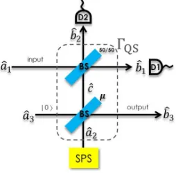
Quantum scissors are the main building blocks in the NLA proposed by Ralph and Lund [18]. At the core of a QS, there is a partial Bell-state measurement (BSM) module, with a balanced beam splitter followed by two single-photon de-tectors, in the space spanned by number states |0iand|1i. This BSM module is driven by an asymmetric entangled state

|ψi=√µ|1ic|0ib3+

√

1−µ|0ic|1ib3, generated by a single

photon that goes through a beam splitter with transmittanceµ; see Fig.2. For an input state in the|0i-|1ispace, the QS could then offer an asymmetric teleportation functionality, whenever the BSM operation is successful, i.e., when only one of D1 or D2 detector in Fig.2clicks. For instance, in the particular case of a weak coherent state input|αia1 ≈ |0ia1+α|1ia1, with

|α| ≪ 1, a single click could come from the single-photon component in the entangled state_|ψi and/or the input state. In that case, the output state, after renormalization, can be ap-proximated by|0ib3+αg|1ib3 ≈ |αgib3, for|gα| ≪1, where

g=p(1−µ)/µ represents the amplification gain of the QS.

FIG. 2. The schematic diagram of a quantum scissor. Here, we as-sume that an on-demand ideal single-photon source (SPS) is in use, and that the single-photon detectors have unity efficiencies.

Under these assumptions, the success probability for the QS operation is given byPRL

succ(α)≈µ+ (1−µ)|α|2. Note that, in the above description, the essential assumption for a QS to possibly operate as an NLA is that|α| ≪1.

There are two reservations in using the above asymptotic approach for analyzing a QS-based CV QKD system. First, note that the output state of a QS is always in the space spanned by single-photon and vacuum states. By approxi-mating the output state as a coherent state, we are introduc-ing some errors, which can affect the security of the system. More precisely, the transition from a coherent state to a single-photon state is a non-Gaussian one, whose effect must be care-fully considered in the security analysis. Secondly, in the GG02 protocol, the coherent states are chosen randomly via Gaussian distributions; hence, the input states to the QS may not necessarily satisfy the assumption|α| ≪1.

In order to resolve the above issues, in our work, we find theexactoutput state and probability of success for an arbi-trary coherent state at the input of a QS. This will be detailed in Sec.III. We then apply our findings to the key rate analysis of a QS-equipped CV QKD system. For simplicity, we as-sume that the required single-photon source (SPS) in the QS is ideal and on-demand. Single-photon detector efficiencies are also assumed to be unity. Our analysis can, nevertheless, be extended to account for the imperfections in the source and detectors.

III. QUANTUM SCISSORS: INPUT-OUTPUT

RELATIONSHIP

In this section, we first obtain an exact input-output rela-tionship for a QS driven by a coherent state. We use charac-teristic functions to model the input and output states. For a joint,M-mode, stateρˆ, where each modejis represented by an annihilation operatorˆaj, the anti-normally ordered

charac-teristic function is given by

χρ_Aˆ(ξ1, . . . , ξM) =

D_OM

j=1

ˆ

DA(ˆaj, ξj)

E

ˆ

whereh◦iρˆ ≡Tr[ˆρ◦]andDˆA(ˆa, ξ) =e−ξ ∗_ˆa

eξˆa†

is the anti-normally ordered displacement operator with ξ∗ _{being the} complex conjugate of the complex number ξ = ξr +iξi,

whereξrandξiare real numbers. The density matrixρˆand its

anti-normally ordered characteristic function are related via a Fourier-like transformation relationship as follows

ˆ ρ=

Z _d2_ξ

1

π · · ·

Z _d2_ξ

M

π χ

ˆ

ρ

A(ξ1, . . . , ξM) M

O

j=1

ˆ

DN(ˆbj, ξj),

(3)

where DˆN(ˆa, ξ) = eξaˆ †

e−ξ∗ˆa is the normally-ordered dis-placement operator andRd2ξ=R_−∞+∞dξrR_−∞+∞dξi.

In the following, we use the above formalization, to char-acterize a QS driven by an arbitrary coherent state.

A. Pre-measurement state

For the QS in Fig.2, we can use the well-known relation-ships for beam splitters to relate the three input modes of the linear circuit, represented byaˆ1,aˆ2 andˆa3, to the three out-put modes, represented byˆb1, ˆb2 andˆb3. In fact, we have

[ˆb1ˆb2ˆb3]T= ΓQS[ˆa1ˆa2ˆa3]T, where

ΓQS= √1

2

 

1 √µ −√1−µ

−1 √µ −√1−µ 0 p2(1−µ) √2µ



. (4)

The output anti-normally ordered characteristic function can then be expressed in terms of the input one by

χoutA (ξ1, ξ2, ξ3) =hDˆA(ˆb1, ξ1) ˆDA(ˆb2, ξ2) ˆDA(ˆb3, ξ3)i

=hDˆA(ˆa1, λ1) ˆDA(ˆa2, λ2) ˆDA(ˆa3, λ3)i

=χin

A(λ1, λ2, λ3), (5)

where[λ1 λ2 λ3]T = ΓTQS[ξ1 ξ2 ξ3]T with ΓTQS being the transpose of ΓQS. In above, we made use of the facts that

ˆ

DA(sˆa, ξ) = ˆDA(ˆa, sξ), where s is a real number, and hDˆA(ˆa, ξ1) ˆDA(ˆa, ξ2)i = eξ1ξ

∗

2hDˆ

A(ˆa, ξ1+ξ2)i. Note that

ΓQSis unitary, i.e.,ΓTQS= Γ−QS1. Hence, we have

P

j|ξj|2=

P

j|λj|2.

Next, for the particular input state|αiˆa1|1iaˆ2|0iˆa3 the

out-put characteristic function can be found as follows

χoutA (ξ1, ξ2, ξ3) =Tr

|αiˆa1hα| ⊗ |1iaˆ2h1| ⊗ |0iˆa3h0|

ˆ

DA(ˆa1, λ1) ˆDA(ˆa2, λ2) ˆDA(ˆa3, λ3)

=e−|λ1|2−|λ2|2−|λ3|2_eαλ¯ 1−α¯λ1₍₁

− |λ2|2), (6)

which can be re-written as the following:

χoutA (ξ1, ξ2, ξ3) =e−|ξ1|

2

−|ξ2|2−|ξ3|2_e

√

2iIm[ ¯α(ξ1−ξ2)]

×(1−µ₂|ξ1+ξ2+

s

2(1−µ) µ ξ3|

2_),

(7)

withIm[ξ]being the imaginary part of the complex numberξ. Using Eq. (3), the output state of the system is then given by

ˆ ρout =

Z _d2_ξ

1

π

Z _d2_ξ

2

π

Z _d2_ξ

3

π χ

out

A (ξ1, ξ2, ξ3)

ˆ

DN(ˆb1, ξ1) ˆDN(ˆb2, ξ2) ˆDN(ˆb3, ξ3). (8)

B. Post-selected state

Following Ref. [18], we consider a QS successful only if one detector in Fig.2 clicks. In order to model such mea-surements we use the following non-resolving measurement operator

ˆ

M = (1− |0i1h0|)⊗ |0i2h0|, (9)

which corresponds to the case where detector D1 clicks while D2 does not. The post-selected state,ρˆPS

out, is then given by [29]:

ˆ ρPSout=

Trˆ_b1ˆ_b2( ˆMρˆout)

Tr( ˆMρˆout)

= 1 PPS

Z _d2_ξ

1

π

Z _d2_ξ

2

π

Z _d2_ξ

3

π χ

out

A (ξ1, ξ2, ξ3)

×[πδ2(ξ1)−1] ˆDN(ˆb3, ξ3), (10)

whereδ2_{(ξ) =δ(ξ}

r)δ(ξi)andPPS= Tr( ˆMρˆout)is the cor-responding (success) probability to measurementMˆ, which will be calculated in Sec.III C. In Eq. (10), we used the iden-titiesh0|DˆN(ˆa, ξ)|0i= 1andh1|DˆN(ˆa, ξ)|1i= 1− |ξ|2.

Because the truncated post-measurement state lives in the qubit subspace spanned by number states{|0ib3,|1ib3}, the

output state has the form

ˆ

ρPSout=ρ00|0ib3h0|+ρ01|0ib3h1|+ρ10|1ib3h0|+ρ11|1ib3h1|,

(11)

whereρjk =b3hj|ρˆ

PS

out|kib3, forj, k= 0,1. We then obtain

            

ρ00(α) =e− |α|2

2 µ

2(1 +

|α|2

2 )/P PS

ρ01(α) =α ∗ 2 e−

|α|2

2 pµ(1−µ)/PPS

ρ10(α) =α₂e− |α|2

2 pµ(1−µ)/PPS

ρ11(α) =e− |α|2

2 (1−µ)(1−e−|

α|2

2 )/PPS.

(12)

We remark that in the case that detector D2 clicks and D1 does not, the QS is still considered successful. After working out the post-selected output state, we find that the result has the same form as in Eq. (11), but we only need to replaceα

with−αin Eq. (12). In practice, in a QKD setup, Bob can negate its measurement results whenever this happens. One can also use a unitary operation to correct the output state so that we always end up with Eq. (11) as the post-selected state. We note that the post-measurement state is Hermitian and positive-semidefinite, as expected. In addition, in the limit of

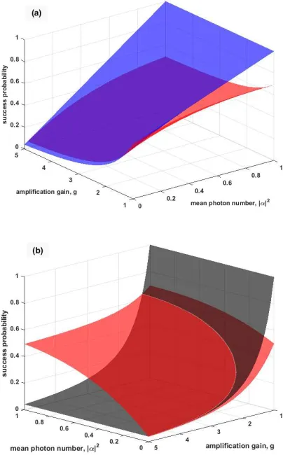
FIG. 3. (a) The exact success probability of a single QS (lower red),

Psucc, and that based on approximations in Ref. [18] (upper blue),

PRL

succ. (b) The exact success probability of a single QS (red),Psucc,

and that of an ideal NLA (grey),1/g2

, versus average photon number and amplification gain.

C. Probability of success

The probability of success for measurement Mˆ, PPS, is given by

PPS=Tr( ˆMρˆout)

=

Z _d2_ξ

1

π

Z _d2_ξ

2

π χ

out

A (ξ1, ξ2,0)[πδ2(ξ1)−1]. (13)

By substituting Eq. (7) into the above expression, we obtain

Psucc(α) = 2PPS(α)

=2−µ(1−|α| 2

2 )

e−|α|2/2−2(1−µ)e−|α|2,

(14)

wherePsucc(α)is the total probability of success for the QS module, i.e., when either of D1 or D2 detector clicks. As ex-pected,Psucc(α)approaches, to first-order approximation, to

PRL

succ(α) =µ+ (1−µ)|α|2 = (1 +|gα|2)/(1 +g2), when

|α| ≪ 1. This approximation is, however, invalid even when we slightly deviate from the condition on|α|, as can be seen in Fig.3(a). Here, we have plotted the exact probability of success,Psucc(α), versus|α|2 andg, and compared it with the asymptotic value obtained by Ralph and Lund,PRL

succ(α). It can be seen that the exact probability of success is always lower than the asymptotic value, and the difference is visi-ble at all values ofg. The success probability also increases with the decrease ing. For|α| ≪1, the success probability approaches its maximum possible value of1/g2 [17]. But, again, as can be seen in Fig.3(b), we quickly deviate from this ideal regime when|α|increases. This indicates that we cannot operate at maximum possible success probability for all possible inputs, as assumed in Ref. [15], if we use a QS as an NLA.

In Fig. 3(b), the maximum possible success probability,

1/g2_{, divides the plot into two regions. There is a region in} which the success probability is above the maximum possi-ble for an NLA. This implies that the QS operation should be very noisy in this region, hence breaking the assumption on the noise-free operation of the NLA. If we want to work in the region thatPsucc(α)<1/g2, we will then have to deal with limitations on the maximum gain that we can choose for the range of input states we may expect. This indicates a trade-off between the amount of noise that the QS may add to the signal versus its gain and success probability. We will later address this issue, in the context of CV QKD, in our numerical results when we optimize the secret key generation rate over system parameters.

D. Non-Gaussian behavior of the QS

Before calculating the secret key generation rate of a QS-equipped CV QKD system, it is necessary to better understand the nature of a quantum channel that includes a QS module. This is important because majority of results on the secret key rate of CV QKD systems rely on Gaussian characteristics of the channel [27,30]. This is not, however, the case for a QS module as we see in this section.

In order to examine the non-Gaussian behavior of the QS output, let us focus on the distribution of homodyne measure-ment results on quadraturexˆB. Let us also consider a loss-less

noise-free channel, which provides an input coherent state|αi, withα=xA+ipAas distributed by Eq. (1), at the QS port

ˆ

a1. The case of lossy and noisy channels will be considered in AppendixA. The probability distribution for obtaining a real numberxB after measuringxˆB, conditional on the

transmis-sion of|αiand the success of the QS, is then given by

fXB(xB|α) = Tr[|xBihxB|ρˆ PS out(α)]

=ρ00(α) + √

2 ρ01(α) +ρ∗01(α)

xB

+ 2ρ11(α)x2B

e−x2

B

√

π , (15)

-3 -2 -1 0 1 2 3 x

B

0 0.1 0.2 0.3 0.4 0.5

fXB (xB

)

output dist. Gaussian part non-Gaussian part

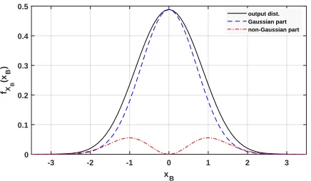
FIG. 4. The output distribution at the receiver side (solid-black), which comprises Gaussian (dashed blue) and non-Gaussian (dot-dashed red) parts. Here,g= 3andVA= 0.04.

states, we obtain

fXB(xB) =

Z

dxA

Z

dpAfXA(xA)fPA(pA)fXB(xB|α).

(16)

In the above expression, because fXA(xA)and fPA(pA) have zero-mean Gaussian distributions, the term ρ01(α) +

ρ∗

01(α)is averaged out after the integration in Eq. (16). The expression forfXB(xB)will then have two components: one is a Gaussian term in xB proportional to the average of

ρ00(α), and the other is a non-Gaussian term proportional to the average ofρ11(α). Figure 4 shows the contribution of each of these components in makingfXB(xB)forg= 3and

VA = 0.04. We notice that even for such a small

modula-tion variance, which corresponds mostly to small values of

|α|, the non-Gaussian term is quite distinct. Higher amplifica-tion gains could even result in more deviaamplifica-tion from a Gaussian state. This non-Gaussian behavior would have ramifications on the key rate analysis of a QS-based system as we see next.

IV. SECRET KEY RATE ANALYSIS

In this section, we use the results in Sec.IIIto determine the secret key rate of the GG02 protocol when Bob uses a single QS before his homodyne measurement. We find the secret key rate in a nominal operation condition when no eavesdropper is present. We assume a thermal loss channel with trasmissivity

T, modeled by a beam splitter, and an excess noise,ε, at the input of the channel. The secret key rate of CV QKD proto-cols in the asymptotic limit of infinitely many signals is given by

K=βIAB−χBE, (17)

whereβ, IAB, χBE are, respectively, the reconciliation

effi-ciency, the mutual information between Alice and Bob, and eavesdroppers accessible information when reverse reconcili-ation is used.

In our proposed setup, since the QS operation is non-deterministic, the whole key rate formula should be multiplied

by theaveragesuccess probability of the QS,Psucc, where the averaging is performed over all possible inputs. Therefore, the secret key rate reads

KQS≥Psucc(βIAB⋆ −χ ⋆

BE), (18)

where ‘⋆’ indicates that the mutual and Holevo information terms are calculated for the post-selected data when the QS is successful. The measurement results corresponding to unsuc-cessful QS events will be discarded at the sifting stage.

The fact that we only use the post-selected data for key extraction implies that we have to account for the Gaussianity of the QS output states. Unfortunately, the non-Gaussian behavior of the QS makes conventional methods for key rate calculation inapplicable. In order to take the non-Gaussian effects into account, we calculate the exact mutual information by directly using the conditional distribution of the QS output. Ideally one could also look for the exact cal-culation of the Holevo information term as well. But, this turns out to be extremely cumbersome. Instead, in this paper, we find an upper bound for the Holevo information term by finding the covariance matrix (CM) of the actual channel and then calculate the Holevo information for a Gaussian channel with the same CM. The reason is that Gaussian collective at-tacks for a given CM is proven optimal in the sense that they maximize the Holevo quantity [30]; hence, providing a lower bound on the key rate.

In the following, we provide more detail on how each of the terms in Eq. (18) can be calculated.

A. Mutual information

The mutual information between two random variablesXA

and XB, corresponding, respectively, to post-selected data

on Alice and Bob side, is, by definition, the difference be-tween the entropy functionH(XB)and the conditional

en-tropyH(XB|XA)[31]:

IAB⋆ =H(XB)−H(XB|XA), (19)

where

H(XB) =−

Z

dxBfXB(xB) log2fXB(xB), (20)

and

H(XB|XA) =−

Z

dxAfXA(xA)

×

Z

dxBfXB(xB|xA) log2fXB(xB|xA),

(21)

with

fXB(xB|xA) =

Z

dpAfPA(pA)fXB(xB|xA+ipA). (22)

50/50

EPR BS

BS BS

D2

D1

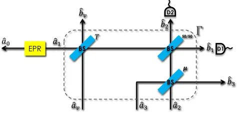
FIG. 5. QS-amplified EB CV QKD scheme. The quantum channel and the QS are considered as a combined system with input modes

ˆ

a1₋ˆa3andˆavand three output modesˆb1₋ˆb3andˆbv. The

trans-formation matrix of the system is given by Eq. (23).

noise; see AppendixAfor details. In our work, we numeri-cally carry out the above integrals for a given set of parame-ters.

B. Holevo information

In order to calculate the Holevo information term,χ⋆ BE, we

use the EB description of the protocol, where one part of an EPR state travels through the quantum channel and amplified by a QS, while the other is measured by Alice; see Fig.5. In order to upper boundχ⋆

BE, what we need is then the CM of

Alice-Bob bipartite state. We will then first derive the exact post-selected joint state, from which the CM parameters can be obtained.

We use a similar approach to Sec. IIIin using character-istic functions to find a relationship between Alice and Bob states when the QS is successful. As shown in Fig. 5, we also account for the effect of the quantum channel in our cal-culations. Note that the dashed box in Fig.5is a linear op-tics circuit, for which input-output relationships can be ob-tained. In particular, considering the input modes represented byAT _{= [ˆa}

1aˆ2ˆa3ˆav]and output modesBT = [ˆb1ˆb2ˆb3ˆbv],

we findB= ΓA, where the transformation matrix

Γ =

     

q

T

2

pµ

2 −

q

1−µ

2

q

1−T

2

−qT

2

pµ

2 −

q

1−µ

2 −

q

1−T

2

0 √1−µ √µ 0

−√1−T 0 0 √T

     

(23)

is a unitary matrix.

By using Eq. (2) and the transformation matrixΓ, we can now write the full output anti-normally ordered characteris-tic function, includingˆa0mode, in terms of the input one by

χout

A (ξ0, ξ1, ξ2, ξ3, ξv) =χinA(λ0, λ1, λ2, λ3, λv), where

[λ0λ1λ2λ3λv]T =

1 0 0 ΓT

[ξ0ξ1ξ2ξ3ξv]T, (24)

withP_j|λj|2=Pj|ξj|2and

χinA(λ0, λ1, λ2, λ3, λv) =χEPRA (λ0, λ1)×χinA(λ2, λ3, λv),

(25)

where χEPR

A (λ0, λ1) = exp{−δ2(|λ0|2 + |λ1|2) −

2Re(δγλ∗

0λ∗1)} is the anti-normally ordered characteristic function of the EPR state with parameters δ and γ =

√

δ2_{−1, Re[ξ] being the real part of the complex} num-ber ξ, and χin

A(λ2, λ3, λv) is calculated for an input state |1iˆa2|0iaˆ3|0iˆav. Putting all this together, we then find the pre-measurement anti-normally ordered characteristic func-tion for modesaˆ0,ˆb1,bˆ2,ˆb3, andˆbvas follows:

χoutA (ξ0, ξ1, ξ2,ξ3, ξv) =e−δ 2

|ξ0|2_e−ωRe ξ∗0(ξ∗1−ξ∗2)

×e−δ

2_T

2 |ξ1−ξ2−√2τ ξv|2_e−1−2T|ξ1−ξ2+

√

2

τ ξv|2

×e−1−2µ|ξ1+ξ2−

√₂

g ξ3|2_e−µ₂|ξ1+ξ2+√2gξ3|2

×1−µ₂|ξ1+ξ2+ √

2gξ3|2

, (26)

where g = p(1−µ)/µ, τ = p(1−T)/T , and ω = 2δγpT /2. Note that we account for the effect of excess noise by adjusting the effective modulation variance as de-scribed in AppendixA.

Having obtained the characteristic function, we can find the corresponding output density matrix using Eq. (3). Then, by tracing out the output modeˆbv and also performing

photon-detection measurements on modesˆb1andˆb2—by introducing the same measurement operator as in Eq. (9)—we find the resultant joint state ofˆa0andˆb3modes in the case of having a successful event.

AppendixBprovides the detailed calculations of the post-measurement density matrix, and the corresponding CM pa-rameters. It turns out that the CM of the shared bipartite state between Alice and Bob has the form

γAB =

a1 cσz

cσz b1

, (27)

a=−1− 2

(g2_{+ 1)P} succ

_4δ2_[γ2_{T −(2F+ 1)][(2F+ 1)g}2_{+ 2F]−4δ}2_γ2_T

(2F+ 1)3 −

δ2_g2_(γ2_T−2F)

2F2

,

b=−1− 2

(g2_{+ 1)P} succ

−4[g

2_{(2F+ 1) + 2F]}

(2F+ 1)2 −

4g2

2F+ 1 + 2g2

F

,

c= 8δγg

√

T (g2_{+ 1)(2F+ 1)}2_P

succ

, (28)

and

F = 1−T+δ

2_T

2 and Psucc= 2 g2_{+ 1}

_{2[(2F+ 1)g}2_{+ 2F]}

(2F+ 1)2 −

g2

2F

.

It is interesting to make the following observation. If the EPR state is assumed totally uncorrelated, which happens when its squeezing parameter goes to zero, both parts of the state are left with vacuum states. Thus, if the QS is successful, the output state of modeˆb3should be a vacuum state as well. This means that the CM of the end-to-end state is identity [8]. We verify that in the case of having a totally uncorrelated EPR state, corresponding to δ = 1 andγ = 0, the expressions above will indeed result in the identity matrix; that is, we ob-taina=b= 1andc= 0.

Now that the CM is known, we can upper bound the Holevo information by using Eq. (B13).

V. NUMERICAL RESULTS

In this section, we present numerical simulations of the se-cret key rate of the QS-amplified GG02 protocol and compare it with that of the conventional one. We find the maximum value for the lower bound in Eq. (18) by optimizing, at each distance, the modulation variance, VA, or, equivalently, the

parameterδin the EB scenario, as well as the QS parameter,

µ, which specifies the QS amplification gain. We also account for the excess noise which, as discussed in AppendixA, can be included in the modulation variance. We assume that the quantum channel between the sender and receiver is an opti-cal fiber with loss factorα, whose transmittance is given by

T = 10−αL/10

, whereL is the channel length and the loss factor is α = 0.2 dB/km corresponding to standard optical fibers. Also, we assumeβ = 1and that ideal homodyne de-tection, with no electronic noise, is performed at the receiver.

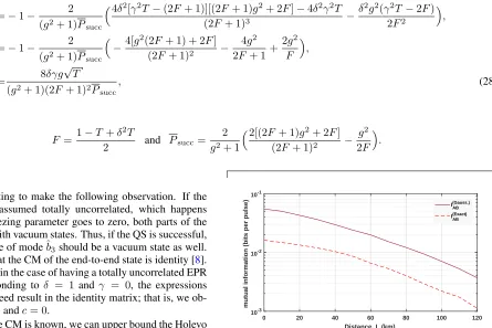
We first highlight the importance of accounting for the non-Gaussian behavior of the QS by comparing the difference be-tween the exact value of the mutual information functionI⋆

AB,

given by Eq. (19), and that obtained by Gaussian approxima-tion, IG

AB, in Eq. (B14). Figure 6 shows both curves,

ver-sus distance, at no excess noise. It is clear that the Gaus-sian approximation would have overestimated the mutual info between Alice and Bob at all distances considered, and that could have resulted in wrong bounds for the key rate of QS-based systems.

0 20 40 60 80 100 120

Distance, L (km) 10-3

10-2 10-1

mutual information (bits per pulse)

I_AB(Gauss.)

I_AB(Exact)

FIG. 6. The exact mutual information function (dashed) as compared to its Gaussian approximation (solid) versus distance atε = 0. All other parameters have been optimized.

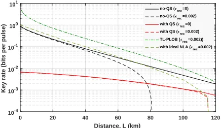
Figure7shows the optimized secret key rates of both con-ventional and the QS-assisted GG02 protocol versus distance in two scenarios: with and without excess noise. In the case of no excess noise, it can be seen that the no-QS curve stays above the QS-assisted system at all distances considered. The slope of the QS-based system is, however, almost half of the no-QS system, especially at short to mid range distances, which resembles a repeater behavior. By introducing a fixed excess noise of 0.002 at the receiver, the QS-based system of-fers a clear rate advantage over distances greater than 80 km, and can reach a security distance of around 120 km. This is a promising result in the sense that one extend the range of CV QKD systems by nearly 50% using a simple QS module. More importantly, the better rate-versus-distance scaling of the QS-assisted system makes it a potential candidate for CV repeater setups [25].

As can be seen in Fig.7, QS-equipped receivers may not support high key rates at short distances. There are over two orders of magnitude difference between the no-QS and QS-based curves atL = 0. This is attributed to multiple factors. First, the trade-off between the choice of modulation variance and noise level in the system, would require us to use very small values ofVAat short distances, as otherwise, the QS will

no-0 20 40 60 80 100 120 Distance, L (km)

10-4 10-3 10-2 10-1 100 101

Key rate (bits per pulse)

no-QS (rec=0)

no-QS (rec=0.002)

with QS (rec=0)

with QS (rec=0.002)

TL-PLOB (rec=0.002))

with ideal NLA (rec=0.002)

FIG. 7. The optimized secret key rate for the QS-amplified CV QKD protocol versus distance, as compared to the rate of conventional GG02, the upper bound for a thermal-loss channel (TL-PLOB) at a mean thermal photon number ofεrec/(2(1₋T)), and the rate

ob-tained by an ideal NLA.

TABLE I. Optimized values for modulation variance and amplifica-tion gain at zero excess noise.

Distance (km) Optimized modulation variance Optimized gain

0 0.05 1.02

50 0.20 1.36

100 0.45 1.53

QS system with such a low value ofVAalso offers a low key

rate of3.52×10−2_{, which is comparable to what we obtain} for the QS-based system. Other factors are the success prob-ability, which atL = 0is around 0.5, and it almost linearly goes down to around 0.2 at 120 km. One other factor is also the fact that the QS is not entirely noise free. The additional noise by the QS would bring the rate atL= 0to around 0.01 per pulse.

The post-selection mechanism in the QS is the key to ob-taining higher key rates at long distances. At long distances, the channel loss naturally prepares low-intensity inputs to the QS, which allows us to use larger values ofVA, as shown in

TableI. That would also enable us to use slightly higher gains without necessarily increasing the QS noise. A higher-than unity gain for the post-selected states would then offer a bet-ter signal-to-noise ratio at long distances, which allows us to achieve positive secret key rates at longer distances. It is note-worthy that, atεrec = 0.002, the maximum security distance that can be achieved by using an ideal NLA, as in Ref. [15], is almost the same as we have achieved with the QS. This im-plies that within certain regions the QS module can offer a performance close to ideal NLA devices, which matches our findings in Sec. III. Note that the plots in Ref. [15] are ob-tained for fixed values of amplification gain and modulation varianceg = 4andVA = 3.5, respectively), where no

op-timization is performed. The ideal NLA curve in Fig. 7 is, however, gained after optimizing the secret key rate given in Ref. [15].

Figure7 also shows that our QS-amplified system cannot beat the existing upper bounds for repeaterless systems [32]. Here, we have used the bound given in Eq. (23) of Ref. [32]

for a thermal-loss channel as a benchmark (labelled TL-PLOB in Fig.7). This curve has been obtained at an equivalent mean thermal photon number,n¯, to our receiver excess noise. That is, we have usedn¯ = εrec/(2(1−T)). As expected, the QS-based system cannot outperform this bound. This again indicates that one would need a CV repeater setup in order to beat such bounds by CV QKD.

VI. CONCLUSIONS AND DISCUSSION

In this work, we studied the performance of the GG02 pro-tocol where the received signal was amplified by a quantum scissor. We first obtained the exact output state and success probability of the QS under study, which was latter used in calculating the secret key generation rate of the system. We showed that the QS would turn a Gaussian input state into a non-Gaussian one. That would make the conventional tech-niques to estimating the key rate not directly applicable to our case. We instead directly calculated the mutual informa-tion by working out the probability distribuinforma-tion funcinforma-tion of the quadratures after the QS. Also, in order to upper bound the leaked information to Eve, we obtained the exact covari-ance matrix of the bipartite state shared between sender and receiver labs. We then found the Holevo information corre-sponding to a Gaussian channel with the same covariance ma-trix. We optimized the key rate over input modulation vari-ance and amplification gain. Our results showed that the QS-enhanced key rate can tolerate more excess noise than the no-QS system. This implied that we could reach longer distances, up to 120 km with existing technologies, by using a QS at the receiver module.

the signal level by optimizing the modulation variance.

ACKNOWLEDGMENTS

The authors acknowledge partial support from the White Rose Research Studentship and the UK EPSRC Grant No.

EP/M013472/1. All data generated in this paper can be re-produced by the provided methodology and equations.

Appendix A: Channel loss and excess noise

In order to calculate the exact conditional and marginal entropy functions in Eqs. (20)–(22), the following procedure should be followed:

Channel transmittance (T). The state that reaches the QS is attenuated because of the channel transmittance; hence, in Eqs. (15) and (16):(xA, pA)→(

√

T xA, √

T pA).

Channel excess noise (ε). A thermal excess noise that is added at the channel input can be modeled by an independent Gaussian distribution. In the prepare and measure scheme, that implies that the effective modulation variance of the system should change fromVA toVA+ε. This is because the sum of two independent Gaussian distributions is another Gaussian

distribution with a variance equal to the sum of their variances [31]. In the EB scheme, we find the corresponding parameterδin our EPR state, which gives the same output statistics for the signal that goes to Bob, when Alice does a heterodyne measurement on her state. It then turns out that to get an identical output state we should satisfyδ=p(V + 1)/2, whereV =VA+ε+ 1.

Note that in our simulation, following the experimental results in Ref. [9], we assume that the noise level,εrec, is measured at the receiver. We estimate the excess noise at the transmitter side byε=εrec/T.

Appendix B: Covariance matrix

Having obtained the output anti-normally ordered characteristic function of Eq. (26), we use Eq. (3) to find the corresponding output state:

ˆ ρout0123v=

Z _d2_ξ

0

π d2_ξ

1

π d2_ξ

2

π d2_ξ

3

π d2_ξ

v

π χ

out

A (ξ0, ξ1, ξ2, ξ3, ξv) ˆDN(ˆa0, ξ0) ˆDN(ˆb1, ξ1) ˆDN(ˆb2, ξ2) ˆDN(ˆb3, ξ3) ˆDN(ˆbv, ξv). (B1)

In the following, we show how the shared state between Alice and Bob is found step-by-step. We first trace out modebv, see

Fig.5, to obtain

ˆ ρout0123=

Z _d2_ξ

0

π d2_ξ

1

π d2_ξ

2

π d2_ξ

3

π χ

out

A (ξ0, ξ1, ξ2, ξ3,0) ˆDN(ˆa0, ξ0) ˆDN(ˆb1, ξ1) ˆDN(ˆb2, ξ2) ˆDN(ˆb3, ξ3), (B2)

where we useTr[ ˆDN(a, ξ)] =πδ2(ξ). Next, by defining the measurement operatorMˆ = (I− |0ib1h0|)⊗ |0ib2h0|, modesˆb1

andˆb2are measured. The post-selected state is

ˆ ρPS03 =

Tr12[ ˆMρˆout0123]

Tr[ ˆMρˆout 0123]

=: ˆσ

PS 03

PPS EB

, (B3)

where

ˆ σ03PS=

Z _d2_ξ

0

π d2_ξ

3

π

" Z _d2_ξ

1

π d2_ξ

2

π χ

out

A (ξ0, ξ1, ξ2, ξ3,0) πδ2(ξ1)−1

#_ˆ

DN(ˆa0, ξ0) ˆDN(ˆb3, ξ3)

=

Z _d2_ξ

0

π d2_ξ

3

π χeA(ξ0, ξ3) ˆDN(ˆa0, ξ0) ˆDN(ˆb3, ξ3) (B4)

with the following definition

e

χA(ξ0, ξ3) :=

Z _d2_ξ

1

π d2_ξ

2

π χ

out

andPPS

EB =Psucc/2is the corresponding success probability to measurementMˆ:

PEBPS=

Z _d2_ξ

1

π d2_ξ

2

π χ

out

A (0, ξ1, ξ2,0,0) πδ2(ξ1)−1

=χeA(0,0). (B6)

Now, we find the CM forρˆPS

03. In doing so, we need to work out the triplet(a, b, c)of the corresponding CM as follows. By definition, assuming thatxˆ0is theXquadrature of modeˆa0, we have

a=hxˆ20iρˆ03 =

hxˆ2 0iσˆ03

PPS EB

= Tr[ˆx

2 0σˆ03]

PPS EB

, (B7)

where

Tr[ˆx20σˆ03] =

Z _d2_ξ

0

π d2_ξ

3

π χeA(ξ0, ξ3)×Tr[ˆx

2

0DˆN(ˆa0, ξ0)]×Tr[ ˆDN(ˆb3, ξ3)]

=

Z _d2_ξ

0

π χeA(ξ0,0)×Tr[ˆx

2

0DˆN(ˆa0, ξ0)]. (B8)

Assuming thatξ0=x+iy, one can show thatTr[ˆx20DˆN(ˆa0, ξ0)] =πδ2(ξ0) + 2πyδ(x)_dydδ(y)−πδ(x)d

2

dy2δ(y); thus,

Tr[ˆx20σˆ03] =−χeA(0,0)−

d2

dy2χeA(0, y, ξ3= 0)

y=0, (B9)

where we use the identityR dzf(z)_dzdδ(z) =−Rdz_dzdf(z)δ(z). Therefore,

a=−1−

d2

dy2χeA(0, y, ξ3= 0)

y=0

e

χA(0,0)

. (B10)

In a similar way, assumingξ0=x+iyandξ3=u+iv, we show that

b=Tr[ˆx

2 3σˆ03]

e

χA(0,0)

=−1−

d2

dv2χeA(ξ0= 0,0, v)

_v=0

e

χA(0,0)

(B11)

and

c= Tr[ˆx0xˆ3σˆ03]

e

χA(0,0)

=

d dv

h

d

dyχeA(0, y,0, v)

y=0

i

v=0

e

χA(0,0)

. (B12)

Having the integrals in Eq. (B5) taken, we are able to calculate the triplet(a, b, c), thus the CM. UsingMAPLE, we obtain the closed form expressions as summarized in Eq. (28).

Having the triplet(a, b, c),χ⋆

BEis upper bounded by:

χGBE =g(Λ1) +g(Λ2)−g(Λ3), (B13)

where

g(x) = (x+ 1 2 ) log2(

x+ 1 2 )−

x−1 2 log2

x−1 2

and

Λ1/2=

r

1 2 A±

p

A2_−4B2 ₌

p

(a+b)2_−4c2 _±(b−a)

2 , Λ3=

r

aB b =

r

a(ab−c2₎

b ,

withA=a2_+b2_−2c2_andB=ab−c2_{. Note that Eq. (B13) is valid when we neglect the electronic noise at the receiver as} we have assumed in our numerical results. Also, mutual information can be calculated form the covariance matrix, if we wish to use the Gaussian approximation, by

IABG =

1 2log2

ab

ab−c2. (B14)

[1] C. H. Bennett and G. Brassard, inProceedings of IEEE Interna-tional Conference on Computers, Systems, and Signal

[2] A. K. Ekert,Phys. Rev. Lett. 67, 661 (1991).

[3] N. Gisin, G. Ribordy, W. Tittel, and H. Zbinden, Rev.

Mod. Phys.74, 145 (2002).

[4] V. Scarani, H. Bechmann-Pasquinucci, N. J. Cerf, M. Duˇsek, N. L¨utkenhaus, and M. Peev,Rev. Mod. Phys.81, 1301 (2009). [5] F. Grosshans and P. Grangier, Phys. Rev. Lett. 88, 057902

(2002).

[6] F. Grosshans, G. Van Assche, J. Wenger, R. Brouri, N. J. Cerf, and P. Grangier,Nature421, 238 (2003).

[7] S. L. Braunstein and P. van Loock,Rev. Mod. Phys.77, 513

(2005).

[8] C. Weedbrook, S. Pirandola, R. Garc´ıa-Patr´on, N. J. Cerf, T. C. Ralph, J. H. Shapiro, and S. Lloyd,Rev. Mod. Phys.84, 621

(2012).

[9] P. Jouguet, S. Kunz-Jacques, A. Leverrier, P. Grangier, and E. Diamanti,Nat. Photon.7, 378 (2013).

[10] S. Pirandola, C. Ottaviani, G. Spedalieri, C. Weedbrook, S. L. Braunstein, S. Lloyd, T. Gehring, C. S. Jacobsen, and U. L. Andersen,Nat. Photon.9, 397 (2015).

[11] T. Hirano, H. Yamanaka, M. Ashikaga, T. Konishi, and R. Namiki,Phys. Rev. A68, 042331 (2003).

[12] H. Yonezawa, S. L. Braunstein, and A. Furusawa,Phys. Rev.

Lett.99, 110503 (2007).

[13] S. Yokoyama, R. Ukai, S. C. Armstrong, C. Sornphiphatphong, T. Kaji, S. Suzuki, J. ichi Yoshikawa, H. Yonezawa, N. C. Menicucci, and A. Furusawa,Nat. Photon.7, 982 (2013). [14] P. Jouguet, S. Kunz-Jacques, and A. Leverrier,Phys. Rev. A

84, 062317 (2011).

[15] R. Blandino, A. Leverrier, M. Barbieri, J. Etesse, P. Grangier, and R. Tualle-Brouri,Phys. Rev. A86, 012327 (2012). [16] Y.-C. Zhang, Z. Li, C. Weedbrook, S. Yu, W. Gu, M. Sun,

X. Peng, and H. Guo, J. Phys. B: At. Mol. Opt. Phys. 47,

035501 (2014).

[17] S. Pandey, Z. Jiang, J. Combes, and C. M. Caves,Phys. Rev. A

88, 033852 (2013).

[18] T. C. Ralph and A. P. Lund,AIP Conference Proceedings1110,

155 (2009).

[19] E. Eleftheriadou, S. M. Barnett, and J. Jeffers,Phys. Rev. Lett.

111, 213601 (2013).

[20] J. Fiur´aˇsek,Phys. Rev. A80, 053822 (2009).

[21] G. Y. Xiang, T. C. Ralph, A. P. Lund, N. Walk, and G. J. Pryde,

Nat. Photon.4, 316 (2009).

[22] F. Ferreyrol, M. Barbieri, R. Blandino, S. Fossier, R. Tualle-Brouri, and P. Grangier,Phys. Rev. Lett.104, 123603 (2010). [23] R. J. Donaldson, R. J. Collins, E. Eleftheriadou, S. M.

Bar-nett, J. Jeffers, and G. S. Buller,Phys. Rev. Lett.114, 120505

(2015).

[24] M. Barbieri, F. Ferreyrol, R. Blandino, R. Tualle-Brouri, and P. Grangier,Laser Phys. Lett.8, 411 (2011).

[25] J. Dias and T. C. Ralph,Phys. Rev. A95, 022312 (2017). [26] F. Furrer and W. J. Munro, arXiv:1611.02795.

[27] J. Lodewyck, M. Bloch, R. Garc´ıa-Patr´on, S. Fossier, E. Kar-pov, E. Diamanti, T. Debuisschert, N. J. Cerf, R. Tualle-Brouri, S. W. McLaughlin, and P. Grangier,Phys. Rev. A76, 042305

(2007).

[28] R. Kumar, H. Qin, and R. Allaume,New J. of Phys.17, 043027

(2015).

[29] M. A. Nielsen and I. L. Chuang, Quantum Computation and Quantum Information(Cambridge University Press, Cam-bridge, 2000).

[30] R. Garc´ıa-Patr´on and N. J. Cerf,Phys. Rev. Lett.97, 190503

(2006).

[31] T. M. Cover and J. A. Thomas,Elements of Information Theory-Second Edition(John Wiley and Sons, New Jersey, 2006). [32] S. Pirandola, R. Laurenza, C. Ottaviani, and L. Banchi,Nat.

Commun.8, 15043 (2017).

[33] M. M¨uller, S. Bounouar, K. D. J¨ons, M. Gl¨assl, and P. Michler,

Nat. Photon.8, 224 (2014).