On the distribution of queueing times for queues with two servers

On the Distribution of Queueing Times for

Queues with Two Servers by

N.M.H. Smith

A Thesis prepared for the Degree of Doctor of Philosophy At Australian National University during the period from

Preface

(i)

The work of this Thesis arose from a very natural, although really quite accidental drawing together of ideas from two completely separate fields of academic endeavour.

On one side, the Probabilitists had progressed quite well with most of those classes of queueing problems which could be reduced to equivalent random walks on the line, but only a very limited success had been achieved with those queues of

the GI/G/C class which were such that the equivalent walks were of necessity over multivariate real space. Moreover, such progress as appeared to have been made was embodied in the incomplete and apparently very difficult works of Pollaczek.

On the other hand, this century has seen much progress in a branch of analysis which was little explored before the end of

the nineteenth and which is, it seems, still too new to be taught to undergraduates or, to labour a point, undergrad­ uate probabilitists. Thus it was for me quite shocking to discover the existance of that vast and profoundly useful structure which is Multivariate Complex Analysis and to begin to dimly see that therein might lie a key to the general Multidimensional Random Walk.

(iü) Acknowledgements

Many people have helped me both directly and indirectly in the preparation of this Thesis but I should particularly like to thank the following:

(i) My Supervisor, Professor P.A.P. Moran for his many kindnesses and most valuable and diligent criticisms. (ii) Dr. D. Vere-Jones who first introduced me to the

Wiener-Ilopf method and later deduced the ergodic limiting bivariate distribution for the M/M/2 Queue by probabi­ listic means, thereby verifying some of the results.

(iii) Drs. N.E. Day, C. Heathcote and P. Mandl for useful advice, stimulation and copies of papers at various times.

(iv) Emeritus Professor E. Hille who in a most brief yet useful conversation drew my attention to the works of Salomon Brochner and thence indirectly to the apparatus which is Multivariate Complex Analysis.

(v) Mrs. B. Cranstone, Mrs. W. Hunt and Mrs. K. Strickland for the accurate typing of some most illegible drafts. (vi) The Australian Public Service Board and Post Master

General's Department for their financial assistance in the form of a two year Commonwealth Public Service Scholarship, which permitted me to spend this time at A.N.Ü. working on this Thesis.

Certification

Except at those points where I have specifically indicated otherwise or where I have used a suitably named Theorem, the work of this Thesis is the result of my own efforts aided only by the numerous criticisms of my supervisors.

( V )

PRECIS

Initially we consider first come first served queues with two or more servers wherein the intervals between the

successive arrivals are independently and identically distributed. The customers1 service times are similarly distributed.

The method is to define an embedded Markov chain on the moments just before each arrival and thence recurrences ^ which prelate the state of the system just before the (n+1; arrival to that which existed just before the nth. The

problem is then specialized to that for two servers and these probability recurrences are used to develop a relationship between the bivariate Laplace transformations of the

distribution functions which arise.

The problem is reduced to the solution of a single integral equation for the Laplace transformation of the ergodic limiting distribution function by the definition of two compensation functions. These steps are analogous to the veil known probability "sweeping up" operations for one server queues.

This integral equation is reduced to a functional equation for the case where the interarrival and service

tine distributions are both composed of any integral numbers of exponential stages. This equation is solved in principle for all finite numbers of such stages, and in detail when the service time distribution has one or two stages and the interarrival time distribution any number.

The results are checked against a known result for one case and a set of simulation results for another. The

agreement is satisfactory.

Of particular note are the curious loci of certain singularities.

The Thesis also discusses a number of important intermediate results which suggest that the classical Miener-Kopf method for a unidimensional integral equation may generalize to a useful multidimensional result. We

(Vi)

Contents Pa£e

1. Glossary of Notation

1.1 L a t m

1

1.2 Greek 13

2. Two Alternative Markov Processes for GI/G/2

2.1 Assumptions 19

2.2 Development of the First Markov Process 20

2.3 The Second Markov Chain 24

3. The Analagous Markov Processes for GI/G/C 31

4. Laplace Stieltjies Transforms 33

Excursus On the One Server Wiener-Hopf Method 36 " The Kiefer & Wolfowitz Conditions for 45

GI/G/C

5. Preliminary Definitions and Theorems

5.1 Definitions 49

5.2 Standard Theorems 53

6. Properties of Transforms 64

*

6.1 First Region of Continuity of x+ ($>0 ) 6 5 *

6.2 First Domain of Analyticity of x+C^»0 ) °° /If

The Definition of (0) and (0) 6 8

^ A

Excursus - The Analogue of 7T^ (0) for the

One Server Queue 69

6.3 Limit Re(4>)-*» of X * ( < M ) 72 6.4 If A(a) is absolutely continuous the line

x=0 ye(0,°°) is a set of probability measure

(vii)

6.5 First Domain of Analyticity of tt^ (9) and 76

TT^Ce) 76

k

6.6 First Region of Continuity of ^ (<*>»©) 9 3 *

6.7 First Domain of Analyticity of x (<J>,0) 95 *

6.8 Limit Re(<J>)-*» of y (<^,0) 96 *

6.9 Limit Re(0)-»— <» of y (£,9) 99 *

The Definition of x_+(4>»0) 101

6.10 First Domain of Analyticity and First Region

. *

of Continuity of y ( ($,6) 101

Definitions of x CO»0) 105

k

6.11 Continuity and Analyticity of x (0»9) 105 6.L2 Limit Re((J>)-*-«> of x ($»6) 112 6.L3 x!<0,9) - X*_(0,9)

wherever these exist. 113

k

6.L4 Continuity and Analyticity of y+ (-y,vi+Q)) 116 k

6.15 Continuity and Analyticity of y^C-vuu+G+cl)) 117

6.16 Limit Re((o)-*-«^x*(~y,y+w) 118

•fa

6.17 Continuity and Analyticity of y+ (z-y,y-KA)-z) 119 6.10 Limit Re(z)-*“00 of X+ (Z“U,y-Ko-z) 120 6.19 Limit ReC©)*»00 of X+ (0>0) 12 3 Definition of a Singularity Locus 126

*

6.20 Singularities of y^C-yjU+w) 126

6.21 (i) Singularity Loci of D ^{x+ (z-y»y+w“z)|!=o

131

(v34i)

6.21 (ii) Continuity of D ^ ^ C z - y ,y-Ho-z) )=0

for j *

1

,

2

, . . .

6.22 Limit Re<w)-*»/D 3(x. (z-y.p+w-z)} _

A z + z *U

for j = 1,2,... 133

7. Ergodic Functional Equations for the E^/E^/2 Queue

The Definitions of the Centre Function C(cj>,0) 136 8. Ergodic Functional Equations for the Queues

M/M/2 E2/E2/2

V V

2

140

9. The Nature of C(0,0)

9.1 Preliminary Lemmae 141

9.2 Partial Analytic Continuation 142

9.3 Representation Theorems 145

9.4 C(f (40 ,w-f (a))) = M(f (w) ,0D~f (O)))

for all u) iff f(u)) is suitably defined 152 9.5 Extension of the first domain of analyticity

of d^+ ^(0) for m = l,2,...,k

m 155

9.6 The d^*^(0) are all entire whence C($,0) is m

entire 158

9.7 C(<£,0) is a Bivariate Polynomial (for

V V 2>

162

( ix )

12. The S o l u t i o n o f E /M/2 f o r K * 1 , 2 , . . .

K.

Excursus - Check S o l u t i o n o f M/M/2

13. The S o l u t i o n o f f o r K = 1 , 2 , . . .

14. Summary o f E q u a t i o n s f o r

15. Sample S o l u t i o n o f E^/ E^l 2 and S i m u l a t i o n Check

15.1 T h e o r e t i c a l V a lu e s

15.2 The S i m u l a t i o n s

15.3 C om parisons o f r e s u l t s

16. I n t e r p r e t a t i o n s and C o n j e c t u r e s

16.1 System s o f t h e E /E /2 C l a s s K. Li

1 6 . 1 . 1 Forms o f S o l u t i o n s

1 6 . 1 . 2 U n iq u e n e s s o f S o l u t i o n s

1 6 . 1 . 3 The Meaning o f t h e S i n g u l a r i t i e s

16.2 The Queue GIxC/G/1

17. A C o n t i n u a t i o n a n d C o m p l e t i o n T h e o r e m

R e f e r e n c e s

A p p e n d i x l 1 1 1^ ^ 2 / 12 ^ S i m u l a t i o n P r o g r a m m e

A p p e n d i x I I T h e M e t h o d s o f F . P o l l a c z e k

184

190

194

215

217

220

222

226

231

(X)

Summary

The work was taken up from the following background;

1. Except for such special cases as GI/M/C and M/D/C, there existed no complete results for the queues of the GI/G/C class. Partial analytic results appeared to be available, however, from the incomplete work of Pollaczek, but

nobody had been able to carry out the apparently finite number of algebraic operations required to obtain a specific result for any case where the Laplace Transformation of the Service Time Distribution was rational.

2. Almost innumerable papers exist on queues of the GI/G/1 class based on a wide variety of methods. However, Kingman has shown in [9], that all of these methods were in essence,

identical. Furthermore, he had related all of these to Wendel’s paper on the Theory of Projective Operatdts.

3. Kingman had also noticed a certain inherent weaknesses in the probabilistic basis of the Pollaczek method for the GI/G/C queue which only arises if C>2. See Kingman [sTJ paragraph 12. 4. During the discussion of a paper by Pollaczek [15] , Weiss

had suggested that it might be better to try to apply the notions of the Wiener-Hopf method to queues of the GI/G/C class rather than to proceed as it seemed to him Pollaczek was doing, backwards from an assumed form of solution. 5. I was introduced to the traditional Wiener-Hopf apparatus

(Xi)

the solution of GI/G/1 class queues in terms of Compensation Functions and immediately saw that it would be easy to find rules with which to construct the multidimensional compen­ sation functions for multi-server queues.

The following connected sequence of investigation was put in hand;

1. The verification of Kingman's comment on Pollaczek’s work. 2. The reformulation of the problem in such a way that any

ambiguity if it existed, was overcome.

3. To apply to that formulation those perhaps more pedestrian analytic methods based on the use of Compensation Functions rather than the multidimensional Complex Integrals of unit steps at the origins on the real lines, in order to ‘’sweep u p “ the probabilities associated with negative variables. Remarks;

(i) Trivially, the two processes are equivalent, if they are correct, but one may reasonably expect that if one constructs a compensation function (or functions) in accordance with some pre-deduced rules, one may then be able to determine the analyticity and continuity properties of this function

(or those functions) with the aid of those rules. Also, it is clear that since these are rules for “sweeping u p “ probabilities they must be unique.

Transfor-(xii)

mation space) iterations. Naturally,this leads him straight into C simultaneous integral or functional equations for the C server queue.

(iii) Furthermore one is then left with these simultaneous

equations to solve and all that one knows is that the ergodic limiting probabilistic solution must, if it exists at all, be a C dimensional symmetric distribution function (with C dimensional symmetry) if the queue has C servers.

To obtain an equation or equations applicable to the simplest general multi-server queue, namely GI/G/2 which would be as closely analagous to the Wiener-Hopf - W.L. Smith equation for GI/G/1 as might be possible.

5 Obtain the equations to be solved for the ergodic limiting distributions in some of the simpler cases.

@ To solve these and verify the solutions by some independent means.

To consider the general implications of the work and any additional work which appears necessary.

The following thesis is the connected record of this work, arranged in seventeen Sections and two Appendices. For reasons of continuity, the verification of Kingman’s comment on, and my own comments on the Pollaczek method are placed in Appendix

II, but the remainder has been presented in the order in which it was carried out. Thus after Section 1 which is a glossary of the main notation we find;

(xiii)

random walks which correspond with the embedded Markov chain of the queue GI/G/2, and the recurrences which define these walks.

2. Section 3 outlines the alternative recurrences for the equivalent walks for the queue GI/G/C in terms of two ordered set of variables > .... > vc ^ VC where

£ = max (0,VC) * W where W is the Waiting Time, and

(+)

„

(+) „<+)

„

(+)

V1

^V 2

* ,,,,2 vc-l ^ Vc

=

3. Section 4 moves the problem presented by the queue GI/G/2 from bivariate probability space to the space of Laplace Transformations in the bivariate complex domain, introduces the necessary compensation functions and culminates in a single general equation which is analagous to the well known Wiener-Hopf equation for the ergodic one server queue.

4. Sections 5 and 6 establish a large number of necessary properties of bivariate and multivariate Laplace Transforms of Distribution Functions. These Sections also introduce a number of important definitions and given Theorems about analytic functions of which, clearly, the most important is that of Hartogs.

5. Section 7 derives the form of the general functional equation for the Laplace Transformations of the ergodic

(xiv)

6. The short Section 8 summarizes the functional equations for the queues M/M/2, EK /M/2, E 2/E2/2, and E ^ E ^ .

7. In Section 9 we show that for all finite integral K and L, the Centre Function 0(0,0) is a bivariate polynomial very much analagous to the polynomial which arises in the

Solution of E^/E^/l.

N o t e ; We also outline in various remarks an alternative proof based on the principle of Analytic Completion between tubes, that all queues of the GI/E^/2 class will have C ((J>,0) bivariate entire for all L = 1,2, ...

8. Section 10 reviews and extends the properties of the

* *

Laplace Transformations and

9. Section 11 describes the principle of the method which may be used to solve all the functional equations which

may arise from queues of the E^/E^/2 class for all K, L => 1,2,. 10. Section 12 contains a first application of these principles

and gives the solution of E^/M/2 for all K * 1,2,... and verifies the correctness of this for the simplest case, namely M/M/2.

11. Section 13 repeats these processes for the rather more complicated system for all K * 1,2,..., gives the form of solution, and reduces the problem to that of solving six simultaneous linear equations - the number

(xv)

defines some of the coefficients of the linear equations whilst the other defines the probability of the queue being empty at the moment just before the arrival of an arbitrary

(i.e. typical) customer.

These equations are summarized in Section 14.

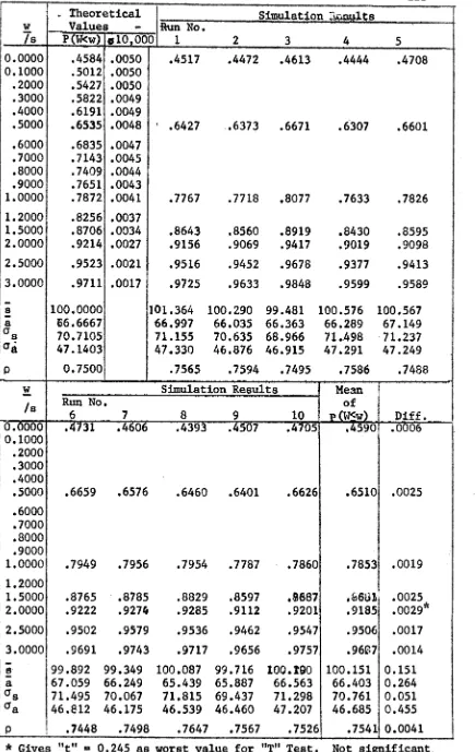
12. In Section 15 we compute the theoretical result for the queue for a mean load per server (p) of 0.75 and compare this with the pooled and individual results of ten independent computor simulation runs each with 10,000 arrivals.

The result of this comparison is quite pleasing. Apparently this analytic method works.

13. In Section 16 we show why the random walk of the GI/G/2 queue gives rise to Laplace Transformations which have singularities with rather interesting loci and interpret this result probabilistically by showing that the traditional notion of first come first served queue operation is strictly equivalent to what we there call "Queuelet Operation” .

This Section ends with some suggestions and conjectures regarding approximations, starting approximations and possible bounds.

14. Section 17 presents somewhat abbreviated proofs of Theorems which suggest that the functional and integral equations for

1

Glossary of Notation

This section contains the definitions of the main notation used in this thesis.

1.1 LCTjt] Symbols

til a is the time interval between the arrival of the (n-1)

n

customer and that of the nth.

A(a) is the probability that any interarrival interval is less than or equal to a.

a is the mean interarrival time,

n^, is a general coefficient in the bivariate power series f(z^,Z2) discussed in paragraph (5.1.5).

a ,... is a generalization of a. , used in the definition

to«* in ti- 11m

I n 1 2

of a multivariate analytic function.

X^**^ is a point in m dimensional complex space. It is the such point and is a centre point of the

element of a continuation process which also defines a Singular Chain.

Am(*) used to indicate the Amplitude of the variable placed within the parenthesis.

B(s) is the probability distribution for the customer service times. That is B(s) ■ P(S < s)

Complex space in n dimensions. See also which is the equivalent Euclidean 2n dimensional space.

2

CKl(4 »6) whence (^(<{>,0), CR 1 4,0), CK2(<|>,0) etc. for which see Section 8, are variants on 0(0,0) wherein the numbers K and L of the E^/E^/2 queue appear explicitly.

C^(w) for 0,1,...L-l is the function defined by the th

substitution of the l branch out of L branches of f(w) in the relationship:

C(f (go) ,u>-f (w)) * M(f (w) ,a)-f (w))

Also written as for 0,1,...,L-l for short. C (to) A column vector formed from the C (w) for all

A 1

1 *» 0,1,...,L-l. See equation (11.7.4).

0(0,0) A complex valued function of the complex variable defined by equation (13.13.5).

«^denotes a domain. Domains are defined by Definition (5.5.1.). D(z°,r) denotes a polydisc in multidimensional complex space.

Polydisc is defined by Definition (5.1.6).

D £ denotes an elementary disu of the D(z°,r) class such that all radii r<e where £ is arbitrarily small. See Definition

(5.1.7) where this is used.

d is used to locate a common discontinuity of A(a) and B(s). See discussion after equation (6.3.4).

3f__

denotes the primary domain of analyticity of the Laplace Transformation X_ (4>, 9) in the bivariate complex space of

4> and 6

Df

similar

to ^ f

but relates to X ($>0)* See Lemma (6.11).

3

Dq denotes differentiation with respect to 0

z. See proof of Lemma (6.21) and Section 7.

D(4>,0) denotes a complex valued function of the complex variables $ and 0. See equation (9.3.1) et seq.

d ^ ( 0 ) denotes for each m = 0,1,...,K an analytic function of all finite 0 s.t. Re(0)>O. See Theorem (9.3.3).

til til

d^_. denotes the j of the m set of complex valued coef­ ficients in a power series representation of D($,0). See equation (9.3.21).

d (0) denotes for each m « 0,1,...,K the d ^ ( 8 ) defined above after we have shown these to be analytic for all finite 0. See equation (9.6.18).

E^n denotes 2n dimensional Euclidean space.

Ev denotes an Erlang distribution with K exponential stages. K.

2

That is a Gamma (or Pearson III) or a X distribution with 2K degrees of freedom.

E^ denotes a similar distribution with L exponential phases. E denotes a real variable used in the proof of Lemma (6.5(i)).

See Result 1 and equations (6.5.1.1) and (6.5.1.A). E also denotes a real variable used in the proof of Lemma

(6.5).

4

E(0) denotes a complex valued function of 0 used in the proof of Theorem (9.3.2). See equation (9.3.9).

e and jt.Except where confusion might arise e is used to denotes the base of the Naperian logarithms. However where e is also used as a real variable the symbol

Z

is

substituted as the Naperian base.

Note; Originally it was intended to use

Z

as the Naperian base throughout to avoid any confusion. However a problem arose and this would now necessitate extensive retyping. e denotes a real variable used in the proof of Lemma (6.5(i)). e denotes a real variable in the proof of Lemma (6.5).

e ^ denotes a real variable at the moment just after the n arrival at the queue. See proof of Lemma (6.5). e v denotes a real variable at the moment just before the

til

n arrival at the queue. See proof of Lemma (6.5). F(w) denotes Probability {W<w)where W is the waiting time

of an arbitrary customer.

f(z^yZ^)

denotes a complex valued analytic function of the complex variables z^ and z^. See Definition (5.1.5). f(z^,...,zn) denotes the complex valued analytic function of

n complex variables z^, z?p...,z .

F anf f denote real variables used in R(f) * Prob {F<f} in the proof of Lemma (6.5).

5

f^Cw) denotes for m = 0,1,...,L, the m of a set of poly­ nomials in w which arise when C(v-y,y+w-v) is written down succinctly.

? L (co) denotes a polynomial in g o, related to f^(w) by the equation (A-00) ?L (co) * fL (co) which can be shown to hold for any integral K and L. See Sections 12 and 13. G(v^,V2) denotes the joint probability distribution of the

variables v^ and v^.

til

g_j(oo) denotes for j = l,2,...,m the j of m entire functions of u).

denotes a real variable used in the proof of Lemma (6.5). See equation (6.5.1.19).

g denotes a real variable used to define Prob {G<g} in proof of Lemma (6.5).

G denotes a real variable used in the statement and proof of Result 2 employed to prove Lemma (6.5).

*1 ^

G^ (co) denotes: D zJ { ^ ( z - y j y + w - z ) ^

G (to) denotes a column vector of the G (to) for j = 0,1,...,L-l

X J

See equation (11.7.4).

H(j) denotes for j * 0,1,2,.. the set of limits Lim { P ^ x ^ z n G y + t o - z ) ^

Re (to)**»

6

h^(co) denotes for i * 1,2 two rational functions of w used to define the solution of the E /M/2 queue.

H^Gi}) denotes for i * 1,2 two polynomials in w used to

define the functions G^(o)) and G^Co)) used in the solution of the queue.

h denotes the mean service time s for the M/M/2 queue in order to be consistent with A.K. Erlang's notation. Im (•) denotes Imaginary Part of ,

I(0,0Q ) denotes a Laplace-Stieltjes (L.S.) integral E(£, ^ 6° )y ®°y ) with respect to a distribution F(y) where 0q is an arbitrarily chosen centre point

s.t. Re(0^)>O. See proof of Theorem (5.3.3).

I_(4>,0) denotes a L.S. integral with respect to the set function

x_(x>y)

used in the proof of Lemma (6.12). I+ (-U,y+w) denotes a L.S. integral with respect to the distribution X+(x >y) defined by equation (6.16.3).

denotes a L.S. integral used in the proof of Theorem (5.3.2).

denotes a L.S. integral over a bivariate Carterian space with respect to a measuret/i£ (dxXdy) .

j ( z^ t..., z^) denotes the n dimensional generalization of

(<M).

i d e n o te s a g e n e r a l i n t e g e r v a r i a b l e u se d a s an in d e x .

A lso u s e d to d e n o te / - T and t h e u n i t o f im a g in a r i e s

w here t h i s i s n e c e s s a r y and no c o n f u s io n w i l l a r i s e .

A lso u s e d a s a s u b s c r i p t .

j d e n o te s a g e n e r a l in d e x .

j Q(a)), j 2 d e n o te t h r e e r a t i o n a l f u n c t i o n s o f to.

See S e c tio n 13 and e q u a t io n ( 1 3 . 8 . 6 ) ,

J + (6 ) d e n o te s a L a p la c e I n t e g r a l . F i r s t u se d i n t h e p r o o f

o f Lemma ( 6 . 3 ) .

J__(<{>,9) d e n o te s a L a p la c e I n t e g r a l ta k e n o v e r t h e r e g io n

s . t . x e (-o ° ,0 ) and y e ( - ° ° ,0 ] . See p r o o f o f Lemma ( 6 . 6 ) .

__(4),6) d e n o te s a s i m i l a r L a p la c e I n t e g r a l w here th e s e t

f u n c t i o n i s ^n \ _ ( x , y ) r a t h e r th a n x ( x , y ) .

J _ ( 0 ) d e n o te s a L a p la c e I n t e g r a l o v e r t h e r e g io n su ch t h a t

x e ( - ° ° ,0 ) y e ( - 00 , 00) i f Re (4))->-“ .

J d e n o te s th e f i r s t o f L r o o t s o f u n i t y . Thus' d e n o te s

th e 1 ^ su ch r o o t .

^10* ^11* ^12 ^ e n o te t ^ie t h r e e c o e f f i c i e n t s o f t h e p o ly n o m ia l

H^(co). See e q u a tio n ( 1 3 . 0 . 2 ) .

K d e n o te s t h e number o f e x p o n e n t ia l s t a g e s i n an E r la n g K,

d i s t r i b u t i o n .

1 i s an in d e x w hich i d e n t i f i e s th e r o o t o u t o f L r o o t s 9

3

L denotes the number of exponential stages in an Erlang L, distribution.

and l ^ ^ denote the maximum and second maximum of the set of departure times for all customers entering the queueing system before the nt^1.

t/C(dx,dy) denotes a measure defined for all subsets of a bivariate Cartesian product set.

denotes an L by L square matrix of functions of

which are the coefficients of the (oj) for 1 * 0,1,..., L-l. See Section 11.

(go) denotes the out of L, functions used in Section 11. M($,0) denotes a bivariate function defined by equations

(7.19) and (7.20).

F?(6) denotes a function used as an upper bound in the proof of Theorem (9.3).

m denotes a general index variable as in dm (0). Also used to denote a measure.

m (co) denotes a Laplace Transformation of the measure m with respect to to.

(n) * *

m (w) denotes the m (w) which may be defined immediately before the n ^ arrival at the queue.

m(<}>) denotes a part of the limit defined by equation (9.7.38). n denotes an index variable generally associated with stages or

til

9

n! denotes factorial n. n is now used as an index unrelated to the number of arrivals at the queue.

P(*) generally denotes the probability of the event or condition within the parentheses.

and denote probabilities of there having been m arrivals since the queue was last empty for two different terminal conditions.

P(y/x) denotes Prob{Y<y given x}

^ d e n o t e s an elementary disc centred on the point which punctures the complex plane in w.

P(0), P(l) and P(2) respectively denote the probabilities of emptyness (no servers busy), one server busy and two servers busy for the two server queue.

p denotes a general complex variable used in Section 4. Also used as a probability.

p(j/x) denotes the conditional probability of j stages for j = 1,2,...,L when given x.

Q(e) denotes Prob {E<e} for ee[0,°°) A

Q (0) denotes the L.T.w.r. to 0 of Q(e).

Q(e) denotes a probability distribution for eeC-00,00).

A

Q (0) denotes the L.T. of Q(e).

£ ^

10

Q(£/x) denotes the conditional distribution of £ given x til

at the moment just before the n arrival.

(n)Q^(0) and (n)Q^(0) denote the L.T’s of (n)Q(e/x) and ^n ^Q(e/x) with respect to 0 respectively.

q(jjCj)) denotes:

00

- f p(j/x)e ^dlK x ) 0+

q denotes a real constant.

Re(*) denotes the real part of the variable in the parentheses. til

denotes the radius of convergance of the n element of a continuation chain in univariate complex space. Also used to denote n dimensional real space.

denotes the jth radius of convergance for j ■ 1,2,... n til

for the n element of a continuation chain in n dimensional complex space,

denotes a region. R denotes a real number.

ft, denotes the portion of boundary included in

R(f) denotes the probability distribution Prob {F<f). R (0) denotes the L.T. of R(f).

and denote the respective first regions where the & &

L.T's X (0,9) and X_+ (0»®) are continuous.

11

R^ and denote r-j+r2 an^ r]_r 2 resPect:Lvely• Used in the solution of E /E0/2.

K Z

denotes for i * 1,2,...,L a set of complex numbers which locate singularities. Also used as r_j to indicate the radius of a polydisc.

til

S denotes the service time of the n customer to arrive, n

$u denotes a singular chain in univariate complex space. denotes a singular chain in multivariate complex space. denotes a two dimensional set.

^ d e n o t e s the two dimensional support set for ^n 'x+ (x >y)

0 0 0 0

Sg, S^, S2 and are a set of four constants used in the &

definition of x+ ($»0) for the queue, s denotes the mean service time.

9 denotes a constant used in the definition of the x. ($>0) of the E^/M/2 queue.

til

t denotes the absolute time at which the n customer n

starts service.

T(g) denotes an arbitrary probability distribution Prob {G<g} for all gefo,00)

Note: t and T are also used in specific references to Students "T" Test in Section 15.

u denotes the sum x +v • See Section 2.

n n J n

12

V x are a set of variables analagous to the

and V2^n ^ of the two server queue which describe the delay state of the C server queue at the moment just before the n th arrival.

v denotes a complex variable. Generally used as in equation

(

11

.

2

).

W denotes a waiting time.

denotes the waiting time of the n ^ customer.

denotes the waiting (or since the server became free if < 0) til

time for the n customer at the GI/G/1 queue. W(f,g) denotes a bivariate probability distribution. W (6) denotes the L.T. E(£ 0{max(0,F G)}^ reSpect to

W(f,g).

Xn one of two real variables used to describe the state til Second Harkov Chain at the moment just before the n arrival.

x denotes a real continuous variable used in the description of the random walk shown in Figure 2.1.

x and x are also real continuous variables used in this

n n

description.

x ^ denotes a real variable used in the description of the Second Markov Process. The (n) refers to the observation of x at the moment just before the n tn arrival.

x (n) denotes a real variable immediately after the ntl1

13

y(ii) denotes a real variable at the moment just before the t h 4 n

n arrival.

y denotes a real variable of the walk shown in Figure 2.1. Also used generally in the description of the probability spaces for the two server queue.

yn and yn are variables similar to y used in the description of the walk shown in Figure 2.1.

z denotes a complex variable. Frequently used in the manner established by equation (7.14).

1.2 Greek Symbols *

« (P) denotes the Laplace Stieltjies Transformation (L.S.T.) of the distribution A(a) with respect to the complex variable p.

5 (u) denotes a probability density function such that; a

A (a) =* J “ (u) du 0

* is also used as a general complex variable as in where D refers to differentiation.

it

ß (p) denotes the L.S.T. of the distribution B(s) with respect to the complex variable p.

it

3 (q,4>) denotes the L.S.T. of the distribution B(s) when the integration ceases when s = q and with respect to the complex variable (J>.

14

ß is also used as a general complex variable as in where the D refers to differentiation.

^n \ ( x ) denotes the distribution of where x^n ^e C”00»00) is the real variable of the Lindley (i.e. GI/G/1) walk at

th

the moment just before the n arrival.

denotes a concentration of probability at zero.

(n) *

Y (z) denotes the L.S.T. of y(x ) with respect to the complex variable z and over all xe (-00,00)

^n>Y+(z) denotes the L.S.T. of integrated for all

xe£o,°°)

and w.r.to z.

* (n)

Y_(z) denotes the L.S.T. of Y(x )w *r # t0 z for all xe(-°°,0). ^n ^6+ (z) denotes the sum;

(n)Y > ) + (n)Y > )

which is the L.S.T. of a proper distribution ^ 6 (x) for all xefj),00) .

/ \ ^

;6 (z) denotes the difference;

<n)Y*(z) - (n)Y*(0)

which is the L.S.T. of a bounded set function Y (x) which has zero total variation for all x£(-°°,o] .

* ' *

o \z) andö (z) denote related functions defined by equations

• •

(16.2.5) and (16.1.14) respectively.

i

d

15

n denotes an angle, i.e. an amplitude in the complex plane. 9 denotes a complex variable.

^TTCxjy) denotes the distribution of x and y immediately before the n*"*1 arrival. 7r(x,y) is the ergodic limiting form, if it exists.

^ tt (<J>,0) denotes the L.S.T. of ^Tr(x,y)

denotes the probability that the queue is empty just til

before the n arrival.

is the ergodic limiting value just before an arrival,if this exists.

^Tr^(y) denotes the probability of the event that at the til

moment before the n arrival at the two server queue, one server is free and the other has a residual service time of at most y.

TT^(y) is the ergodic limiting form, if this exists. tt^ (6) denotes the Laplace Transformation of Tr^(y) with

respect to 0.

Tf^Cy) denotes any aggregation of probability inherent in 7r(x,y) which lies on the line y£(0,°°) when x » 0.

tt^ (0) denotes the L.T. of ^ ( y ) .

'n(x) denotes the otherwise unconditional probability that X^n ^<x^n ^ at the moment just before the n ^ arrival, p denotes the mean traffic load per server.

16

a denotes a real constant. Also used to denote the standard deviation of a distribution as say tftojöoo in Section 15.

til

t denotes the absolute time at which the n customer n

leaves the queue.

(j) denotes a vomplex variable.

X+ (x,y)

denotes a distribution at the moment just before

til

the n arrival and with support set such that 0<x<y<o°. X,(x,y) is the ergodic limiting form, if this exists.

*7* (n \

X_(x »y) denotes a bivariate set function over the space . .xe(-°°,0[ ye]*»00)

X_(x,y) is the ergodic limiting form, if this exists. ^n \ + ($,0) denotes the L.S.T. of ^n \*(x,y)

& £

X+ (^,6) denotes the L.S.T. of X+ (x iY)

^ x ($>6) and x ($>9) denote the L.S.T's of ^ x _ ( x >y) and X (x,y) respectively.

^n ^X(x,y) denotes the sum;

^ X + C x j y ) + ^ x _ ( x »y) e (n)iT(x,y) The ergodic limiting form is x(x »y) and; *

X (<J>,0) denotes its L.S.T. which also satisfies X * ( < M ) * X*( < M ) + X*W*6)

^n \ + (V1+ ,V2+*,... ,Vc+ ) is the distribution for the C server queue analagous to ^ X + (x,y).

17

X_(0,0) denotes a portion of x (0,0) obtained by integrating the L.T. of x (x,y) only over the region such that -oo<x<y<0.

it it

X_+ (0,0) denotes the portion of x (0,0) obtained by integrating the L.T. of x (x,y) only over the region such that xe("°°,0] and ye(0,oo) . Thus;

X_(<M) * X*.^90) + x!+(0»0)

(n)X_(0,6)

and

^X_+(0,0)

are analagous L.S.T's of ^ x _ ( x , y )

integrated over the same support sets. (n) (M)

X (x) denotes the marginal distribution of x at the ttl

moment before the n arrival.

X^M) (x) denotes the ergodic limiting form of (x) if this exists.

X+ (0)

denotes

X+ (0»0)

when 6 * 0 and is thus the L.S.T. of the ergodic limiting waiting time distribution for the two server queue.

0(x) denotes a distribution on the positive half line. 0 (0) denotes the L.S.T. of 0(x) with respect to 0.

0 denotes a set of exceptional points where X+ (0>9) Is not bivariate analytic if 0 ■ -y.

w denotes a complex variable.

ß (0,0) denotes a sum of functions for the ergodic queue.

T

See equation (6.4.1)

it

18

(M)

ß+ (x) denotes the marginal distribution of x derived from fi+ (x,y)

(nV

M)

+

(x) denotes the distribution analagous to ß^jp(x)

th

which holds at the moment before the n arrival. X denotes a real constant used to specify the stage rate

for the Er distribution of interarrival times for the

U denotes a real constant which specifies the service rate for each stage of the service time distribution of the EK./El/2 Q u e u e *

1 9

.

2• Two Alternative Markov Processes for GI/G/2.

We here derive the recurrence which defines the basic

embedded vector Marlcov chain for GI/G/2. This result is

similar to but not identical with that quoted by Kiefer

and Wolfowitz (7) and Pollaczek (14, 15). We shall refer

to this as the First Markov Chain and from this derive a Second Markov Chain which defines what Pollaczek calls the sequence of “last ends" which is also used by Kiefer and

Wolfowitz. Both chains define the same distribution

function for the waiting time (w^) experienced by the n ^

arriving customer, but the second leads to a simpler

analysis. We shall also use ordered variables, whereas

Pollaczek does not.

2.1 Assumptions.

We have two servers operating independently and in simple parallel serving a single queue where the customers arrive singly, and are served in the order of their arrival. Successive interarrival intervals are assumed to be

independ-ty

entband identically distributed. The service times o£ the

individual customers are also assumed to be independent of both the individual customer or the server and to be

identically distributed. This is the system considered as

GI/G/2 in the Kendall notation, see [5,6]. til

Let S be the service time of the n customer to

n

arrive. As defined above is independent of both n

t tl

and which of the two servers handles the n customer.

Let t be the absolute time at which the n t^1

n

2 0.

Let

T

be the absolute time at which the

n

n

customer leaves the system.

Thus:

T

* t + S .

n

n

n

Let a

be the time interval between the moment of

n

fc ti th

arrival of the

(n-1) 1

customer and that of the n1

Remark:

There appears to be no mathematical restriction

which would prevent the customer interarrival time

distribution from having a saltus at zero.

Hence "multiple

arrivals"

should be permissible in this very restricted

sense.

We shall not deal with such cases in this thesis.

2.2 Development of the First Markov Process.

This first Markov process uses the method of ancillary

variables to describe strictly

(i.e. exactly)

the state

of the system just before the moments of arrival of the

customers.

The second which may be simply derived from

it

gives exactly the same delay distribution but offers a

simpler analysis since it avoids certain ambiguities.

For

this reason both references (7) and (14) use the second

/

process as shall we.

However, neither (7) nor (14) gives a

derivation of either process.

We therefore give the follow­

ing derivation both for its intrinsic interest and to aid

our understanding of the random walk which derives from the

second process.

This is rather important in view of our

later comments on Pollaczek's work.

til

For two servers the earliest time at which the n

customer can be served if he is already present and waiting

for service is

21

since he can be served as soon as at least one of the two servers becomes free and this happens when the second last of the previous customers to depart leaves the system.

Therefore

n

t^ • max[ £ a^, 2nd m a x { T Q , . . . ] (2.2)

i® 1

n tli

if E. . a. is the time at which the n l customer arrives.

i*l i

till

Remark; By this convention the zero ' customer arrived and

commenced service at t^ * 0,

We now introduce the variables;

L i <n) *

l<2 ^n ^ * second m a x { T ^ >T ^ , . . . , }

and use (2.3) in (2.2) to obtain:

n

t - max{ J a . , L ^ n ^}

n ±ul i 2

Let us now define;

V 2 (n> ’ t 2 <" > ' * "i 1 = 1

I a

n

I -i

i«l

(2.3)

(2.4)

(2.5)

and

2 2 .

Then the

Consider analogy with

Also :

t (n+1) L 1

t*

waiting time of the n customer is:

n

w «= t

- y

a.

n n i-i 1

* max { 0 ,L9 - y a .}

1

i-1 X

® max {0,V2 ^n ^}

» ( v 2 ( n ) }+ .

now the (2.3)

v (n+1)

2

(n+1)

(n+1)th

and (2.A)

(n+1)

L2

(n+1) 1

customer to arrive, we define:

n+1

- I

i-l a

i

n+1

- I

i = 1 a

i

By

m a x { l Q , T ^ , • • • »T ^ }

(2*7)

(2 .8)

(2.9)

max{x0 ,Tl .... Tn - l ,t:n+sn } n

max{T0 ,T1 .... Tn _i*

l

i+wn+Sn }a

i*l

23

Similarly: (n+1)

Second m a x { T * , T . -, {V0 (n)}++S + I a.} (2.11)

H i n-1 z n , - 1

i*l

However equations (2.10) and (2.11) contain the same sequence of terms as equation (2.3) except that a new term has been added namely

{{v ,(tl)}+ + S + la }

2 n 1-1 1

Therefore :

v (n+1) (n+1)

2

~

L2

I

i*= 1

second max{i. ,L« , {V0 }++S + 5] a. } - £ a.

1 2 2 n i-1 1 i-1 1

(2

.

12)

/ _ \

since terms smaller than cannot affect the outcome.

Therefore:

V 2 (n+1) - second max {V 1 (n),V ? (n),{V 2 (n)}++Sn ) - an+1

by use of (2.5)

* second max{V_ {V - ^ }++S } - a

-1 2 n n+1

because (V^(n)}+ > V ,

(2.13)

Similarly we may show that§

V (n+1) - max(V (n),{V (n)}++S } - a

1 1 2 n i (2.14)

2 4

.

are known for any n, expressions (2.13) and (2.14) define a Ma r k o v chain for an(j V 2 ^n + ^ . Thus if this time homogeneous chain has a limiting joint distribution G (v i,v 2 ) for the variable and V 2 {n ^ as n °°,

we may define the limiting distribution for the waiting time b y ;

F (w) * P (W < w)

* F ^v 2^

by w = maxlOjV^) ® (v2 ) +

G ( v 1 * °°»v 2^

if v 2 > 0

- g(V;l = ®,0) ■

if v 2 < 0

(2.15)

Note: Necessary and sufficient conditions for the existence of the limiting joint distribution of and V 2 were first given by Kiefer and Wolfowitz in [7).

2.3 The Second Markov C h a i n .

25

Y (n+1) - m a x { { Y (n)}+ ,{X(n)}++S } ... (2.16)

X (n+1) - m i n { { Y (n)}+ ,{x(n)}++S } - a

n n+1 (2.17)

to define the variables X^n ^ and for all n 0,1,2*... . Clearly these equations define a Markov chain which is very similar to that described by equations (2.13) and (2.14). To see that both define the same distribution function w . the

n £ h

waiting time of the n customer to arrive, we show that: {X (n)>+ E {y ^(n)}+

for all n. Write

(Y (n + 1)}+ - (max{{Y(n)}+ ,{X(n)}++S } - a }+ n n-t* jl {X ( n + D } + = {m i n {{Y (n)}'h,{x(n)}++S } - a . _ } +

from (2.16) and (2.17). Write

{V x <n + 1 >}+

. {raax{V1 (n),{V2 (n)}++ Sn } - an+1>+

{V2 (n+D } + - {min {V1 (n).{V2 (n)}++ S n } - an+1>+

from (2.13) and 2.14). Note that:

2 6

.

We postulate:

{x ( n ) }+ - { v 2 ( n ) }+

{Y <n)}+ = {V1 (n)} +

whence

V 1 ^n) < {Y^n ) }+ If < 0 but V 1 (n^ * { Y ^ } * if V.^11^ > 0,

and show that:

{x<n+l)}+ . {v2(n+l)}+

{Y (n+l)}+ . {v^ }

for all n * 0,1,2,... .

P r o o f : If V x (n) < 0

{ (n+l)}+ ,

{{v ( n ) }+ +s

-a ,_}+ « (Y (n+1) }+

1 2 n n+l

{v2<n+l)}+ _ 0 . {x(n+l)}+

by inspection.

If ' > 0 the expressions also give identical

results and the induction is completed. Therefore

w * max{0,V 0 ^}

n £.

■ max{0,X^n ^ } (2.18)

for all n and both the chains give the same delay distribution

However the second chain defines distributions which

27

,

gather rather more of the probability associated with zero

waiting delay into an aggregation (i.e., a saltus) at the

point X * Y « 0 and this is more convenient because it

enlarges the region of convergence of one of the Laplace

integrals used during the solution of these problems.

Finally we note that since both chains consider the states

of the system at the moments just before the arrival of each

customer w

or in the limit as n

if it exists. w is

the delay actually experienced by the customers.

It is not

therefore say, the Virtual Waiting Time of Takacs.

Remarks:

1.

Although most of the analysis which follows will

be concerned with bivariate Laplace Transformation space, it

will be from time to time useful to consider the bivariate

probability space of the equivalent continuous time random

walk and we note that the recurrences defined by (2.16) and

(2.17) can be interpreted in the following way.

Suppose we have a particle undergoing a random walk in the

half quadrant 0 < x < y < «> and subject to the following rules:

(i)

At time

tR + 0 the particle is projected for the n**1

time from some initial position

(xn ,yn)

horizontally and with

constant velocity in such a manner that if it does not encounter

the "mirror" barrier which is the line y * x it reaches the

^ ^ *V «W

2 8

.

(ii)

If it encounters the mirror at y ■ x i.e.

if

S + x > y

it reflects upwards a distance d • S + x - y

n

n

yn

n

n

n

n

and reaches

(x ,y ) where x * y

and y = S + x .

n n

n

n

' n

n

n

Thus this reflection is equivalent to the exchanging of the

variables x and y by the max, min operations of the

recurrence .

(iii)

The particle leaves the point

(x^jy^) anc* drifts t0

the point xn+i>yn+i w^ere

xn+l

xn

an+l

y +1 ’ yn ' an+l

J

n

provided xn+^ >

(iv)

Should the particle encounter the ’sticky" barrier

which is the line x * 0 it becomes captive and slides down

this line at constant velocity to the point

yn+l ‘ yn - an+l

unless:

(v)

The particle becomes trapped at the point x * y * 0

where it rests motionless until time

t

when the process

repeats.

Aj- ,

I

_fvV

2 9

.

M

' P - ■

•

yr

where the numbers correspond with the stages. Naturally

the queueing recurrence is arrived at by observing this random

walk just once per cycle i.e., at the Instants just before

each successive horizontal projection.

(vi) It will also be observed that if the probability of

the particle ever reaching the "sticky” barrier (or the origin) is very very small this random walk will very nearly follow the rul e;

u + S

n n - 2a

w h e r e ,

u

n x + yn J n

3 0

.

consequences which are touched on in later sections.

2.

Following Lindley [11] we note that equations (2.16) and

(2.17) mean that the joint distribution of Y^n+^

and

is identical with that of the max{

}

and min{

}

of the

right hand sides.

See also Section 4 where this is explored

3 1

.

3. The Analogous Maykov Processes for GI/G/C.

Consider that we now have C servers and define

1,2 , . . . , C are V > V > > V

X “ 2 ** * C where the i

real variables which will obey a recurrence to be defined

below: Now note that

*t * max n

t In

a^ , C max{i^ , , • • • (3.1)

i»l

where there are C servers, by analogy with (2.2).

Therefore we may extend the previous derivation to obtain the following analogous results:

v ^(n+l) _ m a x {V i (n>,?2 ( n ) _{,{Vc (n)}++Sn } - a}

- m ax{V l (n),{Vc (n)}++ Sn } - an+1 (3.2)

(n+1)

2 - second m a x ( V 1 (n) ,V2 (n) ,{Vc (n)}*f+Sn } - an+1

- median{V1 (n) ,V2 (n) ,{Vc (n)}++Sn > - an+1 (3.3)

(n+1)

x - »edian{Vx <?>,Vx (n>,{Vc (n))++ Sn > (3.4)

(n+1)

C “ oln{VC ^ ) -{VC (n)}++Sn } ”an+l (3.5)

This is once again a Markov process which may be altered / _ \

by the replacement of some or all of the variables from 1

to by (V1 (n)}+ etc., to {Vc ^n ^}+ without

altering the distribution of w where,

n (n)

w ■ max(0,V ' }

32

.

although the joint distribution of the to is

quite extensively altered.

Note: The above processes use strictly ordered variables with

whereas Pollaczek's treatment [15] does not use any such fixed

ordering of the variables. The fixed ordering appears to

lead to some simplifications in the analysis, and it is the ordering (or sorting) process which in effect generates the more important singularities.

3 3

.

4.

Laplace Stieltjes Transforms.

To proceed further from equations (2.16) and (2.17) we

define the Bivariate Distribution Function of the variables

(n)

(n)

.

x

, y

to be;

^n^Tr(x,y)s

» P ( X ^ n^ < x , Y ^ n^ < y )

(4.1)

for all n * 1,2,...

and where

-°° < x , y < 00

We now define;

l

q

e~padA(a)

where A(a) * P(A < a)

f00

■ J Qe"*paa (a)da

if the density function a(a)

exists

* a* (p)

(4.2)

Also define;

00

/Qe pSdB(s)

where B(s) * P(S < s)

00

:»/0e pS$(s)ds

if the density function

$(s)

exists

34

.

We now reconsider ' -uations (2.16) and (2.17) namely;

<x ( n ) >+ + S „> an+l (2.16)

{ X (a)}+ + S } - a ..

n n+j. (2.17)

and use the previous definitions to write;

. 0 0 . 0 0

00 00 00

I Jf

e

TT(x,y)

-8max ({y }+ , {x^n ^ }+ +s) - <J>min( {y ^ }+ , { x ^ } +

-(n)i

Mo

e '^+<^ a d B ( s ) d A ( a ) d ^ n ^7r(x,y) (4.4)

directly from (2.16) and (2.17) after noting that B(s) and A(a) are independent of n where;

(n)

f

f -<f>x(n)- 0 y (n) , ( n ) - v ,, ,-v

tt* (4>, 6) »

J

1

e y

d

7r(x,y) (4.5) X * -00 y * x

-is the Laplace Stieltjes Transform of the Bivariate D-istribution Function ^n ^7T(x,y) which may exist only for wholly imaginary 4> and 0. The extension to domains is considered later.

-0

-+ CD

I

*

a

it

*

t=

+

3 6.

Excursus. On the One Server Wiener-Bopf M e t h o d .

The simplification of (4.6) which we ahaLluse may be more readily understood if we reconsider the analytic method often used for the one server queue. In our notation, Lindley's equation* (see [11]) reads;

^(n+1) * max{ 0, (W }+ + S - a -} (4.7) n n+1

but if we define say x^11^ such that -00 < x^n ^ < 00, x^n ^ real for all n * 0,1,2,... we obtain;

x (n+l) . { x (n)}+ + s . (A.8)

n n+1

whence given a complex variable z and noting that the distributions of S and a ,, are for all n ■ 0,1,2,...,

n n+1 * *

just the distributions B(s) and A(a) and thus independent of n, we obtain;

(n+1) , ,-v E<e~ZX ) - (n+1\ * U )

00 00 ‘ 00 r r (n) 1 + i / \ = , J I f e ”z {x } + s -aldA(a)dB(s)d(n)Y(x

x 'n '«-co 0 0

(4.9) where ^n ^y(x ) is the Distribution of x^n ^ and ^n ^Y*(z) is ' .

its bilateral Laplace Stieltjes Transformation with respect to z which may of course only exist for z wholly imaginary.

Thus ;

(n+1)Y*(z) - i l l e'z(s_a)dA(a)dB(s)d<n)y(x) - » o 0

00 00 00 ( n )

+ 1 1 1 e“ 2(x + S 'a)dA(a)dB(s)d(n)Y(x)

0 - 0 0

- ß*(z)a*(-z){/

d (n)Y(x)

+ / e"ZX

d (n)f(x)

(A.10)

37.

Nov consider the ordinary bilateral Stieltjes Transformation of a variable where

We may write;

(n)Y * ( 2) - /

e"zvd (n)Y(v)

(4.11)

— 00

and if we define

(n)Y*(z) -

/ e“zvd (n)Y(v)

(4.12)

—

00

and,

(n)Y*(2)

-we note that

/ e"zvd (n)Y(v)

(4.13)

0-/ d (n)Y(v) - (n)Y?(0)

(4.14)

—

00

Therefore we may use (4.14) in (4.10) -to obtain;

(n+1)Y*(z)

“ ß*(2)a*(-z){(n)Y*(0)

+

(n)Y*(z)>

(4.15)

whence if we define new functions for all n, by;

(n)6*(z) - (n)Y*(z) + (n)Y*(0)

and (4.16)

(n)6*(z) = (n)Y*(z) - <n)Y*(0) we obtain by use of these in (4.15);

(n+1)Y*(z)

= 8*(z)a*(-z)

(n)6*(z)

(4.17)

3 8

.

lim{ (n+ l)6?{2)} , js < 0 . > 0

one obtains;

(l-ß*(s)o*(-z))5*(z) « - 6 * (z) (4.18)

T •*

Equations (4.17) and (4.18) are the standard

"Wiener-Hopf" starting points for the extensions of the domains of analyticity by factorization and continuation arguments and thence the determination of the distributions

^n ^6(w) and 6(v) in the limiting case, but those simple

processes are of no great interest for the moment. The

important concept is the essential uniqueness of the

constant ^n ^y*(0) which results from the operation of

"sweeping up“ all the probability from the negative half

line and placing it in a saltus at w * 0 since this makes

the Laplace Stieltjes Transformation of a proper distribution which will satisfy (4.17) and which thus defines

a ^n ^Y*(z) which satisfies (4.15). The reader might also

refer to the comments of Kingman [9] on this point.

We n o w apply these ideas to equation (4.6) as follows. Define •

-

J

e~'*>SdB (a)

0

QO

e*(4>) * / e ‘(|>SdB(s)

and use these in ?4.6) to obtain;