Identification of a multi-dimensional space-dependent heat source from boundary data

White Rose Research Online URL for this paper: http://eprints.whiterose.ac.uk/121279/

Version: Accepted Version

Article:

Hussein, MS, Lesnic, D, Johansson, BT et al. (1 more author) (2018) Identification of a multi-dimensional space-dependent heat source from boundary data. Applied

Mathematical Modelling, 54. pp. 202-220. ISSN 0307-904X https://doi.org/10.1016/j.apm.2017.09.029

© 2017 Elsevier Inc. This manuscript version is made available under the CC-BY-NC-ND 4.0 license http://creativecommons.org/licenses/by-nc-nd/4.0/

[email protected] https://eprints.whiterose.ac.uk/ Reuse

This article is distributed under the terms of the Creative Commons Attribution-NonCommercial-NoDerivs (CC BY-NC-ND) licence. This licence only allows you to download this work and share it with others as long as you credit the authors, but you can’t change the article in any way or use it commercially. More

information and the full terms of the licence here: https://creativecommons.org/licenses/

Takedown

If you consider content in White Rose Research Online to be in breach of UK law, please notify us by

Accepted Manuscript

Identification of a multi-dimensional space-dependent heat source from boundary data

M.S. Hussein, D. Lesnic, B.T. Johansson, A. Hazanee

PII: S0307-904X(17)30580-2

DOI: 10.1016/j.apm.2017.09.029

Reference: APM 11974

To appear in: Applied Mathematical Modelling

Received date: 18 January 2017 Revised date: 11 September 2017 Accepted date: 13 September 2017

Please cite this article as: M.S. Hussein, D. Lesnic, B.T. Johansson, A. Hazanee, Identification of a multi-dimensional space-dependent heat source from boundary data,Applied Mathematical Modelling

(2017), doi:10.1016/j.apm.2017.09.029

A

CCE

P

T

E

D

M

A

N

U

S

CRIP

T

Highlights

• Multi-dimensional space-dependent sources are reconstructed from boundary data.

• Iterative regularization methods are developed.

A

CCE

P

T

E

D

M

A

N

U

S

CRIP

T

Identification of a multi-dimensional space-dependent

heat source from boundary data

M.S. Hussein1,2_{, D. Lesnic}2,∗_{, B.T. Johansson}3 _{and A. Hazanee}4

1_{Department of Mathematics, College of Science, University of Baghdad, Baghdad, Iraq}

2,∗

Department of Applied Mathematics, University of Leeds, Leeds LS2 9JT, UK

3_{Mathematics, Aston University EAS, Birmingham, B4 7ET, UK}

4_{Department of Mathematics and Computer Science, Faculty of Science and Technology,}

Prince of Songkla University, Pattani Campus, Pattani, 94000, Thailand

E-mails: [email protected], [email protected] (M.S. Hussein), [email protected] (D. Lesnic∗

-corresponding author),

[email protected] (B.T. Johansson), [email protected] (A. Hazanee).

Abstract

We investigate the linear but ill-posed inverse problem of determining a multi-dimensional space-dependent heat source in the parabolic heat equation from Cauchy boundary data. This model is important in practical applications where the distribution of internal sources is to be monitored and controlled with care and accuracy from invasive and non-intrusive boundary measurements only. The mathematical formulation ensures that a solution of the inverse problem is unique but the existence and stability are still issues to be dealt with. Even if a solution exists it is not stable with respect to small noise in the measured boundary data hence the inverse problem is still ill-posed. The Landwe-ber method is developed in order to restore stability through iterative regularization. Furthermore, the conjugate gradient method is also developed in order to speed up the convergence. An alternating direction explicit finite-difference method is employed for discretising the well-posed problems resulting from these iterative procedures. Numerical results in two-dimensions are illustrated and discussed.

Keywords: Heat equation; inverse source problem; iterative regularization

1

Introduction

The inverse problem of determining an unknown space-dependent heat source function in the heat equation has been the point of interest of many recent studies, e.g. [1–9]. In these studies, in addition to being mostly restricted to one-dimensional computations, the supplementary information required to compensate for the lack of knowledge of the space-dependent heat source is a final time upper-base, space-space-dependent internal measurement of the temperature or a time-average of it. However, these measurements are intrusive and may also be difficult to take simultaneously at many space locations at the same fixed specified instant of time. In order to overcome such a situation, one may be able instead to measure non-invasively (the unspecified) boundary data.

The uniqueness of solution of this space-dependent heat source problem was

estab-lished in related theoretical studies by Cannon [10], Yamamoto [11] and Dinh Nho

Hao [12, Subsection 4.3.1]. It is also worth mentioning the extension to two space-dependent additive components heat source identification from Cauchy data investigated theoretically in [13].

A

CCE

P

T

E

D

M

A

N

U

S

CRIP

T

continuously on the input data. Thus, the problem is ill-posed and it is the purpose of this study to develop a stable algorithm for solving the inverse space-dependent source problem with Cauchy data and implement this algorithm numerically in two-dimensions. The plan of the paper is as follows. The two-dimensional inverse space-dependent source problem for the heat equation is formulated in Section 2. The additional boundary measurement is prescribed as an overdetermination condition to ensure the uniqueness of the solution. The Landweber iterative method for solving the linear but ill-posed inverse source problem is described in Section 3. It consists of solving a sequence of direct and adjoint problems until a prescribed stopping criterion is satisfied. In Section 4, an alternating direction explicit finite-difference method is described and numerical results are presented and discussed. In Section 5, the conjugate gradient method is developed in order to speed up the convergence. Section 6 investigates numerically a test example mimicking a point source. Finally, Section 7 presents the conclusions of the paper and possible future work.

2

Mathematical formulation

Let T >0 and Ω be a bounded domain with piecewise sufficiently smooth boundary ∂Ω. Consider the inverse source problem of finding the pair (u(x, t), f(x)) satisfying

ut=∇2u+r(t)f(x), (x, t)∈QT := Ω×(0, T), (1)

u(x,0) = φ(x), x_∈Ω, (2)

u(x, t) = β(x, t) on ∂Ω_×(0, T), (3)

∂nu(x, t) = ν(x, t) on Γ×(0, T), (4)

wherenis the outward unit normal to the boundary∂Ω,r,φ,β andν are given functions and Γ_⊆∂Ω is a subportion of the boundary ∂Ω on which the measurement of the flux is performed. We can interchange (3) and (4) to specify instead

u(x, t) =β(x, t) on Γ_×(0, T), (5)

∂nu(x, t) =ν(x, t) on ∂Ω×(0, T). (6)

Obviously, when Γ = ∂Ω then the Cauchy data (3), (4) and (5), (6) coincide, but of

practical interest is also to analyse the partial Cauchy data information on the subportion

Γ of ∂Ω as well. We mention that instead of the overspecified data (4) or (5) we can

measure the ’upper-base’ final temperature

u(x, T) = g(x), x_∈Ω (7)

but this inverse formulation will not be investigated herein; instead we refer to Wang et al. [8] and the references therein.

The uniqueness of a solution (u(x, t),f(x)) of the inverse problem (1)–(4) when r(t) is a constant function (and taken for simplicity to be ₋1), in which case equation (1) simplifies to

ut=∇2u−f(x), (x, t)∈QT (8)

was established by Cannon [10] using the method of separation of variables. However,

when r(t) is not a constant function (or when r(t) is not analytic in time) the proof of

uniqueness of a solution is more sophisticated, as provided by Yamamoto [11] for the

A

CCE

P

T

E

D

M

A

N

U

S

CRIP

T

Theorem 1. Let Ω = (0,1)_×(0,1), Γ = (0,1)_{× {}0_} and r_∈C1_{[0, T]with r(0)6= 0. Let}

(f1(x, y), u1(x, y, t))and(f2(x, y), u2(x, y, t))be two solutions of the inverse source problem

(1), (2), (5) and (6) which, in terms of the differences f := f1 −f2 and u := u1 −u2,

satisfy

ut =∇2u+r(t)f(x, y), (x, y, t)∈QT, (9)

u(x, y,0) = 0, (x, y)_∈Ω, (10)

∂nu(x, y, t) = 0, (x, y, t)∈∂Ω×(0, T), (11)

u(x,0, t) = 0, (x,0, t)_∈Γ_×(0, T). (12)

Then, if f _∈L2_{(Ω) it follows that f = 0 almost everywhere in Ω.}

Both Cannon [10] and Yamamoto [11] went on and provided conditional stability

estimates for the space-dependent source term in the heat equation in a rectangular domain. However, the admissible sets of sources imposed in those papers are seldom satisfied in practice. Consequently, the inverse problems (1)–(4) or (1), (2), (5), (6) are still ill-posed and small errors in the input data (4) or (5) lead to large errors in the output heat source function f(x). This can easily be realised from the following example, which is a two-dimensional version of the one-dimensional example given in [10].

Example of instability.

Consider the inverse source problem (1)–(4) for Ω = (0,1)_×(0,1), T = 1, r(t) = ₋1, Γ = (0,1)_{× {}0_},β =φ= 0 and

−∂u

∂y(x,0, t) =ν(x,0, t) =−

1₋e−2m2_π2_t

√ mπ

!

sin(mπx), (x, t)_∈(0,1)_×(0,1), (13)

where m _∈ N∗

. With this data one can easily check (by direct substitution for example) that the exact solution of the problem (1)–(4) is given by

fm(x, y) = 2√msin(mπx) sin(mπy), (14)

um(x, y, t) =

1₋e−2m2_π2_t

m3/2_π2

!

sin(mπx) sin(mπy). (15)

It can be seen that, as m_{→ ∞}, the input flux data (13) tends to zero, whilst the source function (14) becomes unbounded.

Clearly, in order to restore stability a regularization procedure should be employed and in Section 3 we describe the Landweber method for solving the inverse problems (1)–(4) and (1), (2), (5), (6).

2.1

Direct problem

A

CCE

P

T

E

D

M

A

N

U

S

CRIP

T

For example, using standard notation, the problem (1)–(3) has a unique solution u _∈

L2_{(0, T;H}2_{(Ω)), u}

t ∈ L2(0, T;L2(Ω)), provided that r ∈ C1[0, T], f ∈ L2(Ω), β ∈ L2_{(0, T;H}3/2_{(∂Ω))∩H}3/4_{(0, T;L}2_{(∂Ω)),φ ∈H}1_{(Ω) with compatibility conditionβ(x,0) =}

φ(x) for x_∈ ∂Ω. This is shown, for example, in Theorem 9.1, Chapter IV of [14]; note though that an alternative notation is used there with, for example, W2,1_(Q

T) meaning

L2_{(0, T;H}2_(Ω))∩H1_{(0, T;L}2_(Ω)).

For an elementu_∈L2_{(0, T;H}2_(Ω)),u

t∈L2(0, T;L2(Ω)), by solving the problem (1)–

(3) the restriction of the normal derivative of this solution on Γ_×(0, T) is well-defined and belongs to L2_{(0, T;H}1/2_(Γ))∩H1/4_{(0, T;L}2_{(Γ)), see, for example, Lemma 3.4 in Chapter}

II of [14]. In particular,∂nu|Γ×(0,T)∈L2(Γ×(0, T)).

From a practical viewpoint, it might be preferable to only measure function values of the initial state φ without having any constraints on the smoothness of derivatives, that is, to have φ_∈L2_{(Ω) rather than φ∈H}1_{(Ω). This can be achieved, for example, by}

adding some additional smoothness onr(t) and having a homogeneous boundary condition (β = 0), then the above Dirichlet problem has a unique solution in the above space, with additionally u_∈C1_{(0, T;H}2_{(Ω)) for a givenφ ∈L}2_{(Ω), see Corollary 2.8 in Chapter 7 of}

[15]. Similar conditions can also be specified for the Neumann (direct) problem, when f

is known, given by equations (1), (2) and (6).

For the sake of completeness, we mention that the space L2_{(0, T;X), where X is a}

Hilbert space, consists of measurable functionsu(_·, t) : (0, T)_→X withRT

0 ku(·, t)k2Xdt <

∞. ByCk_{([0, T];X) is understood functionsu such that the mappingu(·, t) : [0, T]→X}

possesses continuous and bounded (in the usual norm) derivatives of order up to k _≥ 0. The space Hk_{(Ω), k ≥0 is the standard Sobolev space of function having (weak) square}

integrable derivatives up to order k, with trace spaceHk−1/2_(∂Ω).

3

Inverse problem

In the inverse problem, we assume that the space-dependent source component f(x) in the heat equation (1) is unknown.

Throughout this section we assume thatr_∈C1_{[0, T],r(0)6= 0 such that, according to}

Theorem 1, a solution to the inverse heat source problem (1), (2), (5) and (6) (or (1)–(4)) is unique.

For the Dirichlet inverse problem (1)–(4) we minimize the functional JDN :L2(Ω) → L2_{(Γ×(0, T)),}

JDN(f) :=

1 2

Kf−ν

2

L2_(Γ×(0,T)), (16)

whilst for the Neumann inverse problem (1), (2), (5) and (6) we minimize the functional

JN D :L2(Ω)→L2(Γ×(0, T)),

JN D(f) :=

1 2

Kf˜ −β

2

L2_(Γ×(0,T)), (17)

where K and ˜K are operators which will be defined below.

A

CCE

P

T

E

D

M

A

N

U

S

CRIP

T

Consider first the inverse problem (1)–(4). Introduce the operator K : L2_{(Ω) →}

L2_{(Γ×(0, T))}

Kf =∂nu¯|Γ×(0,T), (18)

where ¯u solves the direct well-posed problem

  

 

¯

ut=∇2u¯+r(t)f(x), (x, t)∈QT,

¯

u(x,0) = 0, x_∈Ω,

¯

u(x, t) = 0, (x, t)_∈∂Ω_×(0, T).

(19)

The operatorK is linear and injective (due to the uniqueness of the inverse source problem,

[10, 11]). Further, introduce the adjoint problem

    

   

vt =−∇2v in QT, v(x, T) = 0, x_∈Ω,

v(x, t) = 0, (x, t)_∈Γc_×(0, T), v(x, t) =ξ(x, t), (x, t)_∈Γ_×(0, T),

(20)

where Γc_{:=∂Ω\Γ and ξ is a function to be specified.}

Multiplying the first equation in (19) and (20) byv and ¯u, respectively, and employing Green’s formula we obtain (using that ¯u_|t=0 =v|t=T = 0, ¯u|∂Ω×(0,T) = 0, v|Γc×(0,T) = 0)

Z

QT

r(t)f(x)v(x, t)dxdt =

Z

QT

(¯ut− ∇2u)v dxdt+

Z

QT

(vt+∇2v)¯u dxdt

= ₋

Z

Γ×(0,T)

v∂nu ds.¯ (21)

Now, using the definition (18) of the operatorK together with the specifiedv

Γ×(0,T) =ξ, expression (21) can be rewritten as

(Kf, ξ)L2_(Γ×(0,T)) = (f, K∗ξ)L2_(Ω), (22)

where the adjoint operator K∗

:L2_{(Γ×(0, T))→L}2_{(Ω) is defined by}

K∗ ξ=₋

Z T

0

r(t)v(_·, t)dt, _∀ξ_∈L2(Γ_×(0, T)), (23)

where v solves the adjoint well-posed problem (20).

Finally, denote by ˜u the solution of the direct problem (1)–(3) withf = 0, namely

  

 

˜

ut =∇2u,˜ in QT,

˜

u(x,0) =φ(x), in Ω,

˜

u(x, t) =β(x, t), (x, t)_∈∂Ω_×(0, T).

(24)

One can easily observe that the inverse problem (1)–(4) recasts into solving the linear operational equation

Kf =ν₋∂nu˜

Γ×(0,T) =:ν. (25)

A

CCE

P

T

E

D

M

A

N

U

S

CRIP

T

Step 1. Make an arbitrary initial guess f0 ∈L2(Ω) for the sourcef and solve the direct

well-posed problem given by the equations (1) with f =f0, (2) and (3) and denote

this solution by u0.

Step 2. Assume that fk and uk have been found. Let vk solve the well-posed adjoint

problem given by the system of equations (20) with

ξ(x, t) :=ξk(x, t) = ∂nuk(x, t)−ν(x, t), (x, t)∈Γ×(0, T). (26)

Step 3. Put

fk+1(x) = fk(x) +γ

Z T

0

r(t)vk(x, t)dt, x∈Ω, (27)

where γ > 0 is a relaxation parameter to be prescribed, and let uk+1 solve the

well-posed direct problem given by equations (1) with f =fk+1, (2) and (3).

Step 4. Repeat Steps 2 and 3 until a desired level of accuracy has been achieved (for

exact data). For noisy data, use the discrepancy principle to stop the iterations at an appropriate threshold. For more details on the convergence and regularizing character of the Landweber method, see [16].

The inverse problem (1), (2), (5) and (6) is handled similarly by changing the Dirichlet boundary conditions in the direct and adjoint problems (19) and (20) into Neumann boundary conditions. The operator ˜K is then defined as ˜Kf =u_|Γ×(0,T) and we replace expression (26) by

ξ(x, t) := ξk(x, t) =uk(x, t)−β(x, t), (x, t)∈Γ×(0, T). (28)

The adjoint operator is defined as

˜

K∗ ξ=

Z T

0

r(t)v(x, t)dt, (29)

and the plus sign in (27) is changed to minus.

4

Numerical discretisation

The one-dimensional case has been discussed in detail elsewhere, [17, 18], and therefore it will not be considered herein. The two-dimensional case when Ω is a bounded planar domain reflects more the typical properties of the general inverse and ill-posed source problem. For the simplicity of explanation, in the remaining part of the paper we assume that Ω is rectangle and, in fact, we take Ω to be the unit square (0,1)_×(0,1), [10, 11]. Then, to discretise equation (1) in the unit square domain Ω = (0,1)_×(0,1),

ut =uxx+uyy+r(t)f(x, y, t), (x, y, t)∈QT = Ω×(0, T) = (0,1)×(0,1)×(0, T), (30)

we subdivide QT into Mx, My and N subintervals of equal step lengths ∆x = 1/Mx

and ∆y = 1/My, and uniform time step ∆t = T /N. At the grid nodes (xi, yj, tk) given

A

CCE

P

T

E

D

M

A

N

U

S

CRIP

T

4.1

Alternating direction explicit method (ADEM)

Based on the method described in [19], in this section an unconditionally stable numerical procedure for solving the heat equation (30) with initial and boundary conditions (2) and (3) will be outlined.

Let ˜uk

i,j and ˜vki,j be the solutions of the following equations which are multilevel

finite-difference discretisations of (30):

˜

uk_i,j+1₋u˜k i,j

∆t =

˜

uk

i+1,j−u˜ki,j −u˜i,jk+1+1+ ˜uki−+11,j

(∆x)2 +

˜

uk

i,j+1−u˜ki,j −u˜i,jk+1+ ˜uki,j+1−1

(∆y)2 +rkfi,j,

i= 1, Mx−1, j = 1, My −1, k = 0, N , (31)

˜

v_i,jk+1₋˜vk i,j

∆t =

˜

v_ik₊₁+1_,j−˜v_i,jk+1₋˜vk

i,j + ˜vki−1,j

(∆x)2 +

˜

v_i,jk+1₊₁₋˜v_i,jk+1₋˜vk

i,j + ˜vki,j−1

(∆y)2 +rkfi,j,

i=Mx−1,1, j =My−1,1, k = 0, N . (32)

We approximate uk_i,j+1 as the arithmetic mean of ˜uk_i,j+1 and ˜vk_i,j+1, namely,

uk_i,j+1 = u˜

k+1

i,j + ˜vki,j+1

2 . (33)

Rearranging the terms in (31) and (32), we obtain the explicit calculations of ˜uki,j and ˜vki,j:

˜

uk_i,j+1 =au˜k_i,j+b(˜uk_i−+11,j+ ˜uik+1,j) +c(˜ui,jk+1−1+ ˜uki,j+1)

+ ∆t

1 +λrkfi,j, i= 1, Mx−1, j = 1, My−1, k = 0, N , (34)

˜

v_i,jk+1 =a˜v_i,jk +b(˜v_ik−1,j+ ˜vik+1+1,j) +c(˜vi,jk −1 + ˜vki,j+1+1)

+ ∆t

1 +λrkfi,j, i=Mx−1,1, j =My −1,1, k = 0, N . (35)

where

a=

1₋∆t

1 (∆x)2 +

1 (∆y)2

1 + ∆t

1 (∆x)2 +

1 (∆y)2

= 1−λ

1 +λ,

b= ∆t (∆x)2

(1 +λ), c= ∆t

(∆y)2

(1 +λ), λ= ∆t

1 (∆x)2 +

1 (∆y)2

.

The initial and boundary conditions (2) and (3) in discretised form are

u0_i,j =φi,j, i= 0, Mx, j = 0, My, (36)

uk_0,j =β₀k_,j, uk_Mx,j =β_Mk_x,j, j = 0, My, uki,0 =βi,k0, uki,My =β

k

i,My, i= 0, Mx, k= 1, N , (37)

where φi,j = φ(xi, yj), β0k,j = β(0, yj, tk), βMkx,j = β(1, yj, tk), β

k

i,0 = β(xj,0, tk) and βk

i,My =β(xj,1, tk) for i= 0, Mx, j = 0, My,k = 1, N.

From (34), ˜uk_i,j+1 can be computed explicitly. In this case, calculations proceed from the grid point close to the boundaries x = 0 and y = 0, as i, j increase. The needed values such as ˜uk_i−+11,j, ˜uki,j and ˜uki+1,j will be known from the initial and boundary conditions

A

CCE

P

T

E

D

M

A

N

U

S

CRIP

T

(33) to obtain the solution uk+1

i,j .

This procedure is unconditionally stable, as both equations (34) and (35) are uncon-ditionally stable, but the time increment ∆t cannot be taken indefinitely large. It has been noticed in [19] that if the time increment is taken very large, the solution obtained will be stable but may not describe the actual and physical problem. This behavior is common to all unconditionally stable explicit or semi-implicit methods.

When the Neumann flux boundary condition (6) is given instead of the Dirichlet boundary condition (3), then we approximate it as

                          

ν₀k_,j = 4u

k

1,j−uk2,j−3uk0,j

2∆x , j = 1, My−1, k= 1, N ,

ν_Mk_x,j = 4u

k

Mx−1,j−u

k

Mx−2,j−3u

k Mx,j

−2∆x , j = 1, My−1, k= 1, N ,

νi,k0 =

4uk

i,1−uki,2−3uki,0

2∆y , i= 1, Mx−1, k = 1, N ,

ν_i,Mk _y = 4u

k

i,My−1−uki,My−2−3uki,My

−2∆y , i= 1, Mx−1, k = 1, N .

(38)

4.2

Numerical solution of the inverse problem

We aim to obtain stable reconstructions for the heat source f(x, y) together with the temperature u(x, y, t) satisfying the equations (2)–(4) and (30) for the Dirichlet problem or, equations (2), (5), (6) and (30) for the Neumann problem. To assess the accuracy of the numerical solution for the heat source we define the root mean square error by:

rmse(f) =

"

1

(Mx−1)(My −1) Mx−1

X

i=1

My−1

X

j=1

fnumerical(xi, yj)−fexact(xi, yj)

2 #1/2

. (39)

The space grid meshing of the unit square Ω = (0,1)_×(0,1) is kept fixed atMx =My =

10 throughout the computations. The integral involved in (27) is simply approximated by the point rule

Z T

0

r(t)vk(x, y, t)dt ≈ T N

N−1

X

i=0

r(ti)vk(x, y, ti), (x, y)∈Ω. (40)

We consider solving the Dirichlet inverse problem (2)–(4) and (30) with the input data given by

r(t) = 1, t_∈(0, T), (41a)

φ(x, y) = 0, (x, y)_∈(0,1)_×(0,1), (41b)

β(x, y, t) = 0, (x, y, t)_∈∂Ω_×(0, T), (41c)

and the heat flux measurement

∂nu(0, y, t) =ν(0, y, t) =−π(e−2tπ

2

A

CCE

P

T

E

D

M

A

N

U

S

CRIP

T

for Γ = _{0_{} ×}(0,1) and T = 1. The analytical solution of this problem is given by

u(x, y, t) = exp(₋2π2t)₋1

sin(πx) sin(πy), (x, y, t)_∈(0,1)_×(0,1)_×(0, T), (43)

and

f(x, y) = ₋2π2sin(πx) sin(πy), (x, y)_∈(0,1)_×(0,1). (44)

As we also need to illustrate the convergence of the least-squares objective function (16), this is numerically discretised, as

JDN(f) =

1

2kKf −νk

2

L2_(Γ×(0,T)) ≈

T

2N(My −1) My−1

X

j=1

N

X

i=1

(ν₀i_,j−ν(0, yj, ti))2. (45)

We take the initial guess f0 _{= 0 for the heat source.}

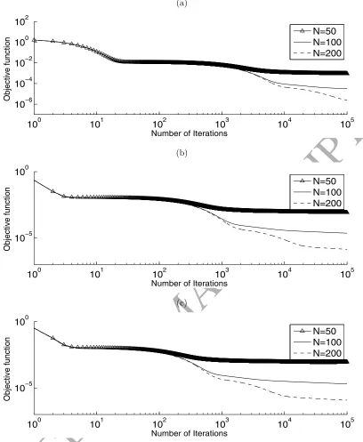
For exact data, i.e. no noise in the heat flux measurement (42), we illustrate in Figure 1 the convergence of the objective function (16), as a function of the number of iterations, for various time grids N _{∈ {}50,100,200_}and various relaxation parametersγ _{∈ {}1,5,10_} in (27). For values of γ greater than about 11 the objective function (16) was found to diverge. This is expected since it is well-known that there exists an upper bound condition

γ < _kK_k−2 _{under which convergence of the Landweber method is assured, [16]. From}

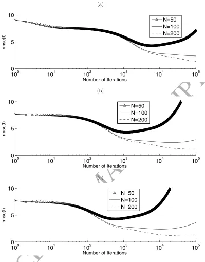
Figure 1 it can be seen that, after about 200 iterations, the objective function significantly decreases as N increases. Also, the rate of convergence increases with increasing γ. The corresponding absolute errors between the numerically retrieved heat source and the exact solution (44) illustrated in Figures 3–5, as well as thermse(f) values calculated from (39) and given in Figure 2 and Table 1 all confirm the convergence and excellent performance of the iterative Landweber method with ADE for solving the inverse Dirichlet heat source

problem for exact data. As shown in Figure 2, the FDM mesh with N = 50 is too

A

CCE

P

T

E

D

M

A

N

U

S

CRIP

T

(a)

100 101 102 103 104 105

10−6 100

10−4 10−2 102

Number of Iterations

Objective function

N=50 N=100 N=200

(b)

100 101 102 103 104 105

10−5 100

Number of Iterations

Objective function

N=50 N=100 N=200

(c)

100 101 102 103 104 105

10−5 100

Number of Iterations

Objective function

N=50 N=100 N=200

Figure 1: The objective function JDN in (16), as a function of the number of iterations, for

A

CCE

P

T

E

D

M

A

N

U

S

CRIP

T

(a)

100 101 102 103 104 105

0 5 10

Number of Iterations

rmse(f)

N=50 N=100 N=200

(b)

100 101 102 103 104 105

0 5 10

Number of Iterations

rmse(f)

N=50 N=100 N=200

(c)

100 101 102 103 104 105

0 5 10

Number of Iterations

rmse(f)

N=50 N=100 N=200

A

CCE

P

T

E

D

M

A

N

U

S

CRIP

T

Figure 3: The numerical solutions and the absolute error between the numerical and the exact solutions, for the heat source with γ = 1, and N = 50, plotted at iteration 6087 which is the minimum point of rmse(f) in Figure 2(a),N = 100 andN = 200.

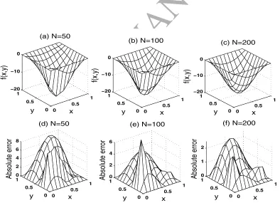
0 0.5 1 0 0.5 1 −20 −10 0 x (a) N=50 y f(x,y) 0 0.5 1 0 0.5 1 0 2 4 6 8 x (d) N=50 y Absolute error 0 0.5 1 0 0.5 1 −20 −10 0 x (b) N=100 y f(x,y) 0 0.5 1 0 0.5 1 0 2 4 6 x (e) N=100 y Absolute error 0 0.5 1 0 0.5 1 −20 −10 0 x (c) N=200 y f(x,y) 0 0.5 1 0 0.5 1 0 1 2 x (f) N=200 y Absolute error

A

CCE

P

T

E

D

M

A

N

U

S

CRIP

T

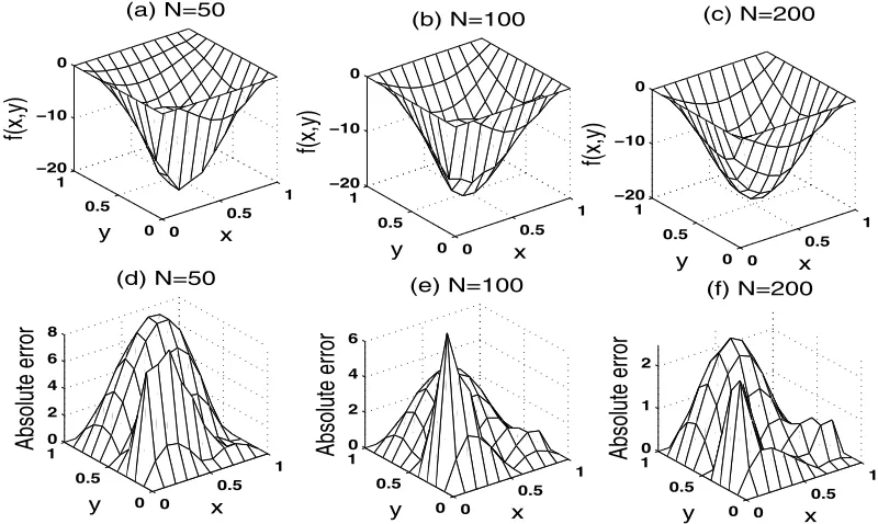
Figure 5: The numerical solutions and the absolute error between the numerical and exact solutions, for the heat source with γ = 10, and N = 50, plotted at iteration 605 which is the minimum point of rmse(f) in Figure 2(c), N = 100, plotted at iteration 10976 which is the minimum point of rmse(f) in Figure 2(c), and N = 200, plotted at iteration 69664 which is the minimum point of rmse(f) in Figure 2(c).

Table 1: The minimum values ofrmse(f) for N _{∈ {}50,100,200,400_}and γ _{∈ {}1,5,10_}.

H H H H H H N γ

1 5 10

50 4.7104 4.7102 4.7099

100 2.6418 2.6403 2.6403

200 1.5091 1.2313 1.2209

400 2.4603 1.5003 1.1313

The computational times to run 105 _{iterations on a laptop machine, with Intel core}

i7 at 2.2 GHz processor and 8 GB of memory are approximately 13, 24 and 42 hours for N _{∈ {}50,100,200_}, respectively. This may imply some slow convergence and high

computational time but then the speeding up can be achieved either by increasing γ or

by using a variable γ (depending on the iterative number k) in (27), as in the conjugate gradient method, [5, 16], described in the next section.

Next we fix N = 100, γ = 10 and consider the case of noisy data (4). This is numer-ically simulated by perturbing the heat flux measurement (42) with Gaussian additive

random noise ǫ with mean zero and standard deviation

σ=p_× max

(y,t)∈(0,1)×(0,T)|

ν(0, y, t)_|, (46)

A

CCE

P

T

E

D

M

A

N

U

S

CRIP

T

We use the MATLAB function normrnd to generate the random variables

ǫ= (ǫj,i)_{i=1,N ,j=1,My}−1, as follows:

ǫ=normrnd(0, σ, My −1, N). (48)

In the case of noisy data (47), we replace ν(0, yj, ti) by νǫ(0, yj, ti) in (16). The total

amount of noise

ε(p) :=_kνǫ₋νexact_k=

v u u t

T N(My −1)

My−1

X

j=1

N

X

i=1

(νnoise_{(0, y}

j, ti)−ν(0, yj, ti))2, (49)

generated from one of these simulations is ε(p) _{∈ {}0.1374,0.2749_} for p _{∈ {}5,10_}%, respectively. This is important to know because in order to obtain a stable solution we need to stop the iterative process described in Section 3 at the first iteration number kd

for which the discrepancy criterion

JDN(fkd)≤τ

ε2_(p)

2 , (50)

where τ is some constant greater than unity, is satisfied, [6, 16].

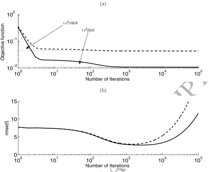
Figures 6(a) and 6(b) show the objective function (16) and thermse(f), respectively, for the first 105 _{iterations for various percentages of noise p ∈ {5,10}%, for τ = 1.3.}

A

CCE

P

T

E

D

M

A

N

U

S

CRIP

T

(a)

100 101 102 103 104 105

10−2 10−1 100

Number of Iterations

Objective function

τε2(5)/2

τε2(10)/2

(b)

100 101 102 103 104 105

0 5 10 15

Number of Iterations

rmse(f)

Figure 6: (a) The objective function (16) and (b) the rmse(f), as functions of the number of iterations, for various noise levels p= 5%(—) andp= 10%(− − −).

According to the discrepancy principle criterion (50), we terminate the iterations of the algorithm at the iteration number kd

kd=

560, for p= 5%,

306, for p= 10%, rmse(fkd) =

3.5659, for p= 5%,

4.5854, for p= 10%. (51)

As expected, aspincreases from 5% to 10% the iterations should be stopped earlier. From Figure 6(b) it can be seen that the objective function (16) decreases as the number of iterations k increases but the rmse(f) starts increasing once

k > kopt =

2618, forp= 5%,

1467, forp= 10%, rmse(fkopt) =

3.0053, forp= 5%,

3.2750, forp= 10%. (52)

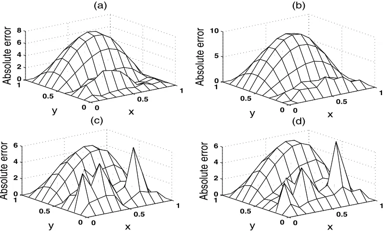
Figures 7(a,b) and 7(c,d) illustrate the absolute errors between the exact solution (44) and the numerically retrieved heat source at the iterations kd and kopt given by (51) and

(52), respectively, for p _{∈ {}5,10_}% noise. From these figures and equations (51) and (52) it can be seen that the accuracy of the numerical solutions improves as the amount

of noise decreases from p = 10% to 5%. Moreover, by comparing Figures 7(a,b) and

7(c,d) it can be seen that although the numerical source solutionf(kopt) is more accurate

than f(kd) it is less stable. This is expected since the Landweber method is a regularizing

A

CCE

P

T

E

D

M

A

N

U

S

CRIP

T

principle (50). Moreover, in practice only kd can be computed askopt uses the knowledge

of the analytical solution which is not available in general.

0

0.5

1 0

0.5 1 0 2 4 6 8

x (a)

y

Absolute error

0

0.5

1 0

0.5 1 0 5 10

x (b)

y

Absolute error

0

0.5

1 0

0.5 1 0 2 4 6

x (c)

y

Absolute error

0

0.5

1 0

0.5 1 0 2 4 6

x (d)

y

Absolute error

Figure 7: The absolute error between the exact (44) and numerical solutions f(kd) for (a)

p = 5% and (b) p = 10% noise. The absolute error between the exact (44) and numerical solutions f(k_opt) for (c) p= 5% and (d) p= 10% noise.

5

The conjugate gradient method

From the previous numerical investigation it was observed that the convergence of the Landweber iterative method described in Section 3 can become prohibitively slow even when the relaxation parameter γ in (27) increases. For example, as previously reported it takes 1 day to run 105 _{iterations for M}

x = My = 10 and N = 100, γ = 10 to achieve

the rmse(f) = 2.6403. In order to speed up the convergence of minimization of the least-squares functional (16) (or (17)) we can improve on the Landweber method and employ instead the regularising γ-free conjugate gradient method (CGM). This iterative algorithm runs as follows.

Let Steps 1 and 2 be the same as in the Landweber algorithm of Section 3. The next steps are as follows:

Step 3 Calculate

dk(x) = −zk(x) +βk−1dk−1(x), k≥0 (53)

with the convention that β−1 = 0 and

βk−1 =

kzkk2_L2_(Ω)

kzk−1k2_L2_(Ω)

, k _≥1, (54)

where the gradient (23) is given by

zk(x) =−

Z T

0

A

CCE

P

T

E

D

M

A

N

U

S

CRIP

T

Step 4 Solve the direct well-posed problem given by the equations (19) with f =dk, to

determine Kdk defined by (18). Set

αk =

kzkk2_L2_(Ω)

kKdkk2_L2_(Γ×(0,T))

, k _≥0, (56)

and pass to the new iteration by letting

fk+1(x) = fk(x) +αkdk(x), k ≥0. (57)

Step 5 This step is the same as Step 4 of the Landweber algorithm of Section 3.

In what follows, we consider the same example as in Section 4. We takeMx =My = 10.

The L2_{(Ω)-norm of the functions involved in (54) and (56) is calculated as}

kz_k2_L2_(Ω) =

1

(Mx−1)(My −1) Mx−1

X

i=1

My−1

X

j=1

z2(xi, yj). (58)

For exact data, Figures 8(a) and 8(b) show the objective function JDN in (16) and

the rmse(f) in (39), respectively, as functions of the number of iterations, for various

N _{∈ {}50,100,200_}. The corresponding absolute errors between the exact solution (44) and the numerical CGM heat source are shown in Figure 9.

The minimum values for rmse(f) are rmse(f) _{∈ {}4.5997,2.5783,1.5583,1.1328_} for

N _{∈ {}50,100,200,400_}, respectively. By comparing these values to those obtained in Table 1 obtained with the Landweber method (compare also Figure 8(a) with Figure 1, Figure 8(b) with Figure 2, and Figure 9 with Figures 3–5) it can be seen that the CGM

gains at least two orders of magnitude speed of convergence, i.e. the CGM uses 103

iterations instead of 105 _{required by the Landweber method to achieve the same level of}

A

CCE

P

T

E

D

M

A

N

U

S

CRIP

T

100 101 102 103

10−6 10−4 10−2 100

Number of Iterations

Objective function

N=50 N=100 N=200

(b)

100 101 102 103

0 5 10

Number of Iterations

rmse(f)

N=50 N=100 N=200

Figure 8: (a) The objective function J_DN in (16) and (b) the rmse(f) in (39), as functions of the number of iterations, for N _{∈ {}50,100,200_}, using the CGM for exact data.

0 0.5 1 0 0.5 1 −20 −10 0 x (a) N=50 y f(x,y) 0 0.5 1 0 0.5 10 2 4 6 8 x (d) N=50 y Absolute error 0 0.5 1 0 0.5 1 −20 −10 0 x (b) N=100 y f(x,y) 0 0.5 1 0 0.5 10 2 4 6 x (e) N=100 y Absolute error 0 0.5 1 0 0.5 10 1 2 3 x (f) N=200 y Absolute error 0 0.5 1 0 0.5 1 −20 −10 0 x (c) N=200 y f(x,y)

Figure 9: The numerical solutions and the absolute error between the numerical and exact solutions, for the heat source with N = 50, plotted at iteration 78 which is the minimum point of rmse(f) in Figure 8(b), N = 100, plotted at iteration 715 which is the minimum point of

rmse(f) in Figure 8(b), andN = 200, using the CGM for exact data.

A

CCE

P

T

E

D

M

A

N

U

S

CRIP

T

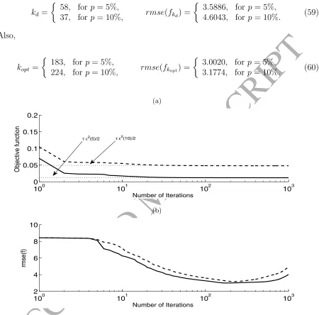
show the objective function (16) and thermse(f), respectively, for the first 103 _iterations

for various percentages of noise p _{∈ {}5,10_}% for τ = 1.3. This yields the thresholds in (50) given by τǫ2₂(p) _{∈ {}0.0123,0.0491_} for p _{∈ {}5,10_}%, respectively. According to the discrepancy principle criterion (50) we cease the CGM iterations at iteration number

kd=

58, for p= 5%,

37, for p= 10%, rmse(fkd) =

3.5886, forp= 5%,

4.6043, forp= 10%. (59)

Also,

kopt =

183, forp= 5%,

224, forp= 10%, rmse(fkopt) =

3.0020, forp= 5%,

3.1774, forp= 10%. (60)

(a)

100 101 102 103

0 0.05 0.1 0.15 0.2

Number of Iterations

Objective function

τε2(5)/2 τε2(10)/2

(b)

100 101 102 103

2 4 6 8 10

Number of Iterations

rmse(f)

A

CCE

P

T

E

D

M

A

N

U

S

CRIP

T

0.5

1

0 0.5 1 0 2 4 6 8

x (a)

y

Absolute error

0

0.5

1

0 0.5 1 0 5 10

x (b)

y

Absolute error

0

0.5

1

0 0.5 1 0 2 4 6

x (c)

y

Absolute error

0

0.5

1

0 0.5 1 0 2 4 6

x (d)

y

Absolute error

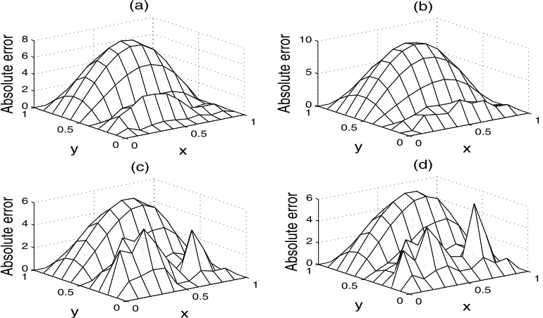
Figure 11: The absolute error between the exact (44) and numerical solutions f(kd) for (a)

p = 5% and (b) p = 10% noise. The absolute error between the exact (44) and numerical solutions f(kopt) for (c) p= 5% and (d) p= 10% noise, using the CGM.

Figure 11 illustrate the numerical solutions for the heat source at the iterations kd

and kopt given by (59) and (60), respectively, for p ∈ {5,10}% noise in comparison with

exact solution (44). Comparing the expressions (51), (52) and Figure 7 obtained using Landweber method with the expressions (59), (60) and Figure 11 and obtained using CGM it can be seen that the same levels of accuracy and stability are achieved by both iterative regularization methods but the CGM is much faster.

6

Another test example mimicking a point source

In the previous sections 4.2 and 5 we have applied the Landweber method and the CGM, respectively, for solving the inverse problem (2)–(4) and (30) with the input data (41a)– (41c) and (42) having the analytical solution (43) for the temperature and (44) for the heat source.

In this example, we consider reconstructing the function

f(x, y) = 1

a2_πexp

−(x−x

0₎2_{+ (y−y}0₎2

a2

, (61)

where (x0_{, y}0_{) = (0.5,0.5) anda= 0.3, mimicking a point source of unit strength/intensity}

located in the middle of the square plate Ω = (0,1)_×(0,1). We also takeT = 1,r(t) =t+1 and the data (2) and (3) given by φ = 0 and β = 0, respectively. As for this data there is no analytical solution available for the temperature u satisfying the Dirichlet direct problem (2), (3) and (30) with f given by (61), the heat flux (4) on Γ = _{0_{} ×}(0,1) is

obtained numerically using the FDM. The numerical results obtained for Mx =My = 10

A

CCE

P

T

E

D

M

A

N

U

S

CRIP

T

0 0.5

1

0 0.5 1 −0.8 −0.6 −0.4 −0.2 0

t (a)

y

ν

(0,y,t)

0 0.5

1

0 0.5 1 −0.8 −0.6 −0.4 −0.2 0

t (b)

y

ν

(0,y,t)

0 0.5

1

0 0.5 1 −0.8 −0.6 −0.4 −0.2 0

t (c)

y

ν

(0,y,t)

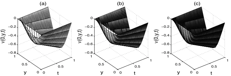
Figure 12: The numerical results for the heat flux ν(0, y, t) =∂nu(0, y, t) obtained by solving

the direct problem with M_x=M_y = 10 and (a) N = 50, (b) N = 100 and (c)N = 200.

From Figure 12 it can be seen that the numerical solution for the heat fluxν(0, y, t) is convergent as the time step decreases. Therefore, we consider the numerically simulated flux from Figure 12(c) at every two time steps as the input data (4) for the inverse problem

(2)–(4) and (30) which is solved with the Mx = My = 10 and N = 100. This way we

avoid committing an inverse crime when numerically simulating the otherwise unavailable input data for the inverse problem. Furthermore, we add p= 1% noise as in (47), where, from (46) and Figure 12, σ= 0.76p. We take the initial guess f0 _{= 0.}

We apply both the Landweber method (with γ = 5) and the CGM with τ = 1.1 in

the criterion (50) giving the stopping iterations

kd =

628, for Landweber,

164, for CGM, rmse(fkd) =

0.4889, for Landweber,

0.4946, for CGM. (62)

Also,

kopt =

6886, for Landweber,

1317, for CGM, rmse(fkopt) =

0.3987, for Landweber,

0.3849, for CGM. (63)

The objective function (45) and thermse(f) error (39), as functions of the number of iterations, are plotted in Figures 13 (a), (b) and 14 (a), (b), and the corresponding numer-ical results obtained afterkopt and kditerations are compared with the analytical solution

(61) in Figures 13 (c), (d) and 14 (c), (d), for the Landweber and CGM, respectively. By comparing these figures it can be seen that the CGM is more efficient as it produces faster numerical reconstructions than the Landweber method with the same accuracy, see also equations (62) and (63). In the meantime, both the Landweber and CGM yield stable solutions, as expected, because of their regularizing character and the employment of the discrepancy stopping criterion (50). Although the error between the numerical and exact

solutions may seem slightly large, there is noise generated both randomly with p = 1%

A

CCE

P

T

E

D

M

A

N

U

S

CRIP

T

100 101 102 103 104

10−5 100

Number of Iterations

Objective function

τε2(1)/2

(b)

100 101 102 103 104 0

0.5 1 1.4

Number of Iterations

rmse(f) (c) 0 0.5 1 0 0.5 1 0 1 2 3 4 x Exact solution y f(x,y) 0 0.5 1 0 0.5 1 0 1 2 3 4 x Numerical solution y f(x,y) 0 0.5 1 0 0.5 1 0 0.5 1 1.5 x y Absolute error (d) 0 0.5 1 0 0.5 1 0 1 2 3 4 x Exact solution y f(x,y) 0 0.5 1 0 0.5 1 0 1 2 3 4 x Numerical solution y f(x,y) 0 0.5 1 0 0.5 1 0 0.5 1 1.5 x y Absolute error

Figure 13: (a) The objective function, (b) the rmse, as functions of the number of iterations, the exact (left), numerical (middle) and the absolute error (right) (c) at the iterationk_opt = 6886 which is the minimum point of rmse(f) and (d) at the iteration kd = 628, for p = 1% noise,

A

CCE

P

T

E

D

M

A

N

U

S

CRIP

T

100 101 102 103 104

10−5 10−4 10−3 10−2

Number of Iterations

Objective function

τε2(1)/2

(b)

100 101 102 103 104 0

0.5 1 1.4

Number of Iterations

rmse(f) (c) 0 0.5 1 0 0.5 1 0 1 2 3 4 x Exact solution y f(x,y) 0 0.5 1 0 0.5 1 0 1 2 3 4 x Numerical solution y f(x,y) 0 0.5 1 0 0.5 1 0 0.5 1 1.5 x y Absolute error (d) 0 0.5 1 0 0.5 1 0 1 2 3 4 x Exact solution y f(x,y) 0 0.5 1 0 0.5 1 0 1 2 3 4 x Numerical solution y f(x,y) 0 0.5 1 0 0.5 1 0 0.5 1 1.5 x y Absolute error

Figure 14: (a) The objective function, (b) the rmse, as functions of the number of iterations, the exact (left), numerical (middle) and the absolute error (right) (c) at the iterationk_opt = 1317 which is the minimum point of rmse(f) and (d) at the iteration kd = 164, for p = 1% noise,

A

CCE

P

T

E

D

M

A

N

U

S

CRIP

T

7

Conclusions

We have presented a computational analysis of the Landweber iterative regularization method for solving the multi-dimensional (with numerical emphasis on the two-dimensional case) inverse heat space-dependent source problem for the heat equation, with Cauchy overprescribed boundary conditions. The Cauchy data is partial in the sense that it is specified only on a small potion Γ of ∂Ω. Thus, the amount of sufficient information to provide the uniqueness of solution is rather minimal and this may be applicable in prac-tical situations concerning limited remote sensing. The CGM has also been developed in order to speed-up the convergence. The direct solver based on ADE finite difference scheme has been employed. Numerical results obtained for both exact and noisy input data show that accurate and stable numerical reconstructions have been achieved. The same conclusions can be obtained for other non-smooth or discontinuous source examples, as shown elsewhere for related inverse source problems, [2, 5, 6].

Future work will consist in extending the analysis and methods of this study to the simultaneous reconstruction of multi-dimensional space-dependent source and diffusivity coefficient, [20].

References

[1] M.N. Ahmadabadi, M. Arab, F. Maalek-Ghaini, The method of fundamental so-lutions for the inverse space-dependent heat source problem, Eng. Anal. Boundary Elements 33 (2009) 1231–1235.

[2] A. Erdem, D. Lesnic, A. Hasanov, Identification of a spacewise dependent heat source, Appl. Math. Model. 37 (2013) 10231–10244.

[3] A. Farcas, D. Lesnic, The boundary-element method for the determination of a heat source dependent on one variable, J. Eng. Math. 54 (2006) 375–388.

[4] A. Hasanov, B. Pekta¸s, A unified approach to identifying an unknown spacewise dependent source in a variable coefficient parabolic equation from final and integral overdeterminations, Appl. Numer. Math. 78 (2014) 49–67.

[5] B.T. Johansson, D. Lesnic, A variational method for identifying a spacewise-dependent heat source, IMA J. Appl. Math. 72 (2007) 748–760.

[6] B.T. Johansson, D. Lesnic, Determination of a spacewise dependent heat source, J. Comput. Appl. Math. 209 (2007) 66–80.

[7] D.D. Trong, P.H. Quan, P.N. Dinh Alain, Determination of a two-dimensional heat source: Uniqueness, regularization and error estimate, J. Comput. Appl. Math. 191 (2006) 50–67.

[8] W. Wang, M. Yamamoto, B. Han, Two-dimensional parabolic inverse source problem with final overdetermination in reproducing kernel space, Chinese Annals of Mathe-matics, Series B, 35B (2014) 469–482.

A

CCE

P

T

E

D

M

A

N

U

S

CRIP

T

[10] J.R. Cannon, Determination of an unknown heat source from overspecified boundary data, SIAM J. Numer. Anal. 5 (1968) 275–286.

[11] M. Yamamoto, Conditional stability in determination of force terms of heat equations in a rectangle, Math. Comput. Model. 18 (1993) 79–88.

[12] Dinh Nho Hao, Methods for Inverse Heat Conduction Problems, Peter Lang, Frank-furt am Main, 1998.

[13] H.W. Engl, O. Scherzer, M. Yamamoto, Uniqueness and stable determination of forcing terms in linear partial differential equations with overspecified boundary data, Inverse Problems 10 (1994) 1253-1276.

[14] O.A. Ladyzenskaja, V.A. Solonnikov, N.N. Uralceva, Linear and Quasi-linear Equa-tions of Parabolic Type, American Mathematical Society, Providence, 1968.

[15] A. Pazy, Semigroups of Linear Operators and Applications to Partial Differential Equations, Springer Science & Business Media, New York, 2012.

[16] H.W. Engl, M. Hanke, A. Neubauer, Regularization of Inverse Problems, Kluwer Academic, Dordrecht, 1996.

[17] A. Hasanov, An inverse source problem with single Dirichlet type measured output data for a linear parabolic equation, Appl. Math. Lett. 24 (2011) 1269–1273.

[18] A. Hasanov, M. Otelbaev, B. Akpayev, Inverse heat conduction problems with bound-ary and final time measured output data, Inverse Problems Sci. Eng. 19 (2011) 985– 1006.

[19] H.Z. Barakat, J.A. Clark, On the solution of the diffusion equations by numerical methods, J. Heat Transfer, 88 (1966) 421–427.