This is a repository copy of
Bayesian model selection for the glacial-interglacial cycle
.
White Rose Research Online URL for this paper:
http://eprints.whiterose.ac.uk/112019/
Version: Accepted Version
Article:
Carson, J., Crucifix, M., Preston, S. et al. (1 more author) (2017) Bayesian model selection
for the glacial-interglacial cycle. Journal of the Royal Statistical Society: Series C. ISSN
0035-9254
https://doi.org/10.1111/rssc.12222
[email protected] https://eprints.whiterose.ac.uk/ Reuse
Unless indicated otherwise, fulltext items are protected by copyright with all rights reserved. The copyright exception in section 29 of the Copyright, Designs and Patents Act 1988 allows the making of a single copy solely for the purpose of non-commercial research or private study within the limits of fair dealing. The publisher or other rights-holder may allow further reproduction and re-use of this version - refer to the White Rose Research Online record for this item. Where records identify the publisher as the copyright holder, users can verify any specific terms of use on the publisher’s website.
Takedown
If you consider content in White Rose Research Online to be in breach of UK law, please notify us by
Bayesian model selection for the glacial-interglacial cycle
Jake Carson†
Department of Mathematics, Imperial College London, UK
Michel Crucifix
Earth and Life Institute, Universit ´e catholique de Louvain, Belgium
Simon Preston
School of Mathematical Sciences, University of Nottingham, UK
Richard D. Wilkinson
School of Mathematics and Statistics, University of Sheffield, UK
Summary.
A prevailing viewpoint in paleoclimate science is that a single paleoclimate record contains insufficient information to discriminate between typical competing explanatory models. Here we show that by us-ing SMC2 (sequential Monte Carlo squared) combined with novel Brownian bridge type proposals for the state trajectories, it is possible to estimate Bayes factors to sufficient accuracy to be able to select between competing models, even with relatively short time series. The results show that Monte Carlo methodology and computer power have now advanced to the point where a full Bayesian analysis for a wide class of conceptual climate models is now possible. The results also highlight a problem with estimating the chronology of the climate record prior to further statistical analysis, a practice which is common in paleoclimate science. Using two datasets based on the same record but with different esti-mated chronologies, results in conflicting conclusions about the importance of the astronomical forcing on the glacial cycle, and about the internal dynamics generating the glacial cycle, even though the dif-ference between the two estimated chronologies is consistent with dating uncertainty. This highlights a need for chronology estimation and other inferential questions to be addressed in a joint statistical procedure.
Keywords: Astronomical Forcing; Glacial Cycles; Model Comparison; Paleoclimate; Sequential Monte Carlo
†Address for correspondence: Jake Carson, Department of Mathematics, South Kensington Campus, Imperial College London, London, SW7 2AZ, UK.
1. Introduction
Throughout the Pleistocene the Earth’s climate has fluctuated between cold periods, in which glaciers
expanded, and warm periods in which the glaciers retreated (Shackleton et al., 1984). The prevailing
theory is that these glacial–interglacial (GIG) cycles are driven, or at least partly controlled, by
variations in the obliquity, precession, and eccentricity of the Earth’s orbit around the Sun, which
affect the distribution of incoming solar radiation (or “insolation”). Obliquity,ε, is the angle between the equator and the orbital plane, and hence affects the distribution of insolation across seasons and
latitudes. Precession is quantified by the angle about the Sun, ϖ, made by the point of perihelion (the point of the orbit when the Earth is closest to the Sun) and the vernal point (which marks the
Spring equinox). At perihelion the Earth is anomalously close to the Sun when compared to a circular
orbit, and so variation in precession affects the seasonal distribution of insolation. Eccentricity, e, measures how much the Earth’s orbit deviates from being circular, and so modulates the effect of
precession.
Milankovitch theory (Milankovitch, 1941) suggests that a positive anomaly of summer insolation
in the Northern Hemisphere prevents the growth of ice sheets, a view supported by experiments with
numerical simulations of the climate system (see Abe-Ouchi et al., 2013, for example). Such positive
anomalies occur when perihelion is near the month of June, and/or when obliquity is anomalously
large. As it is the combination of eccentricity, precession and obliquity that lead to high summer
insolation, there is ambiguity about their respective roles (Crucifix, 2011). Consequently, many
studies have examined the period and magnitude of each in order to see if any one can be considered
to be the primary driver of the glacial-interglacial cycle. Opinion is varied and contradictory, with,
for example, Huybers and Wunsch (2005) arguing for obliquity, Lisiecki (2010) for eccentricity, and
Huybers (2011) for a combination of precession and obliquity. These studies each analysed features of
the insolation signal using significance tests to assess whether the phases of each orbital component are
significantly correlated with estimates of the glacial “termination times” (marking where individual
glacial cycles finish), or whether the insolation signal was anomalously large at termination times.
Differences in the details about how these tests were constructed appear to substantially affect the
conclusions, with different studies finding different orbital characteristics being of primary importance.
It has also been recognised that despite the orbital control, the glacial-interglacial cycle is not
entirely predictable (Imbrie and Imbrie, 1980; Raymo, 1997). This lack of predictability may emerge
from interactions between the astronomical forcing and internal dynamics, in part because the
quasi-periodic nature of the astronomical forcing hinders the robustness of the astronomical control
(Cru-cifix, 2013; Mitsui and Aihara, 2014). An approach to study these effects is to model Earth’s climate
as a dynamical system forced by the variation in the astronomical parameters. To some extent the
mechanical causes of the glacial-interglacial cycle have been investigated with numerical simulations
et al., 2012). The computational cost and number of parameters involved in such studies are often
considerable, and in practice only a handful of simulations over the most recent cycles are performed.
For these reasons, efforts to study changes in the regime and stability of the glacial-interglacial cycle
have focused more on conceptual and phenomenological models, which typically involve just a few
differential equations representing hypothesised relationships between different parts of the climate
system. Atmospheric variability can be represented by stochastic processes, resulting in stochastic
differential equation (SDE) models. Differences in the model structure and model parameters may
yield shifts in the timing of the sequence of ice ages, especially if stochastic fluctuations due to
at-mosphere and ocean dynamics are properly accounted for (Mitsui and Crucifix, 2016), and so the
challenge is to identify both what the appropriate forcing of the system is, and which is the best
mathematical representation of the climate’s internal dynamics.
The task of choosing between models is complicated by the nature of the data available. There are
no reliable direct measurements of either the Earth’s climate or of the extent of the glaciers before
the 19th century. Climate proxy records, such as the ratio of oxygen isotopes18O and16O (referred
to asδ18O) measured in the calcite shells of foraminifera preserved in temporally stratified layers on the ocean floor, are instead used to construct estimates of climate and ice extent (Emiliani, 1955;
Shackleton, 1967). These data are noisy, and contain uncertainties on both the measured climate
proxy, and on the date relating to that measurement. Given this noise level, models representing very
different properties or bifurcation structures may all be found to fit the data reasonably well when
judged by eye (see Crucifix, 2012, for a recent account). As a consequence, a common viewpoint is
that the information contained in a single proxy record is not sufficient to distinguish between the
numerous proposed models (see, e.g., Roe and Allen, 1999).
In this paper we develop a fully Bayesian approach that simultaneously estimates model
param-eters, the relative contribution of each aspect of the orbital forcing, and chooses between models by
estimating Bayes factors. The statistical difficulty in making inferences from partially and noisily
observed trajectories of forced non-linear SDEs lies in the computation of various posterior
quanti-ties. Inference for SDEs is particularly challenging because the transition density, and therefore the
likelihood function, is intractable (meaning it is not available in closed form). A powerful tool for
time-structured problems with intractable likelihoods is the particle filter, and in this paper we employ
the SMC2 (sequential Monte Carlo squared) approach recently introduced by Chopin et al. (2013).
This is a pseudo-marginal algorithm that embeds a particle filter within a sequential Monte Carlo
algorithm to do joint state and parameter estimation. A major advantage of SMC2 over competing
methods, such as particle MCMC (Andrieu et al., 2010), is that it allows for easy estimation of the
model evidence, which we exploit to provide estimates of the Bayes factors. A naive implementation
of SMC2 fails due to extreme particle degeneracy, but we show that by utilizing guided Brownian
intensive even for phenomenological models, with the results in Section 4 each requiring 3-4 days
on a single core. However, SMC is well suited to run in parallel. For example, using a Tesla K20
GPU these results can be obtained in 3-4 hours. A surprising result is that even though the Bayes
factors are sensitive to both Monte Carlo error and the choice of prior distributions, the Bayes factors
are sufficiently large, even for short time series of data, that we can still distinguish between the
competing models.
Previous authors have also attempted model selection experiments for the GIG cycle, but with
various limitations compared to our approach. Roe and Allen (1999) compared deterministic models
plus autoregressive process noise using an F-test and found no support for any one model over
any other. Feng and Bailer-Jones (2015) used Bayesian model selection to select between competing
forcing functions over the Pleistocene, concluding that obliquity influences the termination times over
the entire Pleistocene, and that precession also has explanatory power following the mid-Pleistocene
transition. Their approach requires a tractable likelihood function, which heavily restricts the class of
models that can be compared, in particular, ruling out the use of SDE models. As in the previously
mentioned hypothesis tests, they also begin by discarding most of the data and using a summary
consisting of just the termination times (∼12 over the past 1 Myr), which is necessary as the
low-order deterministic models used do not fit well to the complete dataset. They also only sample
parameter values from the prior, leading to poor numerical efficiency. Finally, Kwasniok (2013)
compares conceptual models over the last glacial period using the Bayesian information criterion.
The likelihood of each model is estimated using an unscented Kalman filter (UKF) (Wan et al.,
2000). Whilst this approach focussed on a smaller time horizon than our application, it can be
applied using the data and models in this paper. However, the Gaussian approximation used by the
UKF, whilst working well for filtering, is unproven for parameter estimation and model selection, and
the particle filter offers a more natural approach for non-linear dynamical systems.
The approach presented here makes full use of the data rather than just the termination times,
characterises parametric uncertainty rather than using plug-in estimates, and quantifies the evidence
in favour of each model through Bayes factor estimates. We will show that it is possible to jointly
estimate the state trajectory (a three dimensional vector over 800 time points), model parameters (up
to 16 in one of the models), and estimate marginal likelihoods (allowing calculation of Bayes factors)
even using relatively short time series of data, and that there is enough information in the data
to choose between candidate conceptual models, including assessing the importance of the various
orbital characteristics to the glacial–interglacial cycle.
The paper is structured as follows. In Section 2, we describe the data used, and the models of the
astronomical forcing, the Earth’s climate dynamics, and the proxy observations. Section 3 contains
a description of the Bayesian approach, a brief review of the particle-filter, and we introduce our
type proposals. In Section 4 we present a simulation study to assess the performance of the algorithms
on synthetic data, and an analysis of a real δ18O dataset. In Section 5 we offer some thoughts on the practical implementation of the particle filter methods for such problems, discuss the scientific
conclusions, and suggest some future directions for research.
2. Data and Models
Our approach to understanding the dynamical behaviour of the paleoclimate involves four
compo-nents: data consisting of paleoclimate records; models of the climate; drivers of the climate (such
as CO2 emissions or, more pertinently for paleoclimate, the orbital forcing); and a statistical model
relating the foregoing three components. In this paper we develop the statistical methodology
nec-essary for combining these components, which we hope will allow paleoclimate scientists to study
hypotheses in a statistically rigorous way. That is to say, given some data and a selection of models,
we show how to fit these models, and to assess which model is best supported by the data. Scientific
aspects of the approach can, and we hope will, be improved upon by using different datasets and
richer models.
2.1. Data
The ratio between the oxygen isotopes 18O and 16O, known as δ18O, reflects a combination of ef-fects associated with changes in ocean temperature and sea-level (Emiliani, 1955; Shackleton, 1967).
Broadly speaking, larger values of δ18O indicate a colder climate with greater ice volume. Time
series of measured δ18O recorded in the calcite shells of foraminifera are used as a proxy record for temperature and ice-extent, and provide a picture of the Earth’s recent glaciations, particularly when
combined with other information. The data we use are measurements ofδ18O from different depths in sediment cores extracted as part of the Ocean Drilling Programme (ODP). In climatology, a set of
such measurements is known as a “record”, and an average over multiple records is known as a “stack”
(Imbrie et al., 1984). Theδ18O in deeper parts of a core correspond to climate conditions further back in time. Beyond monotonicity, there is unfortunately no simple relationship between core depth and
age. This is because the accumulation of sediment results from a combination of complicated physical
processes, including sedimentation (which occurs at variable rates), erosion, and core compaction. A
model for the relationship between depth and age is known as an “age model”, and application if such
a model to a record is called “dating”. A common strategy in developing an age model is to align
features of records to important events observed in the core, such as magnetic reversals, whose dates
are accurately known from other sources (Shackleton et al., 1990). In Huybers (2007), for instance,
“age-control points” are identified in the core (such as glacial terminations, magnetic reversals, etc),
and then ages for all the measurements are inferred from these control points, while accounting for
δ18O time series to aspects of the astronomical forcing, a process known as astronomical tuning. For example, in Lisiecki and Raymo (2005), ice ages are aligned with the predictions of the Imbrie and
Imbrie (1980) model (linear relaxation with different relaxation times for glaciation and deglaciation
forced by summer solstice insolation at 60◦ N).
The result of fitting an age model is a dataset {τm, Ym}Mm=1 in whichYmdenotes the measurement
of δ18O at time τ
m. We use the ODP677 record (Shackleton et al., 1990), shown in Figure 1. The
foraminifera here are of the benthic form, living in the deep ocean and therefore thought to be better
representative of continental ice volume variations (see, though Elderfield et al., 2012). ODP677 has
been dated both as part of an orbitally tuned scheme (Lisiecki and Raymo, 2005), and a non-orbitally
tuned scheme (Huybers, 2007), giving two different dated records. It is widely known that in dating
estimates from age models, the{τm}, are highly uncertain, with accuracy believed to be of the order
of 10 kyr (Huybers, 2007; Lisiecki and Raymo, 2005). Since investigating age models further is beyond
the scope of this paper, here we treat τm as a given, but we discuss this assumption in Section 5.
We will refer to the data from the orbitally tuned scheme as ODP677-f, where the ‘f’ denotes forced,
and from the non-orbitally tuned scheme as ODP677-u, where the ‘u’ denotes unforced. We focus on
the last 780 kyr of this record (the last magnetic reversal occurred 780 kya, allowing us to date the
starting point accurately), which contains 363 observations, and use it to highlight issues surrounding
double counting of the astronomical forcing.
Figure 1 about here.
2.2. The astronomical forcing
The amount of insolation hitting the top of the atmosphere at any point on Earth is a function of
the hour angle (time in the day), the latitude, and the true solar longitude (i.e., time in the year).
It also depends on the obliquity, precession and eccentricity of the Earth’s orbit around the Sun,
which vary over much longer time scales. Obliquity refers to the angle between the equator and the
orbital plane, and controls the seasonal contrast. Precession of the point of perihelion (the point
of the orbit when the Earth is closest to the Sun) with respect to the vernal point marking the
spring equinox is quantified by the angle ϖ made by the two points about the sun. It determines when in the seasonal cycle the Earth is closest to the Sun, and causes the positive/negative anomaly
insolation patterns sequentially across the different months of the year, thus controlling the length of
the seasons. Eccentricity, e, measures how much the Earth’s orbit deviates from being circular and modulates the effect of precession. Paleoclimatologists often transform eccentricity and precession,
and refer instead to theclimatic precession,esinϖ, which is proxy for the effect of precession on the summer insolation in the Northern Hemisphere. By complementing climatic precession withecosϖ
(proxy for spring insolation, termed herecoprecession), insolation may effectively be computed at any
For phenomenological models, which are not typically spatially resolved, the practice is to use some
subset summary of the seasonal and spatial distribution of insolation. For example, Milankovitch
theory (Milankovitch 1941; translation in Milankovitch 1998) asserts that the growth and shrinkage
of ice sheets is controlled by summer insolation, typically at a reference latitude of 60◦ N, a quantity
Milankovitch termed the caloric summer insolation. Other common summaries include the daily-mean
insolation at summer solstice at 60◦ N (Imbrie and Imbrie, 1980), or at different times in the year
(Saltzman and Maasch, 1990). These summaries may all be approximated as a linear combination of
astronomical quantities, giving a forcing function, denotedF(t;γγγ), as follows:
F(t;γγγ) =γPΠP(t) +γCΠC(t) +γEE(t), (1)
where ΠP(t), ΠC(t), andE(t), are the normalised climatic precession (esinϖ), coprecession (ecosϖ),
and obliquity respectively. The parameter γγγ = (γP, γC, γE)⊤ controls the linear combination. An
algorithm to compute these quantities with sufficient accuracy for the late Pleistocene is provided in
Berger (1978). More accurate, time indexed data are provided by Laskar et al. (2004) but the gain
in accuracy is not critical in this context.
The geometry of ice sheets and snow line suggest that a positive insolation anomaly may lead
to a greater ice volume change, than a negative one (Ruddiman, 2006). To account for this, some
authors truncate the astronomical forcing to down-weight negative anomalies. Here, we introduce
the truncation operator
f(x) =
x+√4a2+x2−2a ifx≤0
x otherwise,
where a≥0 is a constant that controls the minimum value. This function is used is used in model PP12 defined below (Paillard, 1998; Parrenin and Paillard, 2012).
2.3. Phenomenological models of climate dynamics
We consider three models of the climate dynamics. They were each originally proposed as
low-order ordinary differential equations, with state vectorXXX(t) =(X(1)(t), ..., X(d)(t) )⊤
, where dis the dimension of the model, with the first component X(1) representing global ice volume. The other components represent quantities such as glaciation state, or CO2 concentration. In order to account
for model errors, we convert the models into stochastic differential equations by the addition of a
Brownian motion WWW(t). Note that alternative stochastic drivers (e.g., jump diffusions) could be considered, but in the absence of evidence that a more complex driver is required, we use Brownian
motion as it is the simplest choice. These models were chosen as each models the glacial–interglacial
cycle using a qualitatively different dynamical mechanism, as explained further below. For notational
Model SM91: (Saltzman and Maasch, 1991)
SM91 models glacial–interglacial cycles as a system of three SDEs,
dX(1) = −(X(1)+X(2)+vX(3)+F(γP, γC, γE)
)
dt+σ1dW(1)
dX(2) = (rX(2)−pX(3)−sX(2)2 −X(2)3 )dt+σ2dW(2)
dX(3) = −q (
X(1)+X(3) )
dt+σ3dW(3)
in which variablesX(2) andX(3) represent CO2 concentration in the atmosphere and deep-sea ocean temperature, respectively. The model is an expression of the hypothesis that carbon-cycle effects
are critical for the emergence of glacial cycles. Hence the non-linear terms, which are responsible
for the oscillation, are present in the second equation only. It uses basic knowledge about the
tem-perature sensitivity to CO2 and the astronomical forcing (encoded in the equation for dX(1)), but uses heuristic relationships for the slow feedback loops between CO2, ocean temperature and ice
growth. Uncertainty about sensitivity to CO2 is implicitly accounted for by the scaling relationship
between the variable X(2) and actual CO2, and the uncertainty about forcing effects is encoded in prior distributions for γP, γC and γE. Parameter v determines the uncertain relationship between
ice growth and ocean circulation (which control ocean temperature) though we will assume it to be
positive (warming oceans cause ice to melt). The parameters r, p and s in equation dX(1) encode the hypothesis that ice ages cycles are caused by an internal instability of the ocean-carbon cycle
system (Saltzman, 1988). Parameter q sets the response time scale of ocean temperature. SM91 is non-dimensional with a reference value of 10 kyr fort.
Model T06: (Tziperman et al., 2006)
T06 is an example of a “hybrid” model coupling X(1), which is governed by a stochastic differential equation, to a binary variableX(2) indicating whether sea ice extent exceeds some critical threshold.
dX(1) = ((
p0−KX(1) ) (
1−αX(2) )
−(s+F(γP, γC, γE))
)
dt+σ1dW(1)
X(2) : switches from 0 to 1 when X(1) exceeds some thresholdTu
X(2) : switches from 1 to 0 when X(1) decreases below some thresholdTl
WhenTu and Tl are suitably chosen, the resulting dynamics are that of a relaxation oscillation: X(1) tends either to increase or decrease depending on the state of X(2), and the trend reverses as X(1) crosses a threshold causingX(2) to switch state. As in SM91, the oscillation is further controlled by the astronomical forcing, allowing for synchronisation effects (Tziperman et al., 2006). The original
motivation for T06 was to suggest a critical role for Arctic sea-ice cover (Ashkenazy and Tziperman,
2004); a positive sea-ice cover anomaly reduces the amount of snow fall on Northern Hemisphere ice
s is an ablation constant, and α is the relative area of sea ice. Ice volume is expressed in units of 1015m3,K in units of kyr−1, and p0 and sin units of 106m3s−1.
Model PP12: (Parrenin and Paillard, 2012)
PP12 is also a hybrid model, withX(2) now representing a hidden climatic state, that may either be “glaciation” (0) or “deglaciation” (1).
dX(1) = −(γPΠ†P +γCΠ†C +γEE−ag+ (ag+ad+X(1)/τ)X(2))dt+σ1dW(1),
X(2) : switches from 0 to 1 when F(κP, κC, κE) is less than some threshold vl
X(2) : switches from 1 to 0 when F(κP, κC, κE) +X(1) is greater than some thresholdvu
where Π†P and Π†C are transformed precession and coprecession components defined to be
Π†P = (f(ΠP)−0.148)⧸0.808
Π†C = (f(ΠC)−0.148)⧸0.808.
This discrete distinction of climatic states is given an empirical justification in the data analysis by
Imbrie et al. (2011). During the glaciation phase, ice volume trends upwards and is linearly controlled
by the truncated insolation. The deglaciation phase is simply a relaxation towards low ice volume.
The model assumes that the switch from deglaciation to glaciation is controlled by insolation alone,
whereas the glaciation-deglaciation switch is determined by a condition on glaciation and insolation.
This contrasts with T06, where the state changes are determined only by the system state.
Conse-quently, a constant astronomical forcing cannot induce spontaneous oscillations in PP12. Parameters
ag and ad are growth and ablation constants respectively. Ice volume is expressed as sea-level
equiv-alent in meters, γP,γC,γE,ag, and ad in units of m(kyr)−1,τ in kyr, and κP,κC,κE,vl, and vu in
meters.
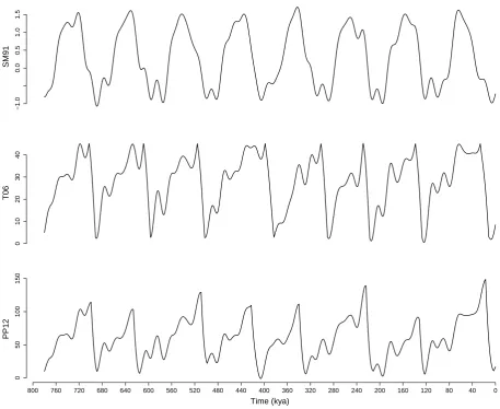
A comparison of the ice volume generated from the deterministic version of each model is shown in
Figure 2, using the parameters suggested in the original publications. Each model captures the broad
structure of the glacial-interglacial cycle. These plots are not precise reproductions of the figures in
the original publications, due to differences in the initial conditions and astronomical solutions. Note
that each model was tuned using a different dataset, and so, for example, SM91 has seven cycles in
780 kyr rather than eight.
Figure 2 about here.
2.4. Statistical observation model
The final modelling ingredient is a statistical model relating the state variables in the dynamical
τm is the estimated age andYm the measured proxy of the mth data point/slice. We use the model
Ym∼ N(D+HHH⊤XXXm, σ2y),
where we defineXXXm =XXX(τm). As with the choice of stochastic driver, we have assumed the simplest
observation model, and more complex observation models could be considered. Here, we use HHH = (C,0, . . . ,0)⊤, so that Y
m is a scaled and shifted version of the value X(1)(τm), the ice volume in
the underlying dynamical model. However, vector observations can be used at no additional cost or
complication to the methodology, allowing observations of other proxies if desired.
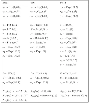
2.5. Prior distributions
A Bayesian approach requires specification of prior distributions for the parameters in each of the
models. Milankovitch theory suggests that a positive northern hemisphere insolation anomaly in
sum-mer increases ablation over the ice sheets, giving a negative contribution to the ice volume derivative
(Berger and Loutre, 2004). This requires thatγP andγE be positive, and so we use exponential prior
distributions on these parameters to allow the system to be weakly forced. Whether having more
insolation in spring at the expense of autumn should result in a positive or negative contribution
to ice accumulation is undetermined, and so we use a zero-mean Gaussian prior distribution for γC,
as this is symmetric about zero, which indicates Summer solstice insolation. Beyond these choices,
specifying prior distributions on physical grounds is difficult, as many of the model parameters do
not represent measurable quantities. In general we select moderately informative prior distributions
that discourage non-oscillating regimes, excessively small or large periods, and numerical instabilities.
The complete set of prior distributions for all three models is given in Table 1. Sensitivity to the
choice of prior distributions is investigated in Section 4.
Since we are performing model comparison, we have made the prior distributions as consistent
as possible across models. For instance, since we scale the output from each model, the observation
error variance, σ2y, is comparable, and so we use the same prior distribution for σy2 in each model. Care needs to be taken when selecting prior distributions for the astronomical forcing terms as each
model has a different scale for ice volume. From trial runs the range ofX(1) in PP12 is approximately 2.5 times that of T06, and 50 times that of SM91. Additionally, SM91 has a reference value for tof
10 kyr (as opposed to 1 kyr in T06 and PP12), suggesting a ratio of 1:2:5 for the astronomical forcing
parameters between SM91, T06, and PP12 respectively. This relationship is represented in the prior
distributions. Since this ratio is only approximate, we investigate sensitivity to this scaling rule in
Section 4.
3. Methodology
Our primary aim is model comparison, in particular to answer the question: given a collection
of competing models {Ml}Ll=1, which is best supported by the data? The Bayes factor (BF) for
comparing two models, M1 and M2 say, is the ratio of their evidences
B12= π(Y1:M | M1) π(Y1:M | M2) ,
where Y1:M = (Y1, . . . , YM) and where π(Y1:M | Ml) is the evidence for model Ml (Jeffreys, 1939;
Kass and Raftery, 1995). The Bayes factor summarises the strength of evidence in the data in support
of one model over another, and is the ratio of the posterior to the prior odds in favour of M1 over
M2. If the prior probabilities for each model are equal, then the Bayes factor is the ratio of the posterior model probabilities. There are many other approaches to model comparison, many of which
are based on measures of predictive accuracy such as cross-validation (see Vehtari and Ojanen (2012)
and Gelman et al. (2014)). Most of these approaches cannot be used in problems with complex data
dependencies, such as serial correlation. Ando and Tsay (2010) describe an approach that can be
used, but which requires calculation of the Hessian matrix of the log-likelihood. Additionally, many
of these methods require evaluation of quantities which may not be available for complex state space
models. For these reasons, and because our focus is on model comparison rather than on evaluating
predictive accuracy, we prefer to use Bayes factors to perform model comparison.
Secondary aims of our analysis include parameter estimation and filtering, which in this context
are often called calibration and climate reconstruction. Calibration is the process of finding the
posterior distribution of the model parametersπ(θθθl|Y1:M,Ml), whereθθθl is the parameter for model
Ml, and filtering is finding the distribution of the state variablesπ(XXX1:M |Y1:M, θθθl,Ml). These three
problems are of different levels of difficulty. Filtering is the most straightforward, but is not simple as
for non-linear or non-Gaussian models, direct calculation of the filtering distributions is not possible,
and so we must instead rely upon approximations. Calibration requires that we integrate out the
dependence on the state variablesXXX1:M,
π(θθθl|Y1:M,Ml) =
∫
π(θθθl, XXX1:M |Y1:M,Ml)dXXX1:M,
and hence, is considerably more difficult than filtering. Finally, model selection requires integrating
out the dependence onθθθl,
π(Y1:M | Ml) =
∫
π(θθθl| Ml)
∫
π(XXX1:M |θθθl,Ml)π(Y1:M |θθθl, XXX1:M,Ml)dXXX1:Mdθθθl,
and is thus even more difficult than calibration.
The development of Monte Carlo methodology for solving these three problems for state space
models reflects this hierarchy of difficulty. Particle filter methodology, first proposed in the 1990s
ofXXX1:M is not too large. Whereas the calibration problem has only begun to be satisfactorily answered
more recently, with the development of pseudo-marginal methods such as particle-MCMC (Andrieu
et al., 2010). Calculating the model evidence is, however, still very much an open problem.
Here, we demonstrate how the recently introduced SMC2 algorithm (Chopin et al., 2013) can be
used to estimate model evidences. The approach relies upon the following identities decomposing the
evidence:
π(Y1:M) =π(Y1) M
∏
m=2
π(Ym|Y1:m−1), (2)
and
π(Ym |Y1:m−1) = ∫
π(Ym |Y1:m−1, θθθ)π(θθθ|Y1:m−1)dθθθ, (3)
where we have dropped the dependence onMlfrom the notation. SMC2 can be used to sample from
π(θθθ | Y1:m−1), find unbiased estimates of π(Ym | Y1:m−1, θθθ), and, by plugging these estimates into
Equations (2) and (3), obtain an estimate of the model evidence, from which we can estimate the
Bayes factors.
3.1. Estimating Model Evidence Using SMC2
Sequential Monte Carlo algorithms (SMC) (Del Moral et al., 2006) are population-based sampling
methods that aim to sample from some target distribution,πM, by sampling from a series of
interme-diary distributions,{πm}Mm=1, that are chosen to gradually ‘close-in’ on the target distribution. SMC uses a weighted collection of particles to approximate each distribution, and sequentially updates the
weights and the particles in such a way that the normalising constant of each distribution can be
estimated. A common choice for the sequence of distributions is to add a single data point at a time,
so that the intermediary distributions areπ(θθθ|Y1:m) orπ(XXX1:m |Y1:m), for example.
One of the earliest SMC algorithms is the particle filter (PF) (Gordon et al., 1993), which
sam-ples from the sequence of filtering distributions πm(XXX1:m) = π(XXX1:m | Y1:m, θθθ), and is described in
Algorithm 1. The basic idea is that at initialisation, a sample ofNx particles are sampled from some
initial proposal density r1(XXX1 | Y1, θθθ), and given importance weight π(XXX1, Y1 |θθθ)⧸r1(XXX1 | Y1, θθθ). These particles are then repeatedly resampled using a multinomial scheme, propagated via some
ar-bitrary proposal distribution rm(XXXm |XXX1:m−1, Y1:m, θθθ), and reweighted accordingly, so that for each
successive iteration the particles are a weighted sample of the posteriorπ(XXX1:m |Y1:m, θθθ). Details of
the resampling and the proposal distributions, rm, are discussed in Section 3.2, and further details
can be found in Doucet and Johansen (2009).
An important aspect of the PF is that an unbiased estimate of the normalising constantπ(Y1:m |θθθ)
can be estimated from the unnormalised weights in each iteration of the algorithm, using
ˆ
π(Ym |Y1:m−1, θθθ) = 1 Nx
Nx
∑
k=1 ω(k)
m (XXX
Algorithm 1 Particle filter targeting π(XXX1:M |Y1:M, θθθ).
for k= 1, ..., NX do
SampleXXX(1k) ∼r1(XXX1 |Y1, θθθ). Set the importance weight
ω(1k)=
π(XXX(1k)|θθθ)π(Y1 |XXX(1k), θθθ )
r1 (
X
XX(1k) |Y1, θθθ
) .
end for
Normalise the weights. For k= 1, ..., NX
Ω(1k) = ω (k) 1 ∑NX
i=1ω (i) 1
.
for m= 2, ..., M do for k= 1, ..., NX do
Sample ancestor particle indexa(mk−)1 according to weights Ω(1:NX)
m−1 . SampleXXX(mk)∼rm
(
XXXm|XXX( a(mk)−1)
m−1 , Ym, θθθ
)
.
Extend particle trajectoryXXX(1:km) =
{ X XX(a
(k)
m−1)
1:m−1, XXX (k)
m
}
.
Set the importance weight
ω(mk)=
π (
XXX(mk)|XXX( a(mk−)1)
m−1 , θθθ )
π(Ym|XXX(mk), θθθ
)
rm
( X X
X(mk)|XXX( a(mk)−1)
m−1 , Ym, θθθ
) . (4)
end for
Normalise the weights. Fork= 1, ..., NX
Ω(k)
m =
ω(mk)
∑NX
i=1ω (i)
m
.
as an approximation to Equation (3), and then plugging these estimates into Equation (2) (Del Moral,
2004)
ˆ
π(Y1:M |θθθ) = ˆπ(Y1) M
∏
m=2 ˆ
π(Ym|Y1:m−1, θθθ). (5)
In Andrieu and Roberts (2009), it was shown that using these unbiased estimates of the likelihood
in other Monte Carlo algorithms can lead to valid Monte Carlo algorithms (termed pseudo-marginal
algorithms) for performing parameter estimation. For example, PMCMC (Andrieu et al., 2010) uses
the PF within an MCMC algorithm, and SMC2 (Chopin et al., 2013) uses a PF embedded within an
SMC algorithm, both with the aim of finding π(θθθ |Y1:M). We concentrate on the latter as it allows
for estimation of BFs.
The SMC2 algorithm (Chopin et al., 2013) embeds the particle filter within an SMC algorithm
targeting the sequence of posteriors
π0 =π(θθθ), πm=π(θθθ, XXX1:m|Y1:m),
form= 1, . . . , M. This is achieved by initially samplingNθ parameter particles,{θθθ(n)}Nn=1θ , from the
prior. To eachθθθ(n), we attach a PF of N
x particles, i.e., at iterationm the PF {XXX1:(k,nm),Ω(mk,n)}Nk=1x is
associated withθθθ(n), where Ω(k,n)
m are the normalised weights in Algorithm 1. From this PF we can
obtain an unbiased estimate of the marginal likelihoodπ(Y1:m |θθθ(n)) via Equation (5). To assimilate
the next observationYm+1, we first extend the PF for the state particles to{XXX(1:k,nm+1) ,Ω (k,n)
m+1}
Nx
k=1, and then estimate π(Y1:m+1 | θθθ(n)) and so on. Particle degeneracy occurs when the weighted particle approximation is dominated by just a few particles (i.e., a few have comparatively large weights), and
is monitored by calculating the effective sample size (ESS)
ESS =
(∑Nθ
i=1 (
Wm(i))2 )−1
,
where{Wm(i)
}Nθ
i=1are the normalised weights in populationm. When the ESS falls below some thresh-old (usually Nθ/2) the particles are resampled to discard low-weight particles. However, resampling
can lead to too few unique particles in the parameter space. Particle diversity is improved by
run-ning a PMCMC algorithm that leaves π(θθθ, XXX1:m |Y1:m) invariant, specifically the particle marginal
Metropolis-Hastings (PMMH) algorithm (Andrieu et al., 2010). The full details of the SMC2
algo-rithm are presented in Algoalgo-rithm 2, with theoretical justification in Chopin et al. (2013).
The model evidence π(Y1:M) can be decomposed according to Equation (2), and in each iteration
of the SMC2 algorithm, the term
ˆ
π(Ym|Ym−1) =
Nθ
∑
n=1
W(n)πˆ(Y
m|Y1:m−1, θθθ(n))
provides an estimate of π(Ym |Ym−1). An estimate of the model evidenceπ(Y1:M) is then obtained
Algorithm 2 SMC2 algorithm targeting π(θ, X1:M |Y1:M).
for n= 1, ..., Nθ do
Sampleθθθ(n) from the prior distribution,π(θθθ). Set the importance weight
W0(n)= 1 Nθ
.
end for
for m= 1, ..., M do if ESS< Nθ
2 then
for n= 1, ..., Nθ do
Sampleθθθ∗(n) andXXX∗(1:NX,n)
1:m−1 fromθθθ(1:N
θ)
andXXX(1:NX,1:Nθ)
1:m−1 , according to weightsW (1:Nθ)
m−1 . Sampleθθθ∗∗(n) andXXX∗∗(1:NX,n)
1:m−1 from a PMMH algorithm targetingπ(θθθ, XXX1:m−1|Y1:m−1) ini-tialised withθθθ∗(n) andXXX∗(1:NX,n)
1:m−1 .
end for
Setθθθ(1:Nθ)=θθθ∗∗(1:Nθ) andXXX(1:NX,1:Nθ)
1:m−1 =XXX
∗∗(1:NX,1:Nθ)
1:m−1 . Set the importance weights
Wm(n−)1= 1 Nθ
forn= 1, ..., nθ.
end if
for n= 1, ..., Nθ do
Sample XXX(1:NX,n)
1:m by performing iteration m of the particle filter, and record estimates of
ˆ
π(Ym|Y1:m−1, θθθ(n))and ˆπ(Y1:m |θθθ(n)
)
.
Set the importance weights
w(n)
m =W
(n)
m−1πˆ (
Ym|Y1:m−1, θθθ(n) )
.
end for
Evaluate
ˆ
π(Ym |Y1:m−1) =
Nθ
∑
i=1 w(mi)
Normalise the weights
Wm(n)= w (n)
m
∑Nθ
i=1w (i)
m
for n= 1, ..., Nθ.
3.2. Guided proposals
A further difficulty arises as the transition densities π(XXXm | XXXm−1, θθθ) are not available in closed form for the models of interest, suggesting that we need to choose the particle proposal distributions,
{rm}, so that the transition density cancels from the importance weights. This can be achieved by
settingrm =π(XXXm|XXXm−1, θθθ) in Equation (4), so that proposals are just simulations from the model. However, this choice will typically lead to particle degeneracy if too many of the proposals end up
being far from the observations, due to the light Gaussian tails in the observation model. Resampling
the state particles ensures that important particles are propagated forward, which can improve the
approximation in later iterations. Multinomial resampling is the most commonly used resampling
scheme, but alternatives such as stratified resampling give improvements in sample variance (Liu and
Chen, 1998; Douc et al., 2005).
For the SDE models considered here, resampling is not sufficient to overcome the degeneracy
problem. Our solution is to avoid using the model as the proposal distribution, and to instead build
novel Brownian bridge type proposals, based on the proposals developed in Golightly and Wilkinson
(2008), that guide the particles toward the next data point (thus decreasing degeneracy). The key
is to exploit the Euler-Maruyama approximation we use to simulate from the underlying SDE, in
order to condition the proposal distribution on the next observation, thus increasing the number of
proposals with large weights. Each of our models are SDEs of the form
dXXX(t) =µµµ(XXX(t), θθθ) dt+Σ
1 2
X(XXX(t), θθθ) dWWW (t).
The Euler-Maruyama approximation simulates from the SDE over time interval ∆t by partitioning the interval intoJ sub-intervals of lengthδt= ∆Jt, and using the discrete time equation
X X
X(t′+δt)=µµµ(XXX(t′), θθθ)δt+Σ
1 2
X
(
XXX(t′), θθθ)δt12ϵϵϵt,
whereϵϵϵt is a vector of independent standard Gaussian random variables. Simulating from the
dis-crete time equation between two observation times, τm and τm+1, introduces (J−1)×d latent variables, XXXm−1,1, ..., XXXm−1,J−1, where we let XXXm,j = XXX(τm+j·δt). We can extend the
parti-cle filter to also sample from these latent variables, by using a proposal distribution of the form
˜
rm+1(XXXm,1, ..., XXXm,J |Ym+1, XXXm, θθθ). The importance weight calculation in the particle filter is then
ω(mk+1) =
∏J
j=1π(XXXm,j |XXXm,j−1, θθθ)π(Ym+1 |XXXm+1, θθθ) ˜
rm(XXXm,1, ..., XXXm,J |Ym+1, θθθ)
,
where theπ(XXXm,j |XXXm,j−1, θθθ) are now assumed to be Gaussian densities.
We can guide the particles into regions of high likelihood by conditioning the value ofXXXm,j+1 on future observation, Ym+1. This can be done by approximating the distribution of Ym+1 conditional on XXXm,j using a single Euler-Maruyama step of size ∆ft = ∆t−jδt. To do this conditioning, note
that under an Euler-Maruyama step of interval size∆ft,
XXXm+1 |XXXm,j, θθθ∼ Nd
( X X
Xm,j+µµµm,j∆ft,Σm,j∆ft
where µµµm,j =µµµ(XXXm,j, θθθ) and Σm,j =ΣX(XXXm,j, θθθ). We can then see that the joint distribution of
XXXm,j+1 and Ym+1, givenXXXm,j, is
XXXm,j+1 Ym+1
|XXXm,j, θθθ∼ Nd+1
XXXm,j+µµµm,jδt H
HH(XXXm,j+µµµm,j∆ft
)
+D ,
Σm,jδt Σm,jHHH⊤δt H
H
HΣm,jδt HHHΣm,jHHH⊤∆ft+σ2y
.
Conditioning this distribution onYm+1 (Eaton, 1983), then suggests proposals of the form
X X
Xm,j+1|XXXm,j, Ym+1, θθθ∼ Nd(MMMm,j,SSSm,j),
where
M M
Mm,j =XXXm,j+µµµm,jδt+BBB⊤AAA−1
(
Ym+1−HHH (
XXXm,j+µµµm,j∆ft
)
−D),
and
SSSm,j =Σm,jδt−BBB⊤AAA−1BBB,
with
AAA=(HHHΣm,jHHH⊤∆ft+σy2
)
andBBB =HHHΣm,jδt.
In our experiments, we have found that using these guided proposals dramatically reduces particle
degeneracy. This improves the likelihood estimates, thus increasing the efficiency of the algorithm.
Consequently, smaller value of Nx (fewer state particles) can be used, and the PMMH rejuvenation
step has better mixing properties, allowing for shorter chains.
3.3. Further details
The tuning parameters are the number of particles,NθandNx, and the proposal distributions for the
PMMH rejuvenation steps. Typically,Nθ will be decided by the available computational resource. A
low value ofNxcan be used for early iterations, but must be increased when using longer time series of
data in later iterations. An insufficient number of state particles has a negative impact on the PMCMC
acceptance rate, leading to fewer acceptances. This will be reflected in a low particle diversity (the
number of unique particles), which needs to be monitored throughout. Automatic calibration ofNx
is discussed in Chopin et al. (2013), where it is suggested thatNxis doubled whenever the acceptance
rate of the PMCMC step becomes too small. We useNx =Nθ = 1000 throughout. The fact that we
have a collection of particles in each iteration allows automated calibration of the PMMH proposals.
For example, using the sample mean and variance to design a random-walk proposal, or using a
Gaussian independence sampler. We use independent Gaussian proposals using the sample mean
and covariance, with a chain length of 10 to maintain a high particle diversity. In the first iteration,
the proposal r1(XXX1 |Y1, θθθ) in the particle filter is taken to be the state prior distributions. In later iterations, for the continuous state variables we again use independent Gaussian proposals using
the sample mean and covariance, and for the discrete state variables we use independent Bernoulli
maximum (minimum) of 0.95 (0.05). Finally, we check if the algorithm has converged by ensuring
that the results are consistent between independent runs.
4. Results
4.1. Simulation study
In order to gain confidence in the ability of our SMC2algorithm for both model selection and
calibra-tion, we begin with a simulation study. We simulate a single random trajectory from a given model
and parameter setting and draw observations from the observation process. We then show that the
posterior distributions recover the true value of the parameters (Figure 3) and the true underlying
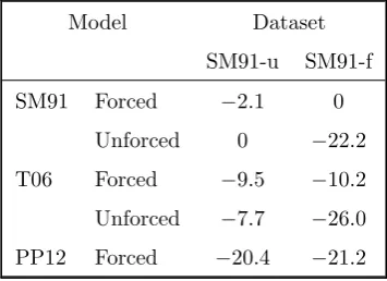
state (Figure 4), and that the Bayes factors correctly identify the true generative model (Table 2).
Further simulation studies and details are available in Carson (2015).
We present results from two datasets simulated from SM91: one in which data are from an
unforced version, denoted SM91-u, in which parameters γP = γC = γE = 0 so that F = 0, and a
forced version, SM91-f, for which these parameters and F are non-zero. The parameter values used were: p = 0.8, q = 1.6, r = 0.6, s= 1.4, v = 0.3, σ1 = 0.2, σ2 = 0.3, σ3 = 0.3, D = 3.8, S = 0.8, σy = 0.1, and additionally for SM91-fγP = 0.3,γC = 0.1,γE = 0.4, which are comparable with those
estimated from real data. We simulate observations every 3 kyr over the past 780 kyr to give 261
observations in each dataset, comparable to a low resolution sediment core. From these datasets we
calculated the model evidence and posteriors for each of five models: the forced and unforced versions
of SM91 and T06, and the forced model PP12. We do not consider an unforced PP12 model because
the deglaciation-glaciation transition depends only on the astronomical forcing (whereas SM91 and
T06 both oscillate in the absence of any external forcing). The models contain between 10 and 16
parameters. The priors used for each model are given in Table 1.
The estimated log10 Bayes factors (log10BF) are given in Table 2. A common interpretation
sug-gests that log10B12>0.5 is substantial evidence in favour of modelM1over modelM2, log10B12>1 is strong evidence thatM1 is superior, and log10B12>2 is very strong evidence (Kass and Raftery, 1995). Conversely, a negative score indicates the same strength of evidence but in the other direction
(for M2 over M1). In each column, the log10 BF is with respect to the true generative model, so
that positive values indicate support for that model over the true model, and negative values indicate
support for the true model. Because the log10 BF is just the difference between the log evidences,
we can reconstruct the evidences by noting that the log10 evidence (log10π(y1:M|M)) is 29.8 for the
unforced version of SM91 on the SM91-u dataset, and 40.7 for the forced SM91 model on the SM91-f
dataset.
Table 2 about here.
SM91-f, the correct model (the forced SM91 model) is overwhelmingly favoured. The log10 BF to
the next most supported model (the forced T06 model) is estimated to be 10.2, indicating decisive
evidence in favour of the true model. It is interesting to note that if we remove the forced SM91 model
from the analysis, we find decisive evidence in favour of the forced T06 model over any of the other
unforced models (a log10 BF of at least 11), showing that the astronomical forcing has explanatory
power even in the wrong model (to find other BFs, note that logBij = logBi0−logBj0). This is not particularly surprising, because in both models the astronomical forcing acts as a synchronisation
agent, controlling the timing of terminations, and has a strong effect on the likelihood. This is a
reassuring finding: it suggests that paleoclimate scientists can implicitly rely upon this effect when
arguing for the importance of the astronomical forcing, as it allows us to infer its importance even
when using an incorrect model (for we surely are).
When applied to SM91-u the log BF again correctly identifies the correct generative model,
al-though the support for the unforced and forced SM91 models is now much closer (with a log10 BF of
2.1 in favour of the unforced model). In cases where the forcing does not add any explanatory power
this is an expected result, as the unforced version of SM91 is nested within the forced version, and
can be recovered by setting γP = γC = γE = 0. This effect is also noticeable when comparing the
forced and unforced T06 models, with the unforced version being preferred with a log10 BF of 1.8.
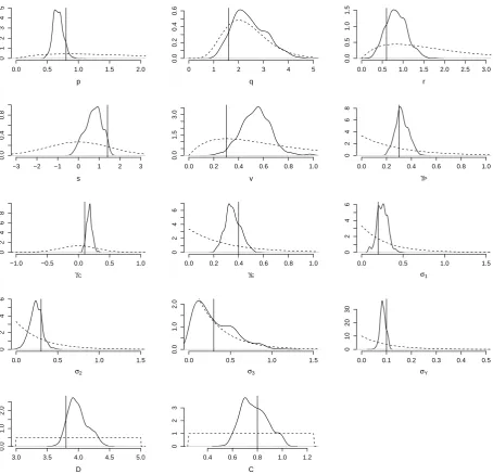
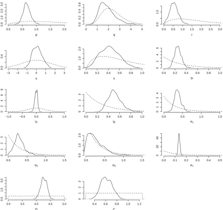
The marginal posterior distributions for the parameters for the forced SM91 model applied to the
SM91-f dataset are shown in Figure 3. We are able to recover the parameters used to generate the
data, with the true values lying in regions of high posterior probability. The posteriors forq and σ3
do not deviate much from the prior, suggesting that a wide range of values explain the data equally
well.
Figure 3 about here.
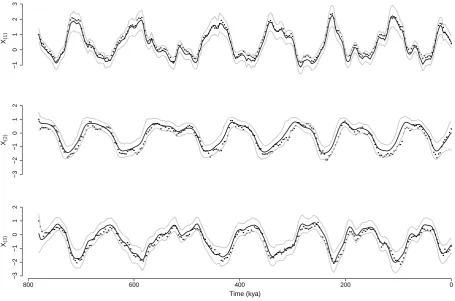
Finally, the sequence of 95% highest density regions (HDRs) for the state estimates for the forced
SM91 model applied to the SM91-f dataset are shown in Figure 4. For each of the three states, most
of the true values lie within the HDRs, demonstrating that we are able to recover the state of the
system, despite only having noisy observations of a single state.
Figure 4 about here.
4.2. ODP677
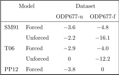
We now analyse dataset ODP677 from the ocean drilling programme (ODP). The estimated log10
BFs for each model are given in Table 3. We use ODP677-u to refer to age model estimates derived
by Huybers (2007) using a depth derived model, and ODP677-f to the astronomically tuned age
model estimates described in Lisiecki and Raymo (2005). The BFs are given in comparison to the
evidence of 28.2. The results suggest strong evidence in favour of the unforced models over the forced
models, which are penalised for containing extra parameters with little explanatory power. That the
unforced model is preferred may be surprising compared to earlier works based on similar records
(Raymo, 1997; Huybers, 2011); this is discussed further in the conclusions.
Table 3 about here.
When we analyse ODP677-f, the astronomically tuned data, the results are reversed. We now find
strong evidence in favour of the PP12 model (with a log10evidence of 33.7), and that the three forced
models are all decisively preferred to the two unforced models, i.e., we find overwhelming evidence
using these data that astronomical forcing is necessary to explain the data. The orbital tuning of
ODP677-f is the most likely explanation for this. There is some evidence that T06 is more strongly
supported than SM91 with a log10BF of 0.8.
This result is our second key finding. Namely, that inference about the best model is affected by the
age model used to date the data. It is vital that modelling assumptions in the dating methods should
be understood when performing inference on paleoclimate data. Given that the two chronologies,
ODP677-f and ODP677-u, are considered consistent once we account for dating uncertainties, we
suggest that this formally demonstrates that the approach of first dating the data, and then carrying
out down-stream analyses given this dating (ignoring the uncertainty) may undermine any subsequent
inference about the dynamic mechanisms at play.
Whilst these results demonstrate that the age model strongly influences the conclusions in model
comparison experiments, care must be taken to not over-interpret the results. Bayes factors are
sensitive to changes in the prior distributions, and in this case, are subject to Monte Carlo error. It
is possible that selecting new prior distributions consistent with our approach in Section 2.5, or even
keeping the same prior distributions and reinitialising the algorithm with a different seed could result
in different conclusions. This is investigated in the next section.
The marginal posterior distributions of the parameters in the SM91 model when fit to the
ODP677-f data are shown in Figure 5. The astronomical ODP677-forcing scaling parametersγP andγE have very small
posterior support at 0, suggesting that both precession and obliquity are important.
Figure 5 about here.
Figure 6 provides the density of the ratios
√
γ2 P+γ
2 C
γE , and the argument of the complex number
γP +iγC for SM91 and T06. PP12 is omitted as the truncation of the forcing makes the parameters
incomparable. The rationale for using arg(γP +iγC) can be made clear by noting that the forcing
(Equation 1) can be reformulated as
F(t;γγγ) = Γ sin(ϖ(t) +ϕ) +γEE(t),
where Γ ∝ |γP +iγC| and ϕ = arg(γP +iγC) (the proportionality is straightforwardly set by the
process of precession of equinoxes, whileϕcontrols the phase. It follows that the ratio γΓE =
√
γ2 P+γC2
γE
measures the relative weight in the forcing of two different physical effects: the precession of equinoxes,
and the changes in the tilt of the Earth’s equator (obliquity). The results in the left plot of Figure 6
are consistent across models, with a ratio lower than one, suggesting that the control of obliquity
dominates. Translated in terms of paleoclimate dynamics, this means that ice age dynamics are
controlled by insolation integrated over a season length, rather that just the maximum insolation over
the year. The right plot in Figure 6 shows the argument of the complex numberγP+iγC. Here, zero
means that phase of the precession forcing matches that of the June solstice insolation. A phase ofπ/2 would mean that the system is controlled by March insolation, while−π/2 would point to September insolation. All densities are broadly centred on zero, suggesting a summer insolation control in
the Northern Hemisphere (this is also consistent with a winter control in the Southern Hemisphere,
but this is less plausible). The nominal uncertainty of approximately 0.8 radians translates into an
uncertainty of about 2 months in calendar time. Physically, it is reasonable to assume that the
driving effect changes as ice sheets grow and melt, and that these changes contribute to the variance
of the density curves. We acknowledge that dating assumptions will also presumably be crucial in
determining this quantity.
Figure 6 about here.
4.3. Robustness
The simulation studies show that there is sufficient information in the observations to easily detect
the correct parametric form of the model in each case. However, the Bayes factors are sensitive to
both Monte Carlo error in the evidence estimates, the choice of prior distributions, and model
mis-specification, and so care needs to be taken when using real data in order to avoid over-interpretation.
To investigate the Monte Carlo error in the Bayes factor estimates, we calculate the model
ev-idences for the forced models on ODP677-f using ten randomly generated seeds for each model.
The log10 evidences were in the range [28.4,29.0] for SM91, [29.4,31.5] for T06, and [33.3,34.2] for PP12. Over all repeats PP12 is still strongly favoured, but not necessarily decisively favoured (as the
log10BF is as small as 1.8). Likewise, T06 is favoured over SM91, but not necessarily substantially
favoured (as the log10BF is as small as 0.4). Forced models are still decisively favoured over unforced
models. The implications for the experiment on ODP677-u are that each of the forced models are
plausibly equally well supported by the data, and further confirming that the difference between the
forced and unforced version of the same parametric model is small. The magnitude of the estimation
error can be decreased by using more particles in the SMC2 algorithm, but this will require very long
computational runs. UsingNx=Nθ= 1000 takes 3-4 days on a standard desktop depending on the
model. However, SMC algorithms are well suited to run in parallel, and we were able to obtain a
To test the robustness of our conclusions to changes in the prior distributions, we performed a
sensitivity analysis using the two ODP-677 datasets. Kass and Raftery (1995) advocate recomputing
the Bayes factors with perturbed hyperparameters, for example by halving/doubling scale and
vari-ance parameters. Given the computational expense of our experiments, it is not feasible to do this
one parameter at a time. Instead we conducted the following two experiments for the forced models.
In the first we maintained the 1:2:5 cross-model rules for the forcing prior construction (as discussed
in Section 2.5), but each of the other hyperparameters we halve or double with equal probability. For
the gamma distributions we maintain the prior means by doubling or halving the shape parameter
(exponential distributions are treated as gamma distributions with a shape parameter of 1 for this
purpose). In the second experiment we halve the hyperparameters for the astronomical forcing
pa-rameters only, and compare the results to those obtained in the initial experiment in order to violate
the 1:2:5 ratio. The aim of the first experiment is to investigate the sensitivity of our conclusions to
changes in the prior distributions for the model parameters, whereas the aim of the second is to test
the sensitivity to the cross-model assumptions made in Section 2.5.
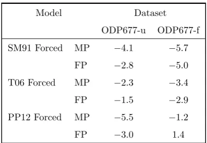
Table 4 about here.
The estimated log10 BFs of the new experiments are shown in Table 4, given with respect to
the best model from the first analysis for each dataset. We have denoted results from the first
sensitivity analysis as MP, to indicate that our focus is on the model parameters, and results from
the second sensitivity analysis as FP, as our focus is on the forcing parameters. It is difficult to
decouple the effect of changing the prior distributions from the Monte Carlo error, but the combined
change is within ±2 in each case. Taken together with the suggested interpretation of BFs in Kass
and Raftery (1995), this suggests the conservative rule-of-thumb that the log10 BF should be at least
5 to constitute strong evidence for one model over another if we are not confident about our choice of
prior distributions. If we revisit the results from the first analysis with this in mind, we find broadly
the same model comparison conclusions, i.e., unforced T06 is favoured in ODP677-u, and PP12 is
favoured in ODP677-f, even when the prior scaling rules designed in Section 2.5 are violated, but we
can no longer be confident that these results constitute strong evidence in favour of these models.
We still have strong evidence against unforced models for ODP677-f.
As our primary focus is on selecting between phenomenological models, we also need to consider
the impact of the modelling assumptions used for the stochastic driver and observation errors. In
particular, if these components are mis-specified, what will the effect be on the Bayes factors? To
test the robustness of the Bayes factors we revisit the simulation study datasets from Section 4.1 and
simulate additional sets of observations as follows. Firstly, we simply redraw observations (Y1:T) from
the trajectory generated for SM91-f (XXX1:T) in order to give a baseline for the Bayes factor variability
again from the same trajectory, using the AR1 process
ϵt+1=ρϵt+N (0, σ2),
withσ = 0.1, andρ= 0.6 (termed SS-AR06) and ρ= 0.9 (termed SS-AR09). The purpose of this is to test the robustness of the Bayes factors under a mis-specification of the observation error model.
We also generate two new trajectories from SM91-f, SS-JD78 and SS-JD780, using a jump-diffusion
instead of a Brownian motion as the stochastic driver of the SDE. The jump times are drawn from a
Poisson process with intensity 0.1 kyr−1 in SS-JD78, and 1 kyr−1 in SS-JD780, giving the expected
number of jumps as 78 and 780 respectively. The jump intensity is multivariate Gaussian with mean 0
and covariance matrix diag(0.22,0.32,0.32). This is 100 times the variance of a single Euler-Maruyama integration step of the Brownian motion, and equivalent to about 7-10% of the range of each state
variable. This allows us to test the robustness of the Bayes factors under a mis-specification of the
stochastic driver. Finally, we generate two datasets where we expect the Bayes factors to be weak,
in order to ensure that the results are not overconfident. In the first, termed SS-LE, we generate
observations using the same trajectory as SM91-f, but with large observation errors (increasing the
variance of the error 100-fold). In the second, termed SS-OU, we generate a trajectory using an
Ornstein-Uhlenbeck process (i.e., not using any of the phenomenological models). The datasets are
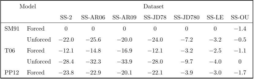
shown in Figure 7.
Figure 7 about here.
The estimated log10 Bayes factors (with respect to the best model) for our five models in each
of the seven new datasets are given in Table 5. We emphasise that care needs to be taken when
interpreting Bayes factors between different datasets: Bayes factors only indicate relative model
performance, and so we may obtain larger Bayes factors in instances where the correct model is not
in our library. This should not be interpreted as the preferred model being good in an absolute sense.
For SS-2, the model evidences change by a factor of 106 (cf. Table 2) and the Bayes factors change
by up to 2.6 on the log10 scale (some of this variability will be due to the Monte Carlo error), but
our conclusions are fundamentally unchanged. The exception is that the unforced SM91 model is
now preferred over PP12, but the Bayes factor between the two models is relatively small in both
simulation studies. In the AR1 datasets, T06 seems to perform poorly (the Bayes Factor between
SM91 and PP12 seems to be consistent with the original simulation study). A potential reason for this
is that the interglacial-glacial switches in T06 occur at some constant threshold for the state-variable,
whereas in the data there is greater variation in the local minima (particularly in SS-AR09). SM91
and PP12 seem to be more robust to this behaviour. For SS-JD78, the Bayes factors seem consistent
with the initial simulation study. This can partially be explained by the nature of oscillators such as
SM91, where trajectories following perturbations converge rapidly to a limit cycle, and so the overall
less predictable, indicating that the jumps have had some effect. For SS-JD780 the Bayes factors are
much weaker, and we can see in Figure 7 that the cycles are far less regular than the SM91 model
forced by Brownian motion. However, we still favour the forced SM91 model, suggesting that enough
information is preserved to allow us to pick out the correct model. For SS-LE (large observation error)
the order of the models is consistent with the previous simulation studies, but the Bayes factors are
much weaker, as expected. For SS-OU (data generated from an Ornstein-Uhlenbeck process), none
of our five candidate models are close to being useful, and consequently we find relatively small BFs
compared to previous simulation studies, but with the models ordered by their complexity (in terms
of the number of parameters), demonstrating Occam’s razor type behaviour of the Bayes factor.
Table 5 about here.
These are reassuring findings, in that the order of the models seem to be robust to moderate
mis-specifications of the stochastic driver and observation error model. In the limit where no model has
explanatory power, the Bayes factors favour the less complex models. It is plausible that significant
model mis-specification could bias the model selection to a significant extent, e.g., by favouring more
complex models to account for the mis-specification. Ideally alternative drivers and observation error
models would be considered, with Bayes factors used to select between candidates. However, each
would require the design of new proposal mechanisms in the particle filter, which is a non-trivial task.
5. Conclusions
We have two key conclusions. The first is that Monte Carlo methodology and computer power are
now sufficiently advanced that with work, it is possible to fully solve the Bayesian model selection
problem for a wide class of phenomenological models of the glacial-interglacial cycle. Using only 261
observations, we are able to learn up to 16 parameters, state trajectories containing 261×3 values,
and calculate the model evidence. Moreover, these evidences are sufficiently different (and able to
be estimated with sufficient accuracy) that we can discriminate between the ability of the models to
explain the data. However, care needs to be taken so as to not over-interpret the results from these
experiments. Firstly, Bayes factors are known to be sensitive to the prior distributions, and so the
conclusions might not be robust to changes in the priors. Fortunately, our analysis indicates that
useful results can still be obtained when the prior distributions are carefully elicited. Secondly, that
one dynamical system is more supported by the data than another does not necessarily imply that the
physical interpretation of that model is valid. At this level of conceptual modelling, different physical
interpretations may produce similar equations. This point has been made before (Tziperman et al.,
2006) and we add here that the stochastic differential equations emerge as a combination of judgements
on physical processesand model discrepancy, embedded in the stochastic parameterisations. On the