Exploring uncertainties in the relationship between temperature, ice volume, and sea level over the past 50 million years

BETWEEN TEMPERATURE, ICE VOLUME, AND SEA

LEVEL OVER THE PAST 50 MILLION YEARS

Edward Gasson,1,2Mark Siddall,1Daniel J. Lunt,3,4Owen J. L. Rackham,5Caroline H. Lear,6 and David Pollard7

Received 24 February 2011; revised 27 October 2011; accepted 30 October 2011; published 19 January 2012.

[1] Over the past decade, efforts to estimate temperature and sea level for the past 50 Ma have increased. In parallel, efforts to model ice sheet changes during this period have been ongoing. We review published paleodata and modeling work to provide insights into how sea level responds to changing temperature through changes in ice volume and thermal expansion. To date, the temperature to sea level rela-tionship has been explored for the transition from glacial to interglacial states. Attempts to synthesize the temperature to sea level relationship in deeper time, when temperatures were significantly warmer than present, have been tentative. We first review the existing temperature and sea level data and model simulations, with a discussion of uncertainty in each of these approaches. We then synthesize the sea level and temperature data and modeling results we have reviewed to test plausible forms for the sea level versus tempera-ture relationship. On this very long timescale there are no

globally representative temperature proxies, and so we inves-tigate this relationship using deep-sea temperature records and surface temperature records from high and low latitudes. It is difficult to distinguish between the different plausible forms of the temperature to sea level relationship given the wide errors associated with the proxy estimates. We argue that for surface high-latitude Southern Hemisphere tempera-ture and deep-sea temperatempera-ture, the rate of change of sea level to temperature has not remained constant, i.e., linear, over the past 50 Ma, although the relationship remains ambiguous for the available low-latitude surface temperature data. A non-linear form between temperature and sea level is consistent with ice sheet modeling studies. This relationship can be attributed to (1) the different glacial thresholds for Southern Hemisphere glaciation compared to Northern Hemisphere glaciation and (2) the ice sheet carrying capacity of the Ant-arctic continent.

Citation: Gasson, E., M. Siddall, D. J. Lunt, O. J. L. Rackham, C. H. Lear, and D. Pollard (2012), Exploring uncertainties in the relationship between temperature, ice volume, and sea level over the past 50 million years,Rev. Geophys.,50, RG1005, doi:10.1029/2011RG000358.

1. INTRODUCTION

[2] Understanding and predicting glacier and ice sheet dynamics is notoriously difficult [Alley et al., 2005;Allison et al., 2009], and as a result, in their fourth assessment report the Intergovernmental Panel on Climate Change did not provide sea level projections that accounted for rapid dynamical changes in ice flow [Solomon et al., 2007]. The observational record contains worrying examples of

nonlinear threshold type responses, such as the collapse of the Larsen B ice shelf and subsequent surging of glaciers [De Angelis and Skvarca, 2003;Rignot et al., 2004]. How-ever, the observational record does not help us constrain large changes to the ice sheets. Although there is no known analog to projected future warming in the paleoclimate record [Crowley, 1990;Haywood et al., 2011], it does con-tain examples of large-scale changes to the ice sheets [DeConto and Pollard, 2003a; Miller et al., 2005a]. The paleoclimate record can therefore aid understanding of ice sheet behavior and provide insight into the plausibility of large ice sheet changes in a warming world [Scherer et al., 1998; Pollard and DeConto, 2009]. By looking to the paleoclimate record we can also attempt to better understand the relationship between different climate parameters, such as temperature, atmospheric CO2, ice volume, and sea level

[Rohling et al., 2009]. 1

Department of Earth Sciences, University of Bristol, Bristol, UK. 2_{British Antarctic Survey, Cambridge, UK.}

3

BRIDGE, School of Geographical Sciences, University of Bristol, Bristol, UK.

4

Also at British Antarctic Survey, Cambridge, UK. 5

Bristol Centre for Complexity Sciences, University of Bristol, Bristol, UK. 6

School of Earth and Ocean Sciences, Cardiff University, Cardiff, UK. 7

Earth and Environmental Systems Institute, College of Earth and Mineral Sciences, Pennsylvania State University, University Park, Pennsylvania, USA.

Copyright 2012 by the American Geophysical Union. Reviews of Geophysics, 50, RG1005 / 2012 1 of 35 8755-1209/12/2011RG000358 Paper number 2011RG000358

[3] Over the past 50 million years,eustatic sea levelhas varied between 100 m above present in the early Eocene (56–49 Ma), when there was little or no land ice on Earth and the ocean basin volume was less than present [Miller et al., 2005a; Kominz et al., 2008; Miller et al., 2009a], and 120–140 m below present [Fairbanks, 1989;Yokoyama et al., 2000] during theLast Glacial Maximum(LGM; 19– 23 ka), when there were large ice sheets in Antarctica, North America, Asia, and Europe [Clark et al., 2009]. (Italicized terms are defined in the glossary, after the main text.) On this timescale, large (greater than 10 m) eustatic sea level varia-tions have been caused predominately by changes in the volume of land ice [Miller et al., 2005a]. Broadly, there have been four ice sheet states, these being (1) largely unglaciated conditions, (2) a glaciated East Antarctic, (3) interglacial conditions with additional ice sheets in the West Antarctic and Greenland (i.e., present-day conditions), and (4) glacial conditions with the additional growth of large ice sheets in the Northern Hemisphere [de Boer et al., 2012]. The gla-ciation of the East Antarctic can also be further broken down into an intermediate state with ephemeral mountain ice caps and a fully glaciated state [DeConto and Pollard, 2003a; Langebroek et al., 2009].

[4] The temperature range on this timescale is perhaps less well understood. Deep-sea paleoclimate proxies are com-monly used to interpret past climate changes as much of the regional and seasonal changes present in surface ocean and terrestrial records are reduced by the large volume and slow recycling of the deep ocean [Lear et al., 2000; Lear, 2007; Sosdian and Rosenthal, 2009]. Deep-sea temperatures (DSTs) in the early Eocene (50 Ma) may have been 7°C–15°C warmer than present, with a best estimate of 12°C [Lear et al., 2000; Zachos et al., 2001;Billups and Schrag, 2003; Lear, 2007]. The deep sea was1.5°C–2°C cooler than pres-ent during the LGM, with further cooling limited as tempera-tures approached the freezing point for seawater [Waelbroeck et al., 2002;Elderfield et al., 2010;Siddall et al., 2010a].

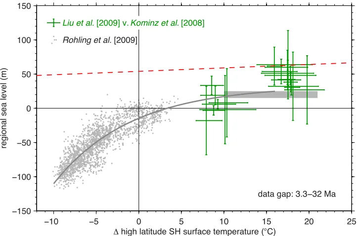
[5] Sea surface temperature (SST) proxies suggest that during the Eocene, the high latitudes were significantly warmer than present, approaching or even exceeding tem-peratures seen in the modern tropics [Bijl et al., 2009;Hollis et al., 2009; Liu et al., 2009;Bijl et al., 2010]. However, the lower latitudes were only a few degrees warmer than present in the Eocene [Sexton et al., 2006;Lear et al., 2008; Keating-Bitonti et al., 2011], suggesting that there was a much reduced latitudinal temperature gradient [Huber, 2008; Bijl et al., 2009]. During glacial conditions, the surface high latitudes show cooling [Jouzel et al., 2007], with this cooling also extending to low latitudes, suggesting that there were additional feedbacks on the climate system, such as CO2

feedbacks, in addition to orbital driven forcing [Herbert et al., 2010;Rohling et al., 2012].

[6] Over the past 50 Ma there have also been major tec-tonic changes, such as the uplift of the Himalayas following the collision of India with Asia, the opening of the Drake and Tasman passages, and the closing of the Panama sea-way, which have all had an influence on the climate system [Zachos et al., 2001].

1.1. Temperature to Sea Level Relationship

[7] Surface temperature is related to sea level through its control on the amount of ice stored on land and through thermal expansion. Sea level response to temperature forcing over the past 0.5 Ma has been studied using proxy data from ice cores, ocean sediments, and fossil corals [Rohling et al., 2009; Siddall et al., 2010a, 2010b]. However, for longer periods (106–107years), only modeled estimates have been published, albeit constrained by data [de Boer et al., 2010]. Here we use existing proxy records from the past 50 Ma to investigate the relationship and uncertainties between tem-perature and sea level during the transition to an“ice house” world. There are no globally representative temperature proxies on this timescale; instead, we investigate the rela-tionship using DST and surface temperatures from high and low latitudes.

[8] When looking at this long time period, the proxy record of surface temperature is limited in both duration and spatial coverage, although records are improving with the continued development of new and existing proxies [Lear et al., 2008; Liu et al., 2009]. A limitation of using iso-lated surface temperature proxies is that there are inherent uncertainties as to whether regional and/or seasonal tem-perature fluctuations are being recorded [Lear et al., 2000]. These potential biases are reduced in the DST record, although the DST record has other significant limitations [Lear et al., 2000; Billups and Schrag, 2003]. DST is coupled to SST at regions of deep-water formation, which for the present day are predominantly, although not exclu-sively [Gebbie and Huybers, 2011], the high latitudes [Zachos et al., 2001]. Therefore, DST proxies should not be seen as a record of past global temperature but should instead be viewed as analogous to past high-latitude surface temperature [Zachos et al., 2001]. The DST record is useful when investigating the sea level to temperature relationship, as it is best coupled to the surface at regions of ice formation.

1.2. Review Outline

[9] The majority of this review is focused on the DST to sea level relationship for the past 50 Ma, as the DST record is more complete than the surface temperature record. Additionally, we investigate the surface temperature to sea level relationship over a key interval for sea level change, theEocene-Oligocene transition (EOT). The direct transla-tion between the DST to sea level relatransla-tionship to the surface temperature to sea level relationship is dependent on the existence of a constant deep-sea to surface temperature gradient through time. We include a discussion of how the deep-sea to surface temperature gradient may have changed over the multimillion year timescale of this study because of changes in ocean circulation and changing sources of deep-water formation [Cramer et al., 2009;Katz et al., 2011].

1977;Exon et al., 2001] or global cooling through declining atmospheric CO2 [DeConto and Pollard, 2003a, 2003b;

Pagani et al., 2005]. However, a full discussion is beyond the scope of this review. Arguably, the more established hypothesis at present is that glacial inception on Antarctica resulted from global cooling, which was likely due to declining atmospheric CO2[DeConto and Pollard, 2003a,

2003b; Huber et al., 2004; Stickley et al., 2004; Pagani et al., 2005; Liu et al., 2009; Pearson et al., 2009]. First we review the available sea level, temperature, and model data, then we give a synthesis of the sea level relationship with DST and the sea level relationship with SST from high and low latitudes, and finally, we explore how this has affected understanding of the evolution of ice sheets over the past 50 Ma.

2. PROXY RECORDS

[11] Long-duration (107 years) records of sea level, ice volume, and temperature over the past 50 Ma are limited to ocean sediment deposits. Although other proxy records exist (e.g., from isotope analysis of fossil tooth enamel [Zanazzi et al., 2007] or sediment records from an incised river valley [Peters et al., 2010]), these are of a too short duration to be included in this review. Long-term (107years) records are presently limited tosequence stratigraphyrecords of sea level [Miller et al., 2005a],Mg/Ca proxy records of DST [Lear et al., 2000;Billups and Schrag, 2003], and records of oxygen isotopes (d18O), which are a mixed climate signal [Zachos et al., 2001]. Other proxies, such as the tetraether index (TEX86) and thealkenone unsaturation index(Uk′37), have been used to create intermediate-duration (106years) SST records.

2.1. Sequence Stratigraphy: A Sea Level Proxy

[12] Sequence stratigraphy ofpassive continental margins can provide a record of regional sea level over the past 50 Ma and even longer timescales [Vail et al., 1977; Haq et al., 1987; Miller et al., 2005a; Kominz et al., 2008]. Depositional sequences bounded by unconformities (periods of nondeposition and/or surfaces of erosion) show changes in regional sea level. By accurately dating sequences and inferring the past water depth during depositional phases from lithofacies and biofacies models, a quantitative esti-mate of sea level through time can be created (for a full discussion see Miller et al. [1998, 2005a], Kominz et al. [2008], andBrowning et al.[2008]).

[13] Vail et al. [1977] developed a method for inferring global sea level by correlating sequences from multiple depositional basins. This work led to the production of the

“Haq curve,”which was claimed at the time to be a global eustatic record of sea level [Haq et al., 1987].Miall[1992] was critical of the approach used byHaq et al.[1987] as it assumes that the dating of sequences is accurate enough to allow for correlation across multiple depositional basins. However, the duration of some of the sequences is often less than the age error estimate. Miall[1992] demonstrated that sequences created using a random number generator with the same age errors could generate a good correlation with the

Haq curve. It is unclear whether the sequences are the result of a global sea level signal or generated by regional pro-cesses, making correlation across multiple basins question-able [Christie-Blick et al., 1988]. Other criticism has focused on the lack of availability of data that made up the Haq curve, meaning that independent verification of the record is not possible [Miall, 1992]. Given these fundamental weak-nesses, Miall [1992] suggested that the Haq curve in par-ticular should be abandoned and efforts should be focused on independent well-dated records, such as those discussed in the following.

[14] Within the last 15 years, multiple well-dated sediment cores from one region, the New Jersey (NJ) margin in the northeastern United States, have been used to create a sequence stratigraphy record of sea level over the past 10– 100 Ma (sea level for 0–9 Ma in the study byMiller et al. [2005a] is estimated from a calibration of thed18O record as the NJ sequence stratigraphy record is incomplete from 0 to 7 Ma) [Miller et al., 2005a;Kominz et al., 2008] (see Figure 1). By taking into account compaction, loading, and subsidence of the sediment core (thebackstrippingmethod), a regional sea level record was created [Browning et al., 2008]. The sequences are dated using a combination of biostratigraphy,magnetostratigraphy, and strontium isotope stratigraphy, providing age control better than 0.5 Ma [Kominz et al., 2008], which is a significant improvement on the3 Ma age errors of the Haq curve [Miall, 1992].

[15] When regional sea level drops below the level of the core hole site, there is a hiatus in the record, identified as an unconformity. This is a potential limitation of sequence stratigraphy because it means water depth information is restricted during lowstands. This is overcome in part by having multiple core hole locations from both onshore and offshore sites; however, there are still significant hiatuses in the composite record during lowstands. Although a quantitative record of water depth is limited during low-stands, it is likely that sea level was lower than surrounding highstands given the lack of sediment deposition. As shown in Figure 1, Kominz et al. [2008] provide “conceptual” lowstands, which highlight that sea level is lower during periods when there are no deposits; errors during these per-iods are significantly higher than during highstands. Here we assume generous errors of50 m during lowstands, based on the highest error estimate of Miller et al. [2005a]. The highstand sea level estimate has an associated water depth error. The errors generally increase with increasing water depth; highstand errors for the NJ sea level record are typi-cally10–20 m [Miller et al., 2005a].

2007]. However, this is not directly relatable to the NJ sea level record. If this additional mass of water was added to the oceans, it would have anisostaticeffect (hydroisostasy), meaning that the sea level rise visible from NJ may be 33% less [Pekar et al., 2002; Miller et al., 2009a]. Therefore, assuming full isostatic adjustment (it should be noted that this hydroisostatic correction is not universally accepted [e.g.,Cramer et al., 2011]), only43–54 m of the long-term fall in the NJ record can be explained by the for-mation of the modern ice sheets [Pekar et al., 2002;Miller et al., 2005a]. Assuming that DSTs have cooled by12°C over the past 50 Ma (see below [Lear et al., 2000;Zachos et al., 2001]),12 m can be explained bythermostericsea level fall [Miller et al., 2009a]. This leaves an additional sea level fall, which by inference could be explained by an increase in ocean basin volume [Miller et al., 2009a].

[17] Ocean crust production rates may have decreased since the early Cenozoic [Xu et al., 2006]. Because seafloor becomes deeper as it ages, slower ocean crust production rate effectively increases ocean basin volume [Xu et al., 2006]. This is not consistent with the results of Rowley [2002], which suggested ocean crust production rates, and therefore ocean basin volume, have not varied significantly over the past 180 Ma. Müller et al. [2008] reconstructed ocean basin volume using marine geophysical data. Their data did suggest a decrease in sea level caused by an increase in ocean basin volume since 50 Ma of20 m. It should be noted that their reconstruction significantly differs from the NJ record on longer timescales [Müller et al., 2008], as discussed below. This combined total of 75–86 m does

not close the long-term NJ sea level budget and may suggest that the record contains other components.

[18] For multiple reasons, a sea level record from any single coastal area should be viewed as a record of regional sea level rather than a record of global eustatic sea level [Kominz et al., 2008]. This is because in addition to sea level changes resulting from the movement of water to and from storage as ice on land, the variation in the ocean basin vol-ume, and the thermal expansion of water, there are regional effects that may be recorded [Pekar et al., 2002]. If a con-tinental plate moves vertically, e.g., as a result of ice loading, this will be seen as a sea level change in the record [Peltier, 1974]. Isostasy due to ice loading will not have affected the NJ record over the period of 10–100 Ma as it is unlikely that large-scale North American glaciation occurred prior to the Plio-Pleistocene. Even though the margin has subsequently been subject to isostasy, the preserved record of water depth was formed free from a glacioisostatic signal. However, there are other tectonic effects that may pose a challenge to the sequence stratigraphy method and that may be contained in the NJ sea level record [Kominz et al., 2008].

[19] It has been suggested that northeast America has subsided since the Late Cretaceous, as the continent over-rode the subducted Farallon slab [Conrad et al., 2004; Spasojevićet al., 2008]. This would have been synchronous with declining sea level since the Late Cretaceous highstand, having the effect of masking some of the sea level decline in the NJ record [Müller et al., 2008]. This subduction could explain the discrepancy between the sea level estimates of Müller et al. [2008], based on the reconstruction of basin

volume from geophysical data, and the NJ record ofMiller et al.[2005a]. If the NJ margin did subside because of this mechanism, it would only affect the sea level record on long timescales (107–108 years). This should be too slow to be confused with the more rapid glacioeustatic signal in the record [Miller et al., 2005a], but it may still have contributed to the broad sea level trend of the last 50 Ma.

[20] More recently, Petersen et al.[2010] suggested that on intermediate timescales (2–20 Ma) small-scale convec-tion in the mantle could generate vertical plate movements. Using a 2-D thermomechanical model,Petersen et al.[2010] demonstrated that vertical plate movements on the order of 30 m were possible on intermediate timescales. Such convective cycles could generate sedimentary deposits, due to variations in water depth, which could be misinterpreted as being caused by eustatic sea level fluctuations [Petersen et al., 2010].

[21] Another potential source of local sea level change in the NJ record is due to gravitational and Earth rotational effects. There is a gravitational effect between an ice sheet and the surrounding ocean that influences relative sea levels on a global scale [Mitrovica et al., 2001, 2009;Raymo et al., 2011]. Because of this gravitational effect, when a large ice sheet melts its mass is not evenly redistributed across the oceans. Sea level local to an ice sheet can therefore fall once the ice sheet has melted [Mitrovica et al., 2001, 2009]. For the NJ region if the Antarctic ice sheet melted, the local sea level change would be greater than if the volume were evenly distributed across the oceans. In addition to the gravitational effect there are other feedbacks from this redistribution of mass, through influences on the Earth’s rotation and solid Earth deformation [Mitrovica et al., 2001, 2009]. As there have been large changes in the size of the ice sheets, this gravitational effect will be present in the NJ record and is another source of uncertainty.

[22] In order to test the NJ sequence stratigraphy record, additional sea level curves from well-dated deposits from multiple regions need to be generated. The NJ sequence stratigraphy record should be viewed as a regional sea level record that needs to be tested with additional data from other locations. Sequence stratigraphy data from the Russian platform agree well with the NJ record [Sahagian and Jones, 1993], although the Russian platform data are only for the Late Cretaceous and earlier. When applied to the late Pleistocene (10–130 ka), the sequence stratigraphy sea level record from NJ compares well against other sea level proxies, such as fossil corals [Wright et al., 2009]. Additional sequence stratigraphy records are being assembled from expeditions to Australia and New Zealand, and this should provide further tests for the NJ record [Kominz et al., 2008;John et al., 2011]. Results from the northeastern Australian margin show large amplitude sea level changes in the Miocene, with events at 14.7 Ma and 13.9 Ma showing a larger sea level change than is evident in the NJ record [John et al., 2011].

2.2. Temperature Proxies

[23] Proxy methods for calculating paleo-SSTs include the tetraether index (TEX86) [Wuchter et al., 2004], the

alkenone unsaturation index (Uk′37) [Brassell et al., 1986],

and the Mg/Ca ratio of planktic (surface-dwelling) forami-nifera. The Mg/Ca proxy can also be used for benthic (bottom-dwelling) species of foraminifera to calculate DSTs [Nürnberg et al., 1996]. Long-timescale (107 years) tem-perature records are currently limited to Mg/Ca records of benthic foraminifera [Lear et al., 2000;Billups and Schrag, 2003]; for intermediate timescales (106 years) there are additional DST records using Mg/Ca and SST records using all of the proxies mentioned above for multiple regions over a variety of time periods. We do not cover all of the time periods where intermediate timescale records are available but focus on the EOT.

2.2.1. Mg/Ca Temperature Proxy

[24] Magnesium ions (Mg2+) can be incorporated into the calcite (CaCO3) tests of foraminifera, substituting for

calcium; the amount incorporated shows a temperature-dependent relationship [Nürnberg et al., 1996]. Both core top samples and culturing experiments show that the Mg/Ca ratio of foraminiferal calcite increases with water tempe-rature [Nürnberg et al., 1996; Rosenthal et al., 1997;Lea et al., 1999;Anand et al., 2003]. The Mg/Ca ratios of suit-able species of both benthic and planktic foraminifera can therefore be used as a proxy of DST and SST, respectively. [25] A potential source of error in the Mg/Ca proxy, which is also relevant to other stable isotope proxies using fora-minifera, is postmortem changes to the geochemical signal (diagenesis) [Savin and Douglas, 1973;Brown and Elderfield, 1996;Rosenthal et al., 2000;Sexton et al., 2006;Lear, 2007]. This source of error can be minimized by carefully selecting well-preserved samples, using multiple proxies, correcting for known effects, and rejecting samples that are at high risk to diagentic processes [Rosenthal et al., 2000; Rosenthal and Lohmann, 2002; Sexton et al., 2006; Lear, 2007]. Billups and Schrag[2003], however, suggest that perhaps the largest source of uncertainty in the Mg/Ca paleotemperature proxy is due to temporal changes in the seawater Mg/Ca ratios from changes in Mg2+ and Ca2+ cycling in the oceans, as discussed below.

[26] Because of the residence times of Mg2+and Ca2+ions in the oceans of 10 Ma and 1 Ma, respectively, when used on long timescales (107 years), the absolute Mg/Ca temperature estimates may contain errors [Lear et al., 2000; Billups and Schrag, 2003;Lear, 2007]. To account for this, the Mg/Ca temperature estimates can be corrected for var-iations in seawater Mg/Ca [e.g., Lear et al., 2000; Lear, 2007;Creech et al., 2010].

veins recovered from oceanic crust. These estimates suggest seawater Mg/Ca was relatively constant prior to 24 Ma at 1.5–2.5 mol mol1 before increasing toward the modern value [Coggon et al., 2010]. Modeled estimates of past seawater Mg/Ca vary, with one model suggesting that ratios increased approximately linearly from a value of 3.85 mol mol1at 50 Ma [Wilkinson and Algeo, 1989]. To account for this variability, the Mg/Ca paleotemperatures can be calculated using these different seawater Mg/Ca scenarios [Lear, 2007].

[28] Creech et al.[2010] looked at multiple SST proxies in the early Eocene, including Mg/Ca and TEX86. They

used various seawater Mg/Ca scenarios and suggested a lower limit for seawater Mg/Ca of 2 mol mol1 in the early Eocene (with preferred scenarios ranging from 2.24 to 3.35 mol mol1) in order to reconcile the Mg/Ca SSTs with TEX86SSTs [Creech et al., 2010]. Because of these

uncer-tainties regarding the past seawater concentration of Mg/Ca, absolute Mg/Ca temperatures on long timescales (107years) should be interpreted with caution [Billups and Schrag, 2003; Lear, 2007]. The Mg/Ca proxy is much more reli-able when looking at relative Mg/Ca temperature changes over shorter (106years) intervals [Lear, 2007].

[29] Lear et al.[2000] created a DST record from Mg/Ca ratios of benthic foraminifera from four sites. This provided a record of DSTs over the past 50 Ma, with an age resolution of 1 Ma. Lear [2007] calculated a window of DST esti-mates, based onLear et al.’s [2000] data (shown in Figure 2), using seawater Mg/Ca varying from 1.5 mol mol1 to 5.2 mol mol1 at 50 Ma, which then linearly increases to present day. The modeled seawater Mg/Ca estimate of Wilkinson and Algeo [1989, Figure 16f] produces Eocene DSTs that are in closest agreement with oxygen isotope records assuming an ice-free world, although this benthic

d18O temperature estimate also contains an associated error due to uncertainties in estimating thed18O of seawater for an ice-free world. Since this early work, there have been numerous higher-resolution benthic Mg/Ca records published, spanning various portions of the Cenozoic. For example, Billups and Schrag [2003] used the Mg/Ca proxy to obtain DST records over the past 50 Ma from Ocean Drilling Program (ODP) Sites 757 and 689. Additional Paleogene (65.5–23 Ma) Mg/Ca records include those from Pacific ODP Sites 1218 and 1209 [Lear et al., 2004;Dutton et al., 2005; Dawber and Tripati, 2011], and additional Neogene (23–0.05 Ma) records include those from ODP Sites 761 and 1171 [Shevenell et al., 2008;Lear et al., 2010].

2.2.2. Surface Temperature Proxies: TEX86and Uk′37 [30] Alkenones are highly resistant compounds found in sediments from all of the ocean basins and preserved in sediments spanning back to the Eocene and even earlier [Boon et al., 1978; Marlowe et al., 1990; Müller et al., 1998]. They are synthesized by a very limited number of species of phytoplankton, such as the widespreadEmiliania huxleyiin the modern ocean [Volkman et al., 1980;Marlowe et al., 1990]. The reason alkenones are synthesized by these species of phytoplankton remains unknown [Conte et al., 1998; Herbert, 2003]. The degree of unsaturation in the

alkenone molecules, i.e., the number of double bonds, cor-relates with the temperature at synthesis [Marlowe, 1984]. The degree of alkenone unsaturation was used in a pio-neering study to show late Pleistocene climate cycles [Brassell et al., 1986]. A simplified alkenone unsaturation index (Uk′37) was developed as a measure of the degree of

alkenone unsaturation and then calibrated to temperature, from laboratory culturing studies and core top analysis [Prahl and Wakeham, 1987;Sikes et al., 1991;Müller et al., 1998]. The index can be used for temperatures ranging from 1°C to 28°C, meaning that it cannot be used for extremely cool or warm regions and climates [Herbert, 2003]. As alkenones are well preserved in ocean sediments, the alke-none unsaturation index is a useful proxy for past SST, although we note that high temperatures at low latitudes might be particularly challenging [Brassell et al., 1986; Prahl and Wakeham, 1987; Müller et al., 1998; Liu et al., 2009;Herbert et al., 2010].

[31] The modern producers of alkenones have evolved relatively recently. For example, the species E. huxleyi evolved in the late Pleistocene, although alkenones are found in much older sediments [Marlowe et al., 1990]. This has implications for using the Uk′37 index further back in

time, as the index is calibrated against alkenone samples produced by modern species of phytoplankton [Herbert, 2003]. A morphologic study suggested that modern alke-none producers share a common evolutionary pathway, evolving from, or belonging to, the same family, Gephyr-ocapsaceae, dating back to at least the Eocene,45 Ma. The relationship between producers of alkenones in even older sediments, from the Cretaceous, and modern species is less well understood [Marlowe et al., 1990]. Furthermore, the form of alkenones found in these older sediments differs from modern alkenones [Herbert, 2003]. The Uk′37 index

has been used to estimate SST for the Eocene [Bijl et al., 2010], although it is unlikely that the index would remain valid on even older sediments [Herbert, 2003].

[32] In addition to temperature, the degree of alkenone unsaturation also shows sensitivity to other factors, such as light [Prahl et al., 2003]. Modern producers of alkenones live at various depths in the photic zone, and alkenones produced at greater depths could generate Uk′37temperatures

cooler than the annual mean SST [Prahl et al., 2001]. Additionally, the production rate of alkenones varies over an annual cycle, typically peaking in the spring or summer months, meaning that temperatures may not represent the mean annual temperature but may be slightly biased to warmer months [Prahl et al., 1993;Sprengel et al., 2000]. This seasonal bias generally increases with increasing lati-tude [Sikes et al., 1997;Ternois et al., 1998;Herbert, 2003; Sikes et al., 2009]. The potential impacts of these external factors have been studied in detail through culturing studies, performing core top analysis, and using sediment traps (see Herbert[2003] for review).

celled microorganisms. One group of membrane lipids bio-synthesized by Thaumarchaeota are glycerol dialkyl glycerol tetraethers (GDGTs) [Schouten et al., 2002]. The number of cyclopentane rings in the GDGTs shows a strong correlation with temperature at synthesis [Schouten et al., 2002; Wuchter et al., 2004]. It is thought that Thaumarchaeota can change the relative amounts of the different GDGTs (con-taining different numbers of cyclopentane rings) in their membranes, to allow changes to the membrane lipid fluidity, in response to changing temperature [Sinninghe Damsté et al., 2002]. The TEX86 index was developed as a

mea-sure of the relation between the distribution of GDGTs and the temperature at synthesis [Schouten et al., 2002;Wuchter et al., 2004]. The calibration has been further refined, although there is still debate as to what calibration is most appropriate, especially at extremely high (>30°C) and low

(<5°C) temperatures [Kim et al., 2008;Liu et al., 2009;Kim et al., 2010]. The main advantages that the TEX86proxy has

over the Uk′37 proxy are that it can be used for higher

temperatures than Uk′37 and can be used further back in

time, when low alkenone concentrations and uncertainties over the evolution of alkenone producers limit the use of the Uk′37proxy.

[34] Although the TEX86 proxy has some advantages

over the Uk′37 proxy, it also has significant weaknesses.

Thaumarchaeota are not restricted to the photic zone but are distributed throughout the ocean depths [Karner et al., 2001]. Therefore, it seems unusual that the TEX86 index

shows such a strong correlation with SST [Huguet et al., 2006]. The cells of Thaumarchaeota are too small to sink to the ocean floor postmortem; therefore, the TEX86signal

must be transported to the ocean sediments in another way.

Figure 2. Temperature time series for both deep-sea and surface temperatures. (a) Both deep-sea temper-ature from Mg/Ca of benthic foraminifera [Lear et al., 2000] (black lines) and Northern Hemisphere surface temperature from observation-constrained forward modeling [de Boer et al., 2010] (red dashed line).De Boer et al.’s [2010] temperature is scaled so that it can be read on both axes using the deep-sea to Northern Hemisphere surface temperature parameter ofde Boer et al.[2010]. The error envelope forLear et al.’s [2000] data is for different seawater Mg/Ca scenarios from a constant scenario (low esti-mate) to a linearly increasing seawater Mg/Ca concentration from a value of 1.5 mol mol1at 50 Ma (high estimate) to present day. The thick line is the best estimate scenario ofLear et al.[2000] for a seawater Mg/Ca value at 50 Ma of 3.85 mol mol1linearly increasing to present. (b) EOT low-latitude sea surface temperature from Mg/Ca of planktic foraminifera from Tanzania [Lear et al., 2008], shown here as an anomaly relative to a modern SST value of 27.1°C, taken from the coast immediately to the east of the core site. (c) EOT high-latitude Southern Hemisphere sea surface temperature, from TEX86(green dots)

and Uk′37 (yellow dots). Data are shown as an anomaly relative the modern SST for the paleolocation

A likely mechanism is that Thaumarchaeota are consumed and the TEX86signal is incorporated into marine snow. As

most food webs are active in the upper ocean, this would also explain why TEX86 is well correlated with SST

[Wuchter et al., 2005, 2006;Huguet et al., 2006]. Support for this interpretation comes from sediment traps set up at different depths, with measurements from deeper sediment traps reflecting SST rather than the ambient ocean temper-ature [Wuchter et al., 2005, 2006]. A core top calibration using samples from multiple regions and ocean depths sug-gested that the TEX86 signal is strongly coupled to mixed

layer temperatures, at depths of 0–30 m [Kim et al., 2008]. However, another study suggested TEX86 temperatures

cooler than actual SST, implying that for certain regions the TEX86signal might originate in the subsurface [Huguet

et al., 2007].

[35] Potential seasonal biases affect the TEX86 proxy as

well as the Uk′37proxy. Sediment trap studies suggest that

the peak concentration of GDGTs occurs in the winter and spring months [Wuchter et al., 2005], but when the TEX86

index is applied in sediment trap and core top studies the signal appears to be predominantly an annual mean [Wuchter et al., 2005; Kim et al., 2008]. Both TEX86 and

Uk′37may be subject to alteration due to diagenesis [Huguet

et al., 2009] and contamination from secondary inputs [Thomsen et al., 1998; Weaver et al., 1999; Weijers et al., 2006], although the diagenetic pathways differ [Liu et al., 2009]. Alkenones can be transported laterally and can also be recycled from sediments, placing fossil alkenones or alkenones synthesized in different environments onto core tops and potentially biasing Uk′37 temperature estimates

[Thomsen et al., 1998;Weaver et al., 1999]. GDGTs are also found in soils and can be transported to ocean basins by rivers, potentially affecting the TEX86 proxy for sites near

river outflow [Weijers et al., 2006]. Enclosed settings may show calibration lines that are offset from open ocean cali-bration lines, which suggests that different source popula-tions may exist [Trommer et al., 2009, 2011]. To improve SST estimates and to reduce the impact of secondary effects on temperature signals, it is desirable to use multiple proxies whenever possible [Liu et al., 2009].

2.2.3. Temperature Time Series

[36] Figure 2 shows different temperature records gener-ated using the proxies discussed above, including the Mg/Ca DST record ofLear et al.[2000] and high- and low-latitude SST records for the EOT [Lear et al., 2008;Liu et al., 2009]. Although existing Mg/Ca DST records show a net cooling throughout the Eocene, at face value they show either no significant cooling or even warming at the EOT [Lear et al., 2000; Billups and Schrag, 2003; Lear et al., 2004; Peck et al., 2010;Pusz et al., 2011]. This is not consistent with the cooling that might be expected during a period of rapid ice growth [Coxall and Pearson, 2007]. The lack of cooling in the Mg/Ca records at the EOT initially led to the hypoth-esis that the majority of the oxygen isotoped18O shift at the EOT is due to an increase in ice mass [Lear et al., 2000] (also see section 2.3 ond18

O). This would necessitate the growth of a greater ice mass than could be accommodated on

Antarctica, implying that Northern Hemisphere ice sheets formed much earlier in the Cenozoic than previously thought [Coxall et al., 2005]. Additional evidence for Northern Hemisphere glaciation (albeit as isolated glaciers) much earlier in the Cenozoic was found inice-rafted debris(IRD) deposits from the Arctic Ocean [Moran et al., 2006] and off the coast of Greenland [Eldrett et al., 2007]. However, it has also been shown that Antarctic land area at the EOT could have been greater than at present, meaning that more of the

d18O increase can be explained by the growth of Antarctic ice in combination with cooling [Wilson and Luyendyk, 2009]. In addition, modeling studies suggest that atmospheric CO2

concentrations were above the threshold for bipolar glacia-tion at this time [DeConto et al., 2008].

[37] More recently, the lack of apparent cooling witnessed in the deep-sea EOT Mg/Ca records has been attributed to secondary effects in the Mg/Ca proxy related to the syn-chronous deepening of the calcite compensation depth (CCD) [Lear et al., 2004;Coxall et al., 2005]. In addition to the dominant control on Mg/Ca ratios recorded in forami-nifera, changes in temperature, the ratio is also affected by the degree of carbonate saturation of seawater [Martin et al., 2002]. This secondary control could become signifi-cant during large changes in carbonate saturation, such as the lowering of the CCD at the EOT [Lear et al., 2004].

[38] Support for this hypothesis is found from Mg/Ca data from a shallow water site well above the paleo-CCD, which show a 2.5°C cooling across the EOT, shown in Figure 2b [Lear et al., 2008]. Additional evidence for thi-s explanation ithi-s found in other deep-thi-sea, thi-surface, and ter-restrial temperature proxies that also show a cooling across the EOT [Dupont-Nivet et al., 2007;Zanazzi et al., 2007; Katz et al., 2008;Liu et al., 2009;Eldrett et al., 2009].Liu et al. [2009] undertook a modeling study based on their surface temperature results in order to estimate deep-sea cooling. The model was able to reproduce the observed high-latitude surface cooling (5°C), and their model gen-erated a deep-sea cooling of 4°C across the EOT. This deep-sea cooling could be even greater asLiu et al.[2009] suggest their (5°C) high-latitude surface cooling may be a low estimate. Recent work attempting to correct for the simultaneous influence of changing seawater saturation state on the EOT deep-sea Mg/Ca records implies a deep-sea cooling on the order of 1.5°C, although this estimate will likely be refined as understanding of trace metal proxies advances [Lear et al., 2010;Pusz et al., 2011]. This 1.5°C of deep-sea cooling across the EOT is considerably less than the modeled deep-sea cooling suggested byLiu et al.[2009]. [39] Although the modeling study of DeConto et al. [2008] did not support bipolar glaciation at the EOT, it did suggest that, based on the proxy CO2 records of Pearson

and Palmer [2000] and Pagani et al. [2005], the CO2

consistent with the modeling work ofde Boer et al. [2010, 2012], who suggested that the threshold for Northern Hemisphere glaciation was not reached in this period and that sea level variation in the Miocene was caused by the Antarctic ice sheets.

[40] The high-latitude SST record ofLiu et al.[2009] is shown in Figure 2c. The cooling shown in Figure 2c at the EOT is greater than the5°C of cooling suggested byLiu et al. [2009] in their original analysis. Liu et al. [2009] pre-sented the data as a temperature anomaly relative to the mean temperature for each site prior to the EOT. The data are shown here as a temperature anomaly relative to modern temperatures at the paleolocation for the respective sites [Liu et al., 2009, supplementary information]. Only Southern Hemisphere sites are included to allow comparison with Pleistocene Southern Hemisphere data in the later analysis.

[41] The surface temperature records in Figures 2b and 2c show pre-EOT temperatures significantly warmer than present in the Southern Hemisphere high latitudes and tem-peratures only a few degrees warmer in the low latitudes. This reduced latitudinal temperature gradient (which is even more pronounced in the early Eocene [Bijl et al., 2009]) presents a paradox: to explain the very warm temperatures in the high latitudes suggests increased heat transport from the equator to the poles; however, the reduced temperature gradient evident from data implies a reduced transport of heat from the equator to the poles [Huber, 2008]. A full exploration of this paradox is beyond the scope of this review, but it should be noted that this reduced latitudinal temperature gradient in the Eocene remains a significant area of disagreement between data and climate models [Hollis et al., 2009].

[42] Lear et al.’s [2000] DST record shows little temper-ature variation during the early Miocene, before a gradual cooling at15 Ma that continues into the Pliocene. This is partly because the resolution of this record is particularly low in the Miocene and is unable to pick out the DST var-iations observed in higher-resolution Mg/Ca records [e.g., Shevenell et al., 2008;Lear et al., 2010]. Other paleoclimate proxies, notably the d18O record from benthic foraminifera (see section 2.3), suggest deep-sea warming and/or a decrease in ice volume into the Miocene followed by deep-sea cooling and/or an increase in ice volume from the middle to late Miocene [Zachos et al., 2008]. Regional terrestrial paleocli-mate proxies also show a return to a warmer clipaleocli-mate in the middle Miocene followed by cooling in the late Miocene [Utescher et al., 2007, 2009, 2011]. A prominent example of the effect of terrestrial warming into the Miocene is the change in distribution of crocodilians, which after being restricted to the lower latitudes during the Oligocene, returned to higher latitudes of North America in the Miocene. On the basis of modern climate distributions of crocodilians, the fossil crocodilian record suggests terrestrial warming in the Miocene following on from a cooler period in the Oligocene [Markwick, 1998]. Modeling studies, although not fully con-sistent with proxy data, have also simulated the warmth of the middle Miocene followed by cooling to the late Miocene [Micheels et al., 2007;You et al., 2009].

[43] The temporal resolution ofLear et al.’s [2000] data set is also too low to resolve the glacial-interglacial cycles of the Quaternary. In this review we will focus on the data set ofLear et al.[2000] for the period 10–50 Ma because of its long duration and as it appears to pick out the broad DST variations of the Cenozoic, although we acknowledge the limitations of this low-resolution multisite data set. Although Lear et al.’s [2000] record does not show a pronounced cooling at the EOT, it does not show a warming asBillups and Schrag’s [2003] record does, which subsequent records suggest is unlikely [Dupont-Nivet et al., 2007; Zanazzi et al., 2007;Lear et al., 2008;Liu et al., 2009;Lear et al., 2010]. Additionally,Billups and Schrag’s [2003] data from the Indian Ocean (ODP 757) show little DST variation from the Miocene onward and generates unrealistically high DSTs for the Plio-Pleistocene. We supplement our analysis with the higher-resolution SST data sets [Lear et al., 2008; Liu et al., 2009] across the EOT.

2.2.4. Deep-Sea to Surface Temperature Gradient

[44] Surface temperature changes reach the deep sea pri-marily at regions of deep-water formation, which is pre-dominantly in the high-latitude regions [e.g.,Zachos et al., 2001]. DST records are therefore suited to a review of the relationship between temperature and sea level as DST is strongly coupled to the surface climate at regions of ice formation. However, the coupling between the deep sea and the surface may not have remained constant through time. As previously discussed, there is a significant discrepancy between the DST records, based on Mg/Ca, and the surface records of temperature across the EOT due to secondary effects [Lear et al., 2000, 2004; Liu et al., 2009; Eldrett et al., 2009]. In addition, changes in ocean circulation and stratification over the past 50 Ma may have affected the deep-sea to surface temperature gradient and may explain some of the changes in DST [Cramer et al., 2009; Katz et al., 2011].

[45] The Drake Passage opened and then gradually widened and deepened in the middle Eocene through the Oligocene as South America separated from Antarctica [Kennett, 1977;Nong et al., 2000]. This opening, in addition to the opening of the Tasman gateway between Antarctica and Australia in the late Eocene to early Oligocene, led to the development of the Antarctic Circumpolar Current (ACC). Modeling studies suggest that the development of the ACC caused a reorganization of ocean currents, leading to a warming of 3°C–4°C of the high-latitude Northern Hemisphere surface waters and a cooling of a similar mag-nitude in the high-latitude Southern Hemisphere surface waters [Toggweiler and Bjornsson, 2000;Nong et al., 2000; Najjar et al., 2002]. These model results suggest that the deep sea also cooled by2°C–3°C, a slightly lower mag-nitude than the surface southern high latitudes [Nong et al., 2000;Najjar et al., 2002].

shift across the EOT is greater in deep-sea records than low-latitude surface records [Pearson et al., 2008; Lear et al., 2008]. This change in ocean currents due to the opening of gateways, and potentially the regional cooling due to the formation of the EAIS and enhanced sea ice cover, may have changed the surface to DST gradient. However, the coupling between the deep sea and the surface is still strongest with the regions of major ice formation during the study period, the high-latitude Southern Hemisphere. The ocean restruc-turing that occurred during this period may also have gen-erated interbasinal divergence [Cramer et al., 2009; Katz et al., 2011], which is discussed in more detail in section 2.3 and has potential implications for multibasin composite proxy records such as the deep-sea Mg/Ca record of Lear et al.[2000].

2.3. Benthic Oxygen Isotopes and Ice Volume

[47] The oxygen isotope composition of foraminiferal calcite provides a record of climate changes throughout the Cenozoic. The three stable isotopes of oxygen,16O,17O, and

18

O, have natural abundances of 99.76%, 0.04%, and 0.20%, respectively [Rohling and Cooke, 1999]. The ratio of18O to

16

O is generally the more useful for climate research because of the higher natural abundance of18O compared to17O and the greater mass difference between 18O and the predomi-nant16O. A sample is analyzed using a mass spectrometer and conventionally presented using delta (d) notation rela-tive to an international standard, which is also analyzed [Rohling and Cooke, 1999]. During evaporation of water from the ocean, fractionation occurs because of preferential evaporation of the lighter16O isotope. Therefore, freshwater removed from oceans by evaporation has a low isotopic ratio relative to the source seawater. Fractionation also occurs during condensation, with the heavier18O isotope preferen-tially condensed. As atmospheric vapor is transported away from its source region, condensation during transport means the remaining vapor becomes more and more depleted in

18

O. Rainout from atmospheric vapor that has been trans-ported a long way, i.e., from the low to high latitudes, will be very depleted in18O [Dansgaard, 1964]. The buildup of ice sheets from isotopically light (depleted in18O) precipitation, and subsequent storage of 16O in ice sheets, will cause the oceans to become enriched in18O. Thed18O values of sea-water are therefore affected by storage of the lighter 16O isotope in ice sheets [Shackleton, 1967]. In addition to this ice volume component, temperature-dependent fractionation occurs when the oxygen isotopes are incorporated into cal-cite tests of foraminifera [Urey, 1947]. Increases in benthic foraminiferal d18O suggest deep-sea cooling and increased ice storage on land [Zachos et al., 2001].

[48] Benthic foraminiferal d18O data from multiple sites have been compiled to create d18O stacks [Miller et al., 1987; Zachos et al., 2001; Lisiecki and Raymo, 2005; Zachos et al., 2008]. The compilation ofZachos et al.[2008] is shown in Figure 3. Starting in the early Eocene, Figure 3 shows a broad increase in benthic d18O throughout the Eocene with a rapid but brief reversal in thed18O trend at 40 Ma, a period known as the Middle Eocene Climatic

Optimum (MECO [Zachos et al., 2008]). A significant transition at the EOT is seen as an abrupt increase in benthic

d18O of 1.5‰, due to ice growth and/or declining DST [Zachos et al., 2008;Liu et al., 2009]. The most established view of the evolution of Cenozoic ice sheets places the first inception of a continent sized ice sheet on Antarctica at the EOT [Zachos et al., 2001]. In older compilations there was a rapid 1.0‰ benthic d18O decrease during the late Oligocene, which had been interpreted as being due to warming and significant ice loss [Miller et al., 1987;Zachos et al., 2001]. More recent records suggest instead that this rapid decrease in benthicd18O was an artifact caused by data being combined from regions with contrasting thermal histories [e.g., Pekar et al., 2006]. A later compilation with data from more regions removes this artifact [Zachos et al., 2008]. The benthic

d18O values remain relatively stable throughout the early Miocene before continuing to increase after the Middle Mio-cene Climatic Optimum (MMCO) across the middle MioMio-cene climate transition (14 Ma) [Zachos et al., 2008].

[49] Although a climate trend can be interpreted from the raw benthic d18O data, separating the signal into a quanti-tative record of ice volume or DST, until recently, has required an independent record of one of the components from which the other component can then be calculated [e.g., Lear et al., 2000;Waelbroeck et al., 2002]. However, this leads to the errors in the independent DST or ice volume record being translated to the calculated component. Alter-natively, the relative contributions from these components can be estimated using ice sheet models constrained by the

d18O observational data that solve changes in the ice volume and change in DST simultaneously [de Boer et al., 2010]. In principle, the d18O data can also be used as a test for independent sea level and DST data, which can be combined to create a syntheticd18Orecord using a simple calibration (see section 5.3).

[50] The benthic d18O record is also susceptible to the changes in ocean circulation discussed in section 2.2, which occurred during the Eocene and Oligocene with the opening of ocean gateways. Cramer et al. [2009] created a new benthicd18O compilation separated by ocean basin, in con-trast to theZachos et al. [2001, 2008] multibasin compila-tion. This showed interbasinal homogeneity from65 Ma to 35 Ma shifting to heterogeneity from35 Ma to present. This was attributed to the development of the ACC and ocean current reorganization at the EOT [Cramer et al., 2009]. Katz et al. [2011] suggest that the modern four-layer ocean structure also developed in the early Oligocene because of the development of the ACC. Interbasinal het-erogeneity is clearly a potential source of uncertainty in multibasin paleoclimate compilations [i.e.,Lear et al., 2000; Zachos et al., 2008] and brings into question how repre-sentative multibasin compilations are of the global climate [Cramer et al., 2009].

3. MODELING

based approximations using general circulation models (GCMs) and ice sheet models [Pollard and DeConto, 2005; Huybrechts, 1993] and observation-constrained modeling, which also uses ice sheet models [Bintanja et al., 2005a;de Boer et al., 2010].

3.1. Observation-Constrained Forward Modeling

[52] As the d18O record is a mixed climate signal, an alternative method of separating the components of thed18O signal has been developed, which uses ice sheet models constrained by the inputd18O data [Bintanja et al., 2005a, 2005b;de Boer et al., 2010]. In summary, this approach uses 1-D models (and 3-D models for 0–3 Ma) of the North American, Eurasian, Greenland, West Antarctic, and East Antarctic ice sheets in a routine that is forced to follow the input benthicd18O observational data. The work ofde Boer et al. [2010] is based on earlier work by Bintanja et al. [2005a, 2005b] but extended over the past 40 Ma. This method creates modeled estimates of Northern Hemisphere surface temperature, DST, ice volume, sea level, and benthic

d18O. The Northern Hemisphere surface temperature and sea level data are shown in Figures 1 and 2, and the Northern Hemisphere surface temperature and sea level data are plotted against each other in Figure 4.

[53] De Boer et al.[2010] use ice sheet models to calculate the separate ice volume and DST components of the benthic

d18O signal. For each time step, the ice sheet models require a temperature anomaly as input. The temperature anomaly is calculated from the difference between the modeled

d18O (d18Ob) at the current time step and the observedd18O (d18Oobs) 100 years later (the inverse routine). This

d18O anomaly over the 100 year interval is converted to a Northern Hemisphere temperature anomaly using a Northern

Hemisphere temperature to benthic d18O response param-eter. An assumption of this approach is that Northern Hemisphere temperature is the predominant control on the benthic d18O record through its coupling with DST and forcing of ice growth. With this input, the ice sheet models can calculate a new ice volume, DST, andd18Obsignal for the next 100 years. The inverse routine is optimized to minimize the difference between the modeled and observed

d18O signals and to satisfy independent climate constraints [Bintanja et al., 2005a, 2005b;de Boer et al., 2010].

[54] The inverse routine is sensitive to multiple parameters that can be tuned to satisfy independent sea level and tem-perature data. Northern Hemisphere temtem-peratures are trans-lated to DSTs using a response parameter. Northern Hemisphere temperatures are averaged over 3000 years to take into account the slow response of the oceans to atmo-spheric temperature change [Bintanja et al., 2005a]. To represent changes in the Greenland and Antarctic ice sheets, the Northern Hemisphere temperature is linearly related to these regions by taking into account the different geo-graphical location and altitude of these ice sheets. A sensi-tivity test suggested that changing these parameters can affect the long-term (3–35 Ma) sea level and Northern Hemisphere temperature averages by6 m and2°C. De Boer et al. [2010] select optimum values of these parameters based on agreement with the tuning parameters, such as LGM sea level120 m lower than present [Rohling et al., 2009] and a sea level fall of 40 m in the earliest Oligocene [DeConto and Pollard, 2003a].

[55] The study byde Boer et al.[2010] uses 1-D ice sheet models. This method has also been applied using a 3-D model over the past 3 Ma [Bintanja and van de Wal, 2008], and the 1-D results are similar over this period [de Boer et al., 2010]. Equilibrium studies using both 1-D and 3-D models over North America suggest that the oversimplified geometry in the 1-D model meanshysteresiseffects seen in the 3-D results are not replicated [Wilschut et al., 2006].

Figure 4. De Boer et al.’s [2010] observation-constrained forward modeled sea level and Northern Hemisphere surface air temperature. Solid line is smoothed using a center-weighted running mean with a window size of 0.05°C. Error bars are calculated as 2 standard deviations of the data range0.25°C of each data point.

Indeed,de Boer et al.[2010] suggested that the use of 3-D models was possible scope for a future study. The hysteresis in the study of Wilschut et al. [2006] using 3-D models means that a certain temperature can be related to several sea level stands depending on the evolution of the system over time.

[56] De Boer et al. [2010, 2012] explore the relationship between sea level and Northern Hemisphere surface tem-perature in their observation-constrained model results; this is reproduced in Figure 4 for Northern Hemisphere surface temperature against sea level. Clearly present in their results are the broad climate states of the past 35 Ma, going from unglaciated conditions to partial glaciation with an East Antarctic Ice Sheet, then going to interglacial conditions with the additional growth of the Greenland Ice Sheet and the West Antarctic Ice Sheet (WAIS), and finally, going to glacial conditions with additional Northern Hemisphere ice sheets [de Boer et al., 2012]. Their results suggest that the relationship between sea level and temperature (both deep sea and Northern Hemisphere surface) has not remained constant (i.e., linear) over the past 35 Ma. Sea level appears less sensitive to temperature for sea levels approximately between 2 m and 12 m relative to present (see Figure 4). This suggests that interglacial periods, when sea level is similar to present, are relatively stable in the context of variation over the past 35 Ma [de Boer et al., 2010]. This is seen in the relative contributions to the d18O signal from DST and ice volume. From the middle Miocene (12–13 Ma) until 3 Ma, when sea level in de Boer et al.’s [2010] reconstruction is 10 m above present, the dominant con-tribution is from DST, with very little concon-tribution from changing ice volume. It is likely that the lack of ice volume contribution is due to the EAIS being bound by the limits of the continent and Northern Hemisphere temperatures being above the threshold for widespread Northern Hemisphere glaciation. For temperatures warmer than present, the rela-tionship between Northern Hemisphere surface tempera-ture and sea level (and also DST and sea level, not shown here) shows a single-stepped, sigmoidal form [de Boer et al., 2010]. [57] As this modeling approach is based on the global compilation of benthic d18O data, it is also susceptible to potential errors from interbasinal divergence, discussed in the work by Cramer et al. [2009] and in section 2.3. This modeling approach also assumes a constant deep-sea to surface temperature ratio [de Boer et al., 2010]; for reasons discussed in sections 2.2 and 2.3, the deep-sea to surface temperature gradient may have changed on this long time-scale [Nong et al., 2000; Najjar et al., 2002], and this may be a potential source of error in the results ofde Boer et al.[2010].

3.2. GCM–Ice Sheet Modeling

[58] There are various methods of modeling past ice volume using GCMs and ice sheet models [Pollard, 2010]. This review is interested in how ice sheets have evolved in response to changes in temperature forcing and therefore will focus on modeling studies with transient forcing rather than time slice studies. Ice sheet models can be coupled with

general circulation models to simulate long-term climate changes, with approximate feedbacks between the ice and climate systems. Although a full coupling between a GCM and an ice sheet model would be desirable, for multimillion year integrations this is currently not feasible given the high computational expense of running GCMs. Because of the discrepancy between the time taken for the climate system to approach equilibrium and for ice sheets to reach equilibrium, anasynchronous couplingcan be used [e.g.,DeConto and Pollard, 2003a, 2003b]. The climate system can be per-turbed by slowly changing the atmospheric CO2

concentra-tion with the climate system in quasi-equilibrium and the ice sheets slowly varying because of orbital and greenhouse gas forcing [Pollard and DeConto, 2005].

[59] DeConto and Pollard[2003a, 2003b] used an asyn-chronous method to study the thresholds for inception of the EAIS at the EOT. Their method is split into two stages: (1) The GCM is used to provide extrapolated forcings for a much longer ice sheet simulation for different orbital con-figurations and CO2 concentrations. An initial GCM run

provides a mass balance for a 10 ka ice sheet simulation. At the end of the ice sheet run, and at subsequent 10 ka intervals, the GCM is run again with the updated ice sheet extent and a new orbital configuration. The ice sheet model provides feedback over each 10 ka interval because of albedo and topography changes. The orbital configurations are idealized representations of precession, obliquity, and eccentricity. This is completed for atmospheric CO2

con-centrations of 560 and 840 ppm (2and 3preindustrial CO2). The GCM data are stored for the next stage [Pollard

and DeConto, 2005]. (2) In the next stage, a 10 Ma ice sheet model simulation is completed. This is updated every 200 years with a new mass balance calculated using linear extrapolation of the GCM data. This creates an approxima-tion of orbital cycles at a high temporal resoluapproxima-tion. The extrapolation includes a linearly declining CO2

concentra-tion. The calculations take into account the logarithmic effect of CO2forcing on temperature change via radiation

theory. The mass balance calculations correct for changing elevation due to changes in the size of the ice sheet, so height–mass balance feedback is represented. Albedo feed-backs on timescales longer than the first integration (10 ka) are not represented [Pollard and DeConto, 2005]. This method can be modified to investigate the effect of ocean gateways being opened or closed, the effect of mountain uplift, and the effect of orbital variations [DeConto and Pollard, 2003a;Pollard and DeConto, 2005].

[61] In Figure 5, the model output from Pollard and DeConto [2005] for the formation and melting of the East Antarctic Ice Sheet is shown. The original CO2axis is

con-verted to a temperature (average global surface) axis using the climate sensitivity of their GCM (2.5°C per doubling of CO2 [Thompson and Pollard, 1997]) and accounting for

the logarithmic dependence of temperature to CO2. The data

are reversed on both axes for consistency with the other figures shown here. Ice volumes are converted to sea levels assuming an ice-free sea level of 64 m above present [Lythe and Vaughan, 2001; Bamber et al., 2001; Lemke et al., 2007] and adjusting for the change in volume with change in state from ice to seawater. The original CO2forcing and

model time is included but converted to a logarithmic scale. [62] The results ofDeConto and Pollard[2003a, 2003b] show the formation of ice on Antarctica in multiple stages under various atmospheric CO2concentrations. With a high

atmospheric CO2 concentration of 8 preindustrial CO2

(PIC), equal to 2240 ppmv, ice is limited to mountain gla-ciers in the Transantarctic Mountains and Dronning Maud Land. Isolated ice caps first form in the high-elevation regions of Dronning Maud Land and the Gamburtsev and Transantarctic Mountains as atmospheric CO2decreases to

3–4PIC (1120–840 ppmv). In the model, as CO2falls to

2.7PIC (760 ppmv) a threshold is crossed and height-mass balance feedback leads to the three isolated ice caps coalescing into a continent sized ice sheet. Although there are multiple“steps”in their results, there are two major steps marking (1) the transition from no ice to isolated mountain ice caps and (2) the transition to a full ice sheet (see Figure 5a). The total sea level shift in this two-step model of Pollard and DeConto[2005] is on the order of 50 m (33 m after accounting for hydroisostasy for comparison with the NJ record [Pekar et al., 2002]); Figure 5 does not include other causes of sea level change, such as thermosteric sea level change.

[63] A study of forward (inception) and reverse (deglaci-ation) model runs investigated ice sheet hysteresis (repro-duced in Figure 5) [Pollard and DeConto, 2005]. Starting with no ice, a descending snow line generates rapid ice mass gains as it meets the mountain regions. Once a full conti-nental ice sheet has formed, the snow line must rise con-siderably higher to achieve negative net mass balance and initiate broad-scale retreat. This is because the steep outer slopes of the ice sheet and the atmospheric lapse rate require much warmer conditions to produce enough surface melt area around the margins to overcome the net interior snow-fall (which at present is balanced by Antarctic iceberg and shelf discharge) [Oerlemans, 2002; Pollard and DeConto, 2005]. In the model runs for the EAIS, this hysteresis equates to a difference of 0.5 PIC between forward and reverse runs. Although the forward run required atmospheric CO2to descend past2.7PIC for inception to begin, the

reverse run required atmospheric CO2to rise above3.2

PIC (900 ppmv) for deglaciation to begin. These runs include orbital variations; without orbital variations, the hysteresis is greater. The model shows formation of ice in a series of steps between multiple quasi-stable states. There is

a stable state just after the formation of ice in mountain regions as further growth is limited by the extent of the mountain ranges. The snow line has to descend further with additional cooling before there is additional growth. With the continent fully glaciated, further growth is inhibited when the ice sheet reaches the coastline [Pollard and DeConto, 2005].

[64] As noted in the work by Pollard and DeConto [2005], the asynchronous coupling method used for Figure 5 poorly represents albedo feedback on longer than orbital timescales. Ongoing work with improved coupling schemes suggests that the major no-ice to continental ice transitions are steeper than in Figure 5, and the hysteresis (i.e., difference between CO2levels of inception and

degla-ciation) is considerably more pronounced.

[65] The observation-constrained modeling work ofde Boer et al. [2010] displays a single-step form for temperatures warmer than present, not a two-step form seen in the work of Pollard and DeConto[2005]. The two-stepped hypothesis is based on isolated ice caps initially forming in mountain regions prior to coalescing into a continental sized ice sheet with further cooling [Pollard and DeConto, 2005]. A pos-sible reason that the work ofde Boer et al.[2010] does not show this form is that the ice sheets used in their initial study used 1-D ice sheet models, with a simplified geometry. It is possible that if this work were completed with 3-D ice sheet models then a two-stepped form could be apparent, with the inclusion of the initial isolated ice cap phase.

4. SEA LEVEL VERSUS TEMPERATURE: METHODS

[66] Here we consider the possible forms for the relation-ships between DST to sea level and SST to sea level over the past 50 Ma. For the period 10–50 Ma the DST data used are Lear et al.’s [2000] benthic Mg/Ca record, and the sea level data used areKominz et al.’s [2008] NJ sequence stratigra-phy record. For the SST relationship with sea level, we use the same sea level record ofKominz et al.[2008] and addi-tional SST records for the high-latitude Southern Hemi-sphere [Liu et al., 2009] and low latitudes [Lear et al., 2008] for the EOT. Additional Plio-Pleistocene data are shown on the plots. We test three functions, a linear function and sin-gle- and double-stepped nonlinear functions, which are based on previous publications exploring the relationship between temperature and sea level [Pollard and DeConto, 2005; Archer, 2006; de Boer et al., 2010]. As this review is focused on the deep-time relationship between tempera-ture and sea level, the Plio-Pleistocene data are shown as a guide and are not used when fitting the different functions. As the DST record is more complete, the majority of this review focuses on the relationship between DST and sea level, with the SST to sea level relationship investigated over the EOT. These changes are for the long-term response of sea level to SST or DST, with ice sheets approaching equilibrium with climate over 105–106years.

4.1. Interpolation

[2000] has a resolution of 1 Ma and does not resolve shorter climatic events. Kominz et al.’s [2008] sea level record has a temporal resolution of 0.1 Ma, although the age control is significantly worse, at0.5 Ma [Kominz et al., 2008]. To compare these two data sets, the sea level data are first reduced to the same lower temporal resolution of Lear et al.’s [2000] data set. The higher-resolution sea level data are smoothed using a center-weighted running mean and a window size of0.5 Ma; the data are then interpolated with a 1 Ma frequency. Smoothing in this manner leads to the loss of some of the high-frequency sea level variability in the record, but major transitions, such as the EOT sea level fall, are preserved. For the SST records, the sea level data are interpolated using the same method but to a 0.1 Ma resolu-tion for the low-latitude record and to a 0.25 Ma resoluresolu-tion for the high-latitude Southern Hemisphere record.

[68] The different records all span the EOT, a period of major sea level change; however, they all have different durations.Kominz et al.’s [2008] sequence stratigraphy data are not available from 10 Ma to present, so data are shown from 10 to 50 Ma, which is the maximum age ofLear et al.’s [2000] data set. The high-latitude Southern Hemisphere SST data of Liu et al. [2009] are shown from 32 to 36.5 Ma, which is the period of peak data density in their record. The low-latitude SST data ofLear et al.[2008] cover the period from 33.4 to 34.5 Ma. Therefore, there are significant data

gaps on the plots; in particular, the Miocene is not covered for the SST to sea level synthesis.

[69] Lear et al. [2000] used four core locations for their compilation. The site from which the most recent samples (exclusively for period 0–6 Ma) were obtained was DSDP Site 573. Modern DST for this site is 1.4°C (from NODC_ WOA98 provided by the NOAA/OAR/ESRL PSD, Boulder, Colorado, http://www.esrl.noaa.gov/psd/). The Mg/Ca DST data are shown as an anomaly relative to this modern-day value.Liu et al.[2009] provide modern paleolocation tem-peratures for all of their sites. The high-latitude Southern Hemisphere SST data are presented here as anomalies relative to the modern value for each site.Lear et al.’s [2008] record comes from an exposed shelf; the data are shown here as anomalies relative to a modern SST value of 27.1°C (NODC_WOA98), taken from the coast immediately to the east of the core site.

[70] A best and a low and high estimate are provided with the NJ highstand data. The low and high estimate is calcu-lated as being 60% and 150% of the best estimate, respec-tively. Therefore, the best estimate is not the midpoint of the estimate range; the skewed errors are a result of using fora-minifera habitat ranges as a water depth indicator, the errors of which increase with increasing water depth [Kominz et al., 2008]. In order to carry out the regression, we require a symmetric error distribution. We calculate a mid-point from the asymmetrical (triangular) error distribution

Figure 5. Pollard and DeConto’s [2005] GCM–ice sheet modeled results, for the East Antarctic Ice Sheet only (the WAIS is not fully represented). Data are converted to a temperature scale from the original CO2 scale using the climate sensitivity of their model (2.5°C for a doubling of CO2[Thompson and

Pollard, 1997]) and accounting for the logarithmic relationship between temperature and CO2. The