The one-way wave equation: a full-waveform tool for modeling seismic body wave phenomena

promoting access to White Rose research papers

White Rose Research Online

Universities of Leeds, Sheffield and York

http://eprints.whiterose.ac.uk/

This is an author produced version of a paper published in

Surveys in

Geophysics

White Rose Research Online URL for this paper:

http://eprints.whiterose.ac.uk/id/eprint/77377

Paper:

Angus, DAC (2013)

The one-way wave equation: a full-waveform tool for

modeling seismic body wave phenomena.

Surveys in Geophysics

The one–way wave equation: a full–waveform

tool for modeling seismic body wave phenomena

D.A. Angus

School of Earth & Environment, University of Leeds, d.angus@leeds.ac.uk

2 July 2013

Abstract

The study of seismic body waves is an integral aspect in global, explo-ration and engineering scale seismology, where the forward modeling of waves is an essential component in seismic interpretation. Forward mod-eling represents the kernel of both migration and inversion algorithms as the Green’s function for wavefield propagation, and is also an important diagnostic tool that provides insight into the physics of wave propagation and a means of testing hypotheses inferred from observational data. This paper introduces the one–way wave equation method for modeling seis-mic wave phenomena and specifically focuses on the so–called operator– root one–way wave equations. To provide some motivation for this ap-proach, this review first summarizes the various approaches in deriving one–way approximations and subsequently discusses several alternative matrix narrow–angle and wide–angle formulations. To demonstrate the key strengths of the one–way approach, results from waveform simulation for global scale shear–wave splitting modeling, reservoir–scale frequency dependent shear–wave splitting modeling, and acoustic waveform model-ing in random heterogeneous media are shown. These results highlight the main feature of the one–way wave equation approach in terms of its ability to model gradual vector (for the elastic case) and scalar (for the acoustic case) waveform evolution along the underlying wavefront. Al-though not strictly an exact solution, the one–way wave equation shows significant advantages (e.g., computational efficiency) for a range of trans-mitted wave three–dimensional global, exploration and engineering scale applications.

1

Introduction

from earthquakes or controlled–sources, frequently involves producing a ‘seismic image’. Most often this image takes the form of some parameter distribution (e.g., velocity and density) or some geometric representation (e.g., structural and stratigraphic interfaces).

The seismic image is obtained through migration or inversion of seismic data. Forward modeling of waves is an essential component in both migra-tion and inversion algorithms which require either the reverse propagamigra-tion (i.e., downward continuation) of the observed seismic data or the forward propaga-tion of synthetic seismic data. Forward modeling is also an important diagnostic tool that provides insight into the physics of wave propagation and a means of testing hypotheses inferred from observational data. Since there is no general analytic solution to the elastic wave equation for anisotropic, inhomogeneous media, various approximate methods are used and these are often based on physically–motivated arguments specific to the problem under study [see 1, for a review].

In [1] the authors classify and summarize forward modeling into three gen-eral categories: full–wave equation methods, integral–equation methods and ray–based methods. However, it is often difficult to draw a clear distinction, as many of the various approaches overlap in subtle ways. For most problems, there is generally no one ‘correct’ approach, but rather a range of acceptable approaches that can be used to evaluate the solution. For instance, if direct arrivals are of interest, where the first–order effects of material averaging (or wavelength smoothing) can be modeled by a gradually varying medium and the wave path lengths are not too great, then basic ray methods or more advanced ray–coupling approaches should be applicable. On the other hand, if strong multiple scattering and/or wide–angle diffraction is important, a numerical so-lution of the full anisotropic elastic wave equation is necessary. Thus, selecting an appropriate method involves weighing the advantages and disadvantages of all acceptable approaches in terms of accuracy requirements and computational limitations.

methods. For these cases the scattered or diffracted wavefield can be considered as secondary seismic sources, and hence are often modeled using the Born [e.g., 16; 17; 18; 19] or Rytov [e.g., 20; 21] approximations. The Born and Rytov approximations are similar in that they both assume weak scattering. How-ever, the Rytov approximation differs from the Born approximation in that the phase relation of the incident and scattered wavefield is linear, rather than the amplitude. Although computationally impractical, the path–integral approach [e.g., 22; 23] is conceptually attractive because it provides a link between many of the ray–based methods and the full–wave equation methods. Variations on the finite–difference approach are the one–way [e.g., 24; 25; 26] and the phase– screen [e.g., 27; 28; 29; 30] methods. These approaches are intended to reduce the computational costs while retaining some of the more important wave ef-fects, but generally neglect backscatter. The following discussion intends to briefly touch upon the major ideas behind and the motivation for using the one–way wave equation technique in seismology [for applications in other fields refer to 20; 31; 32].

The one–way or parabolic wave equation technique was first introduced by [33] and applied to the problem of atmospheric radio wave propagation [see 32]. It has subsequently been used extensively in many wave propagation studies spanning several branches of physics (e.g., optics, electro–magnetics, underwa-ter acoustics and seismology). Inunderwa-terestingly, the field of ocean acoustics has had a significant influence on the initial seismic research [see 31] and this is perhaps attributable to the fact that both communities were focusing on practical appli-cations of the acoustic wave equation. Appliappli-cations of one–way wave equations in seismology have been as wavefield propagators in studying reflection problems [e.g., 24] or as Green’s functions (e.g., in evaluating the wavefield of Gaussian beams). Parabolic wave equations have also been used for practical purposes as absorbing boundary conditions in full–wave equation finite–difference (FD) methods [e.g., 34].

The derivations of the parabolic wave equation can be split into two cat-egories: methods that factorize the wave solution [e.g., 24] and methods that factorize the wave equation [e.g., 35]. In both cases, factorization involves choos-ing a preferred axis or direction of propagation and splittchoos-ing the solution or differential operator into two factors, one factor representing forward–travelling waves and the other factor reverse–travelling waves. This factorization reduces the second–order wave equation into two first–order equations. This reduction to first–order with respect to a preferred axis limits one–way wave equations to transmission problems, since backscatter is neglected, but allows a decrease of several orders of magnitude in computational effort. Further approximations or simplifications tend to improve the computational efficiency of these approaches, but at the expense of accurately representing the ‘true’ one–way wavefield.

narrow–angle approximations. I also review the acoustic wide–angle formula-tion of [41] and implementaformula-tion by [42]. I show results of waveform simulaformula-tion for global scale shear–wave splitting (SWS) modeling, reservoir–scale frequency dependent shear–wave splitting modeling, and acoustic waveform modeling in random heterogeneous media.

2

Brief history of parabolic and one–way wave

equations

The parabolic approximation was first introduced to ocean acoustics to solve transmission problems by reducing the two–dimensional (2D) acoustic wave equation [see 25; 31]. This approximation to the acoustic wave equation was applied to seismological problems by [24] and [43] and subsequently extended to reduce the 2D elastic wave equation by [44], [34] and [45]. These one–way wave equations are commonly referred to as 15◦ _{approximations because they} are judged accurate for propagation angles up to about 15◦ _{from the preferred} direction of propagation [46]. Since one–way wave equations are in fact expres-sions for the first spatial derivative of a wavefield (i.e., the first derivative with respect to the preferred direction) they are also referred to as wave extrapo-lation equations or wave extrapolators [46]. That is, given an initial wavefield and its derivative, that wavefield can be extrapolated or propagated using a va-riety of numerical means. This type of wavefield extrapolation has been found particularly useful in the migration of seismic data [47].

The above parabolic approximations are commonly referred to as ‘reference phase’ approaches. This is because they involve extracting a reference phase from the wave solution in the process of simplifying the wave equation. The wave solution consists of an oscillatory phase component and a slowly varying amplitude component. By extracting the reference phase exp [i(ω/c0)x1], where

ω is frequency, x1 is the preferred direction of propagation and c0 is a

refer-ence velocity, the oscillatory component can be reduced, leaving only the slowly varying amplitude component. Since this amplitude term is slowly varying, var-ious spatial derivatives can be omitted by making certain assumptions about the wavefield (e.g., near plane–wave propagation) and the medium (e.g., weak heterogeneity). Applying the reference phase approach to the 2D acoustic wave equation yields the so–called 15◦_{parabolic wave equation}

∂1u+=

i 2k ∂

2 2+ǫk2

u+ ₍₁₎

[24, equation 15], whereu+_{(x, ω) is the acoustic wavefield (with the oscillatory}

component reduced) propagating in the positivex1direction,x= (x1, x2) is the

space coordinate,∂i=∂/∂xi,k=ω/c,ǫ(x) = (ω2/(k20c2(x))−1),k0=ω/c0is

the reference phase andc(x) is the spatially variable acoustic velocity. For ho-mogeneous mediak0is chosen so thatǫ(x) vanishes and for heterogeneous media

−1.0 −0.5 0.5 1.0 0.2 0.4 0.6 0.8 1.0 1 k kα

15

60

45

exact

Figure 1: Dispersion curves for various one–way wave equations [modified from 49, Figure 9.3].

the medium is weakly heterogeneous and the scale–lengths of the heterogeneities are large relative to the radiation wavelengths.

These parabolic approximations can also be derived by a plane–wave argu-ment [48]. The exact dispersion relation is obtained by substituting the plane– wave solution exp i[ωt+k·x] into the wave equation, wheret is time andkis the wavenumber vector. For homogeneous media and 2D problems, the disper-sion relation for the full acoustic wave equation takes the form

k2=k2 1+k22=

ω2

c2 . (2)

Equation (2) provides a relationship between the frequency and wavenumber of the plane–wave, and the medium properties (i.e., wave velocity c). Choos-ing thex1–axis to be the preferred direction of propagation, the corresponding

wavenumber componentk1can be approximated by an expansion in the lateral

component. The parabolic approximation to the wave equation is then obtained by applying the Fourier derivative ruleki⇐⇒ −i∂i to the approximate

disper-sion relation. For example, the approximation

k1≈ω

c − ck2

2

2ω (3)

is derived from a rearrangement of equation (2), followed by a binomial (Taylor series) expansion [see 46]. Applying the Fourier derivative rule to equation (3) and extracting a reference phasek0=ω/c0gives equation (1).

For accurate results with these equations, the propagation path of the wave-field is limited to an angular aperture centred about the preferred direction of propagation. The size of the aperture is dependent on the accuracy of the dis-persion approximation and so only a limited angular range of forward diffraction can be modeled. For instance, the so–called 45◦_{approximation}

k1=

is accurate for propagation angles up to about±45◦_{from the preferred direction} of propagation and is derived using a continued fraction expansion [see 46, pp. 76–78]. Figure 1 displays various approximations to the dispersion relation and indicates that higher order expansions are indeed more accurate. However, these higher order expansions generally involve more complicated one–way wave equations. For elastic waves, this approach is further restricted to problems where only one identifiable propagation mode exists and mode coupling due to inhomogeneities is assumed weak and negligible. Regardless of these restrictions, the parabolic approximation is technically valid to a greater degree than zeroth– order geometrical ray theory [45]. This is because these one–way equations allow lateral variations of the medium on a sub–Fresnel zone level, whereas ray theory requires that the medium be smooth within this zone. Thus the one–way wave equation supersedes ray theory, at least in terms of modeling lateral diffractions. Practical limitations of these one–way wave equations can sometimes be difficult to evaluate. For example, it was discovered that the standard 15◦ parabolic approximation [i.e., equation (15) in 24] failed to position migrated images correctly in the presence of lateral variations [50; 51; 52]. This failure was attributed to the omission of a so–called ‘thin–lens’ term when simplifying the acoustic wave equation [see 52]. This problem was later corrected by [46] by estimating the omitted term and this lead to the 45◦ _{one–way ‘migration’} equation (4). One could argue, however, that the particular 15◦ _parabolic ap-proximation was improperly applied to the specific problem in the first place and this highlights the importance of thoroughly understanding the limitations of any given method. Fortunately, various approaches are available to improve the accuracy as well as to optimize these parabolic approximations. As discussed earlier, equation (4) is one such improvement, which involves a replacement of the Taylor series expansion of the dispersion relation by a Pad´e or ratio-nal approximation [e.g., 53]. [54] have shown that higher order extensions of the standard parabolic equation can be implemented effectively and produce surprisingly accurate results for the acoustic case.

A different approach to the parabolic approximation involves an operator technique proposed by [55], which was used to approximate the Helmholtz equa-tion for wide–angle light propagaequa-tion in optical fibers. This approach involves splitting (or factoring) the wave equation into two parts, followed by an approx-imation of the ‘operator–root’. In a notation similar to theirs, the Helmholtz equation for the transverse componentE(ω, x1, xα) of the electric field in three–

dimensional (3D) media with laterally variable refractive indexn(ω, xα) is

writ-ten

∂21E+∂α2E+

ω2

c2n 2_{(ω, x}

α)E= 0, (5)

where∂α2 =∂2/∂x22+∂2/∂x23andxα= (x2, x3) are the lateral space coordinates.

Equation (5) has the formal solution

E(∆x1, xα) = exp

"

±i∆x1

∂2α+

ω2

c2n 2

1/2#

for a single frequency, where E0(xα) = E(x1 = 0, xα) is the initial wavefield.

The derivation of this solution assumes that the medium is invariant in the

x1 direction. In contrast to the reference–phase approach discussed earlier,

the ‘phase’ (i.e., square–root term) in equation (6) is expressed in terms of the operators of the wave equation and not the plane–wave dispersion relation. Assuming small variations in the refractive index of the fiber, the operator–root in the phase function of equation (6) can be approximated

∂α2+

ω2

c2n 2

1/2

≈ ∂

2 α

(∂2 α+k2)

1/2

+k+k+k _n

n0

−1

, (7)

where k = n0ω/c and n0 is the reference medium refractive index. This

ap-proximation is valid only for a properly chosen reference medium (i.e.,n0 and

c0). Since the only assumption involved is that of weak heterogeneity, this

ap-proximation is accurate for wide angles of propagation and, in fact, is exact for homogeneous media. It is interesting to note that this approach relates closely to the phase–screen method [e.g., 27; 28]. [56] applied the above operator tech-nique along with two other approximations to the operator–root, but for the acoustic wave equation. These approximations were implemented within the acoustic split–step computer algorithm of [25] so that the accuracies of all three operator–root approximations could be compared. Their results indicated that the wider angle parabolic equation of [55] was least sensitive to the choice of reference phase and least effected by phase errors.

[57] further improves the above operator approach for wider angles of propa-gation. This is done by introducing the ‘rational linear square–root’ and involves applying the Pad´e approximation

x1/2≈a0+a1x

1 +b1x (8)

to the operator–root. The coefficientsa0, a1andb1are real and chosen to fit

wave modes can be important, especially at interfaces or for long propagation distances.

[59] and [60] introduce higher order Pad´e series expansions to the split– operators which allow even wider angles of propagation. More importantly though, these higher order expansions allow wave speeds to differ substantially from the chosen reference speed (or phase). In other words, the restriction that wave speeds be close to the reference speed does not apply and so these ap-proximations can model weak coupling between wave modes. Although these higher order expansions of the split–operator assume the medium is isotropic and homogeneous (in fact range independent), they can be applied to weak range dependence if the medium is approximated by a sequence of range independent regions [61]. However, the range dependent solution may be inaccurate for prob-lems involving abrupt boundaries, where the assumption of weak heterogeneity does not apply. This approach was further extended to transversely–isotropic (TI) media by [62].

The reference phase approach discussed earlier involves a ‘localization’ of an exact non–local operator and hence propagation is explicitly restricted to narrow angles as well as weak and slowly varying inhomogeneous media. Unfor-tunately these restrictions are frequently violated in seismological applications. The operator technique proposed by [55] is an improvement upon the reference phase approach because it does not involve a localization of the wave equa-tion operator. However, this operator approach makes the explicit assumpequa-tion of weak heterogeneity to obtain a ‘simple’ expression for the operator–root in terms of a perturbation series.

A significant step forward was realized by [26] who applied a similar operator– splitting approach to that of [55], but sought a more detailed and widely ap-plicable expression for the operator–root. This permits a generalization of the one–way wave equation technique and introduces a new class of propagation al-gorithms. In their derivation, the exact factorization of the scalar (or acoustic) Helmholtz equation is written

"

i

k0

∂1+

K2_(x

α) +

1

k2 0

∂2 α

1/2#

u+_{(ω,x) = 0 , (9)}

where the reference wavenumber is k0 = ω/c0, c0 is the reference velocity,

K(xα) =c0/c(xα) and c(xα) is the laterally varying velocity. This equation is

exact for forward propagation when there is no range dependence, since range variations (i.e., material inhomogeneities) are necessary to couple the forward and reverse propagating waves [35]. However, this approach requires a formal expression for the operator–root in equation (9) and the means of evaluating this operator–root are not trivial.

factoriza-tion (9) involves a ‘pseudo–differential operator’ (i.e., the operator–root) and an expression for this is sought in the lateral Fourier transform domain (pseudo– differential operators and their Fourier representation will be discussed in the subsequent section). Simplification of the resulting operator–root expression involves introducing an asymptotic solution or ‘high–frequency’ approximation. In the context of geometrical optics or ray theory, the high–frequency assump-tion generally implies that the wavefield is localized in space. In this approach, however, the high–frequency approximation is applied to the Fourier represen-tation or ‘symbol’ of the pseudo–differential cross–range operator. Since the asymptotic solution retains some of the global properties of the cross–range op-erator, some full waveform effects are included, at least for the frequency range of interest.

3

Theory behind ‘splitting’ the wave equation

problem [40] shows that accurate amplitudes can be calculated in the presence of strong gradients based on energy–flux considerations. The major strength of this formulation is that this elastic one–way seismic wavefield extrapolator is more generally applicable than ray methods, primarily because it can handle robustly transitions from weak–to–strong or arbitrary anisotropy. For exam-ple, within the vicinity of a conical–point singularity the polarization vectors of the qS–waves vary rapidly and are singular at the acoustic axis. However, the propagator remains smooth around and at the acoustic axis. Thus, singulari-ties associated with anisotropic material can be accounted for without special attention.

The indicial form of the anisotropic elastic wave equation for a single fre-quencyω is written

∂j(cijkl∂kul) +ω2ρui= 0, (10)

whereuiis thei–th component of displacement (i= 1,2,3),ρis density andcijkl

is the 81–component tensor of elastic constants, which reduces to 21 independent components by the symmetriescijkl=cjikl=cijlk=cklij [70]. It is understood

that Cartesian coordinatesxi are being used. The preferred direction of

propa-gation is taken to be along thex1–axis and the lateral– (or cross–, tangential–,

transverse–) coordinates arexα, whereα= 2,3. Throughout, Greek subscripts

will be reserved for the lateral coordinates.

If we considering a single transverse slowness (i.e., single plane–wave) for two reasons: (i) since the coefficients of the wave equation are constant for homogeneous media, the exact solution to the one–way operator for more general wavefields can be found by the method of plane–wave integration over lateral slowness and (ii) an understanding of the one–way operator for a single plane– wave will enable a clear presentation of some of the key concepts. This will not only be helpful when discussing the more complicated factorization of the wave equation for inhomogeneous media, but will allow parallels to be drawn between the approximate operator for inhomogeneous media and the exact operator for homogeneous media. In fact, a geometrical appreciation of the physical action of the plane–wave operator results by considering homogeneous media.

3.1

Elastic homogeneous case

For homogeneous media equation (10) may be rewritten

C11∂12+ (Cα1+C1α)∂α∂1+Cαβ∂α∂β+ω2ρu= 0, (11)

where (Cjk)il =cijkl. Grouping terms and considering only the single plane–

waveu(x) =u˜(x1) exp [iωpαxα] with lateral slownesspα, equation (11) becomes

(∂1+ iωA)2+ω2Bu˜(x1) = 0, (12)

where

A=1 2C

−1

and

B=A2−C−₁₁1Cαβpαpβ+ρC−111. (14)

Equation (12) is a second order partial differential equation in x1 and

de-scribes exactly both the forward and reverse propagating waves in homogeneous, anisotropic media.

To help in the interpretation of the matricesAand Bas well as aid in the derivation of an appropriate factorization of the wave equation, it is instructive to present the ray–theory Christoffel equation. Substituting the plane–wave

ul(xi) =glexp [iωpixi] into equation (10) and assuming homogeneity yields

(cijklpjpk−ρδil)gl= 0, (15)

whereδilis the Diracδ–function,pi is the slowness vector normal to the

wave-frontτ(xi) andglis the polarization vector. Equation (15) is referred to as the

ray–theory Christoffel equation [8]. A nontrivial solution for the polarizationgl

requires that

det

aijklnjnk−vn2δil= 0, (16)

whereaijklis the density–normalized elastic tensor,ni=pivnis the wave normal

andvn is the phase (or normal) velocity. Now, taking the same approach but

substituting the plane–waveu˜(x1) =gexp [iωp1x1] into equation (12) yields

Bg= (p1I+A)2g. (17)

It can be seen that equation (17), when compared to equation (15), is analogous to the ray–theory Christoffel equation. For each choice of the pairpα= (p2, p3)

there is an allowed maximum of six values ofp1=P1(m)(pα) and six

correspond-ing eigen–polarizationsg(m), where m = 1−6. For a given vertical slowness there are six possible horizontal slownesses: three positive slownesses corre-sponding to the forward propagating qP–, qS1and qS2–waves (i.e., propagating

in the positive direction of the horizontal axis); and three negative slownesses corresponding to the reverse propagating body–waves. For each horizontal slow-ness, there is a corresponding polarization or eigen–polarizationg. Thus, for a given allowable slowness (p1, pα), the ‘one–way Christoffel’ equation (17)

de-scribes the propagation characteristics (i.e., polarization and phase velocity) of the corresponding plane–wave mode.

From equation (17), the following expression may be inferred

B12 =±(p₁I+A) , (18)

which relates the slowness p1 to the matrices A and B. The positive and

negative square roots in equation (18) might be expected to correspond to the forward and reverse propagating plane–waves with slowness p1, respectively.

in the positivex1–direction. It is important to note that equation (18) is not

an exact, but rather a suggested expression for the square–root of matrixB. Moving all terms of the positive root in equation (18) to one side and ap-plying the Fourier derivative rulep1⇐⇒∂1/iω implies

∂1I+ iωA−iωB 1 2

= 0 . (19)

Expression (19) is an operator which, when acting upon ˜u(x1), describes the

forward propagation (i.e., propagation in the positivex1–direction) of a plane–

wave. Thus, the solution to the differential equation (12) can be given by a linear combination of terms like ˜u(x1) = g(n)exp [iωP1(n)x1] for forward travelling

waves, wheren= 1,3.

Without assuming equation (18), but taking guidance from equation (19), the full wave equation (12) is factored according to

h

∂1+ iωA+ iωB 1

2 ∂₁+ iωA−iωB12

−ω2[A,B12]

i

˜

u(x1) = 0, (20)

which consists of two operators that are first–order in x1 and a commutator

term [A,B1/2] =AB1/2−B1/2A. For a properly chosenB1/2, the factor

∂1+ iωA−iωB 1 2

˜

u(x1) = 0 (21)

is the exact one–way wave equation for forward travelling waves in homogeneous media. However, the correct form of the matrix square–rootB1/2 _{in equation}

(21) is still unknown and, hence, an expression of this operator–root is now sought.

A correct expression for the square–root of matrix Bcan be found by first introducing the 3×3 eigenvector matrixGand diagonal eigenvalue matrixP1.

The columns of G are given by the three allowed polarizations (or eigendis-placements) of the forward propagating waves and the diagonal elements ofP1

are the corresponding x1–components of slowness. Since equation (17) is an

expression for an individual plane–wave mode, a more complete expression is necessary, one that includes the description of all three body–waves. This is accomplished by considering a system of equations based on equation (17) for each individual forward propagating body–wave. Thus, introducingGand P1

forgandp1 in equation (17) yields

BG=GP2₁+A2G+ 2AGP1 , (22)

which is an augmented form of the Christoffel equation (17) and describes the forward propagation of all three body–waves. The polarization vectors or eigen-vectors for all three body–waves are evaluated using the common lateral slowness

pαand so they are not exactly orthogonal. However, these eigenvectors are not

collinear and so the matrixGis invertible.

Isolating the matrixB, equation (22) may be rewritten

B= GP1G−1+A 2

+

Assuming for now that the commutator term on the right is negligible,

A,GP1G−1≈0, (24)

an approximation to the square–root of the matrixBis seen to be given by

B12 ≈GP₁G−1+A. (25)

Substituting this approximate root into the forward factor (21) yields

∂1−iωGP1G−1u˜(x1) = 0, (26)

which represents the one–way wave equation for a forward travelling plane–wave in homogeneous, anisotropic media.

The key step in factoring the full wave equation involves neglecting the com-mutator terms in equations (20) and (23). The primary motivation for neglect-ing these commutator terms was based on an assumption used in conventional one–way approximations discussed earlier. Specifically, this assumption is the narrow–angle approximation and translates to assuming that pα is small. In

equation (20), the commutator term is of orderO(pα), whereas the two

opera-tors are of orderO(1). In equation (23), the commutator term is also of order

O(pα), whereas the squared term is of orderO(p21). Thus, for smallpα, the

com-mutator terms in both equations can be neglected. Thus, it would appear that the operator–root approximation (25) and the one–way wave equation (26) are only accurate when the range of propagation is limited to smallpα. However, it

turns out below that equation (26) is, in fact, the exact one–way wave equation for forward propagating plane–waves for all allowablepα.

The reason that the one–way wave equation (26) is an exact factor of equa-tion (12) can be seen by substituting the exact form of the matrixB(23) into equation (12), giving

h

(∂1+ iωA)2+ω2 GP1G−1+A 2

+ω2

A,GP1G−1

i

˜

u(x1) = 0

= ∂1+ 2iωA+ iωGP1G−1 ∂1−iωGP1G−1u˜(x1) .(27)

The final expression in equation (27) is obtained by factoring the first two squared terms and noting that the commutator terms cancel. It is interesting to note that the right and left factors in equation (27) are ‘asymmetric’, where the term 2iωA appears in the left but not the right factor. Equation (26) is the exact one–way wave equation for forward propagating plane–waves and so, for homogeneous media and properly chosen initial conditions, the right factor in equation (27) operating on the wavefieldu˜(x1) will always equal zero.

However, when the initial conditions are not properly chosen (e.g., when the wavefieldu˜(x1) contains some reverse propagating components), the right factor

operating on ˜u(x1) does not equal zero. However, the left factor serves as

a ‘corrector’ term by annihilating this error. Therefore, an exact plane–wave solution to equation (26) for forward propagating waves is given by ˜u(x1) =

Gexp [iωP1x1]c, where the three–vector c represents the initial amplitudes of

3.2

Elastic heterogeneous case

Here discussion parallels that of the previous section, but a spectrum of trans-verse slownesses will be considered. For inhomogeneous media equation (10) becomes

C11∂12+ (Cα1+C1α)∂α∂1+∂i(Ci1∂1+Ciα∂α) +Cαβ∂α∂β

+ω2ρ

u= 0. (28) Grouping approximate terms, equation (28) may be re–written

h

(∂1+M(x, ∂α))2+N(x, ∂α;ω)

i

u= 0, (29)

where

M(x, ∂α) = 1

2C −1

11(Cα1+C1α)∂α+1

2C −1

11∂iCi1 , (30)

N(x, ∂α;ω) =Pαβ∂α∂β+Qα∂α+R+ω2S (31)

and

Pαβ = C−111

Cαβ−

1

4(Cα1+C1α)C −1

11(Cβ1+C1β)

,

Qα = C−111∂iCiα−

1 2∂1 C

−1

11(Cα1+C1α) ,

R = −1

4(C −1

11∂iCi1)2−

1 2∂1(C

−1

11∂iCi1),

S = ρC−₁₁1. (32)

Equation (29) is a second order partial differential equation inx1 and describes

both the forward and reverse propagating waves in inhomogeneous, anisotropic media.

Suppose that equation (31) can be written in the form

N=Λ2+∆, (33)

where the operatorsΛ and∆ are to be explained later, and substituting (33) into equation (29) yields

(∂1+M)2+Λ2+∆u= 0. (34)

Taking guidance from the previous section, equation (34) will be factored ac-cording to

[(∂1+M+ iΛ)(∂1+M−iΛ)−i[Λ,(∂1+M)] +∆]u =

[(∂1+M+ iΛ)(∂1+M−iΛ)−i[Λ,M] + i[∂1,Λ] +∆]u =

where

[∂1,Λ]u=∂1(Λu)−Λ∂1u= (∂1Λ)u+Λ(∂1u)−Λ(∂1u) = (∂1Λ)u. (36)

The term (∂1Λ) can be ignored in equation (35) because it depends on material

gradients in thex1direction, is lower order inωand vanishes in the homogeneous

limit. Furthermore, if∆= i[Λ,M], equation (33) can be rewritten

N=Λ2+ i[Λ,M] (37) and the terms −i[Λ,M] and ∆ in equation (35) cancel one another. Thus, equation (35) can be rewritten

[(∂1+M+ iΛ)(∂1+M−iΛ)]u= 0 (38)

and consists of two operators that are first–order inx1. For properly chosenΛ,

the factor

(∂1+M−iΛ)u= 0 (39)

represents the approximate one–way wave equation for the forward propagat-ing waves within an inhomogeneous, anisotropic medium. The matrix Λ is analogous to the square–root matrix B1/2 for homogeneous media and is the operator–root now sought.

An expression for the operator–rootΛcan be found by first rewriting equa-tion (37) in the following form

N+M2= (Λ−iM) (Λ+ iM) , (40) where the right–hand side is a product of two operators relating the operator rootΛto the known matricesMandN. Each factor on the right represents a sum in whichM is a known partial differential operator andΛis an unknown pseudo–differential operator.

The approach taken here will involve a Fourier transform domain repre-sentation of the PSDO Λ. The reason for this approach is because the cal-culus of PSDOs can be ‘simplified’ when performed in this domain [71]. The standard–ordering PSDO form will be used in evaluating the symbols or Fourier representations of the PSDOs in equation (40). The symbols for the known ma-trix partial differential operators on the left–hand side of equation (40) will be evaluated first since these expression can be found exactly using basic Fourier transformation properties (e.g., the Fourier derivative rule). Next, the Fourier representation for the right–hand side of equation (40) is determined, but the process is more complicated because it involves an unknown PSDO as well as determining the symbol for the composition of two PSDOs [see 36, appendix A].

The symbols for the PDOsN(xα, ∂α;ω) andM(xα, ∂α;ω) are written

sym [N(xα, ∂α;ω)] = N(xα, pα;ω)

= −ω2Pαβpαpβ+ iωQαpα+R+ω2S

and

sym [M(xα, ∂α;ω)] = M(xα, pα;ω)

= iωMα(xα)pα+M0(xα)

= iωA+M0, (42)

respectively, where

M0=

1 2C

−1

11∂iCi1 and Mα=

1 2C

−1

11(Cα1+C1α)∂α. (43)

Since the coefficients of the PSDOMdepend on position, the symbol symM26= (symM)2_{and so it is necessary to expand the square of the PSDOM(x}

α, ∂α;ω)

as follows

M2 = (Mα∂α+M0) (Mβ∂β+M0)

= MαMβ∂α∂β+Mα(∂αMβ)∂β+MαM0∂α+Mα(∂αM0)

+M0Mβ∂β+M20 . (44)

The symbol of equation (44) can be written

sym

M2 = MαMβ(iω)2pαpβ+Mα(∂αMβ) iωpβ+MαM0iωpα

+Mα(∂αM0) +M0Mβiωpβ+M20. (45)

Squaring the symbol (42)

(sym[M])2 = (iωMαpα+M0) (iωMαpβ+M0)

= MαMβ(iω)2pαpβ+M0Mβiωpβ+MαM0iωpα

+M2₀, (46)

equation (45) can be rewritten

sym

M2

= (sym[M])2+ iωMα∂αMβpβ+Mα∂αM0

= M2(xα, pα) + iωMα∂αMβpβ+Mα∂αM0 . (47)

Thus, the symbol of the left–hand side of equation (40) in the Fourier transform domain may be written

N(xα, pα) +M2(xα, pα) + iωMα∂αMβpβ+Mα∂αM0 . (48)

Turning to the right–hand side of equation (40), the symbol for the operator

M has already been determined, whereas the symbol for the operator–rootΛ

‘standard operator compound symbol formula’ [equation (A20b) in 36]. Specif-ically, it is written

sym [(Λ(xα, ∂α)−iM(xα, ∂α)) (Λ(xα, ∂α) + iM(xα, ∂α))] =

exp

iω−1_D yαDpα

(Λ(xα, pα)−iM(xα, pα))

(Λ(yα, qα) + iM(yα, qα))|(yα,qα)→(xα,pα), (49)

whereDxα=−i∂/∂xα,Dpα=−i∂/∂pαand summation overαis implied.

An exact expression for the symbol of the operator–rootΛis not practical (or even tractable) and so an approximation is sought in terms of some per-turbation or iterative expansion to the right–hand side of equation (49). It is important while expanding this right–hand term to consider not only the mate-rial gradients, but also the frequency dependence. Since transient or impulsive solutions to the wave equation are of interest, an approximation to the root is sought in the form of an asymptotic expansion

Λ(xα, pα;ω) =

∞

X

j=0

ω−j+1_Λ

j(xα, pα;ω). (50)

Substitution of the asymptotic series (50) for Λ and applying a Taylor series expansion to the exponential term in equation (49) yields

1 + i_ωDyαDpα+O

1 ω2

ωΛ0+Λ1+ωMαpα−iM0+O _ω1_x

α,pα

ωΛ0+Λ1−ωMαqα+ iM0+O _ω1_y

α,qα

. (51)

Matching the leading ω2 _{terms in equation (51) and (48) gives the following}

expression

B=Λ2₀+ [A,Λ0] (52)

forΛ0. On comparing equations (52) and (23) an approximation of the operator–

root, to leading order inω2_{, is seen to be given by}

Λ0(xα, pα) =GP1G−1+A. (53)

Returning to the one–way wave equation (39), the Fourier transform domain representation is explicitly written

F[(∂1+M−iΛ)u(yα)]≈

iω Z

(p1−GP1G−1)u(yα) exp [−iωpαyα]dyα= 0, (54)

where sym[∂1] = iωp1. This approximate one–way wave equation is obtained

by neglecting the lower orderω terms. That is, sym[M]≃iωA and sym[Λ]≃

Rearranging equation (54)

Z

iωp1u(yα) exp [−iωpαyα]dyα=

Z

iωGP1G−1u(yα) exp [−iωpαyα]dyα (55)

and applying the inverse Fourier transform fromp– to x–space, equation (55) yields the explicit integral formulation of the frequency domain one–way wave equation

∂1u= iω

ω

2π 2Z Z

P(xα, pα) exp [iω(xα−yα)pα]u(yα)dyαdpα, (56)

where the (xα, pα)–dependent propagator is defined by

P(xα, pα) =GP1G

−1 _{. (57)}

Equation (56) is conceptually attractive because its action is easily under-stood in a geometric sense. The wavefield is first decomposed into local plane– waves by the Fourier transform of the variable y. The matrix G−1 resolves the complete field into the individual plane–wave modes (i.e., qP– and qS– waves). The diagonal slowness matrixP1 defines the rate of advance of these

plane–waves in the x1 direction. The matrix G then reconstitutes the

indi-vidual modes back into the total field. Finally, summation over slowness (pα)

reconstructs the curved wavefronts.

This equation can correctly describe the zeroth–order ray theory, Maslov and Kirchhoff–like representations including rays which range widely over xα

and pα. More importantly, it describes the coupling between wave modes in

media exhibiting not only strong anisotropy but also weak anisotropy. Further-more, it is capable of modeling coupling for wave propagation directions near slowness surface singularities. This is mainly due to the form of the propagator which is slowly varying even when there are rapid variations of the individual eigenvector columns ofG. However, the solution to this equation requires very fine sampling of the integrals for accurate numerical evaluation and hence is not computationally practical for routine use on small desktop computers.

3.3

Practical implementation

3.3.1 Narrow–angle approximation

Equation (56) is valid for wide angles as the derivation makes no explicit as-sumptions about pα being small. For many practical scenarios only a limited

range ofpα is needed and so further approximations to equation (56) are

pos-sible. For narrow angles, an approximation to the propagator matrixPcan be

obtained from a Taylor series expansion aboutpαof the form

P≈P0+Pαpα+Pαβpαpβ . (58)

are determined by substitution into the defining equation (52) and matching powers ofpα. The first few terms necessary for the narrow–angle (15◦)

approx-imation are given by

P0 =

q

ρC−₁₁1, (59)

P0Pα+PαP0 = −C11−1(C1α+Cα1)P0, (60)

P0Pαβ+PαβP0 = −C−111Cαβ−C11−1(C1α+Cα1)Pβ−PαPβ. (61)

The matrix C11 is real and symmetric, and for isotropic media reduces to a

diagonal matrix whose elements relate closely to the inverse wavespeeds [64]. The eigensolution of C11 must be known to construct the symmetric matrix

P0. The ‘higher–order’ propagators (60) and (61) require the solution to nine

simultaneous equations of the nine elements as well as the inversion of a 9×9 matrix constructed fromP0. However, an alternative approach is used that is

based on the symmetry properties ofP0. For instance, the difference between

equation (60) and its transpose leads to three independent equations for the antisymmetric part ofPα. Adding equation (60) and its transpose leads to six

equations for the symmetric part ofPα.

Substitution of the narrow–angle propagator (58) into the integral equation (56) and noting that ∂α ⇔ iωpα yields the frequency domain narrow–angle

one–way wave equation

∂1u= iωP0u+Pα∂αu+

1

iωPαβ∂α∂βu. (62)

The time domain equivalent is further obtained by noting that∂t⇔iω and is

written

∂1∂tu=−P0∂t2u+Pα∂α∂tu−Pαβ∂α∂βu. (63)

These narrow–angle approximations to the one–way wave equation lend them-selves to solution by FD methods and are computationally more efficient than the integral equation (56).

[41] derives a true amplitude 3D wide–angle one–way acoustic wave equation by including both the first and second order inverse frequency (ω−1_{) terms in}

the asymptotic expansion of the acoustic operator root, where the importance of including the higher order energy–flux term (i.e., the second term in the asymptotic expansion of the operator root) is discussed. It is shown that the inclusion of the energy–flux term not only provides important information about the nature of the one–way expansion, but also correctly models waves that travel close to the lateral direction. [40] derives the following approximate narrow– angle amplitude correction (or energy–flux normalization) terms

Λ1=T≈T0+Tαpα+Tαβpαpβ . (64)

These approximate amplitude correction terms are evaluated by the following recursive equations

P0T0+T0P0 = i

M†₀P0−P0M†0+∂3P0

P0Tα+TαP0 = T0A†α−A†αT0−PαT0−T0Pα+

iQ†_α+M†₀Pα−PαM†0+

M†₀A†_α−A†_αM₀†+∂3A†α+∂3Pα

,

P0Tαβ+TαβP0 = TαA†_β−A†_βTα−PαTβ−TαPβ−PαβT0−T0Pαβ

+iM†₀Pαβ−PαβM†0+∂3Pαβ

, (65)

whereM†₀= (1/2)C−₃₃1∂3C33,A†α= (1/2)C33−1(Cα3+C3α) andQα† =C−331∂3C33−

(1/2)∂3C−331(Cα3+C3α). The amplitude correction matrices of equation (65) are

complex valued, functions of both the medium elasticity and the subpropagator matrices, and evaluated in the same manner as equations (59)–(61).

Including the higher order amplitude correction terms of equation (65) in the approximation of the operator–root,Λ, the true amplitude frequency domain narrow–angle wave equation is written

∂1u =

iω

P0+ 1

ωT0−

1 iωM

†

0

+

Pα+ 1

ωTα

∂α

+1 iω

Pαβ+

1

ωTαβ

∂α∂β

u. (66)

Comparing equation (66) with the leading–order narrow–angle wave equation (62), it can be seen that the amplitude correction matrices are indeed included as higher order terms in inverse frequency (ω−1_).

An intuitive understanding of the amplitude correction matrices of equation (65) can be found by inspecting their form in the isotropic, homogeneous limit. By restricting propagation to normal incidence,pα= 0,P0reduces to a diagonal

matrix of the inverse wavespeeds and the narrow–angle amplitude correction term given by equation (64) simplifies to

T≈T0=

1 2

∂1P

P . (67)

The term iT0−M0represents the energy–flux normalization term (or

differen-tial transmission coefficient), which includes the effect of elasticity and density gradients in the x3 direction. Since Pα describes P–to–S wave coupling, Tα

represents an amplitude correction associated withP–to–Swave coupling from gradients. Tαβ appears to describe the effect material gradients have on

wave-front curvature.

3.3.2 Acoustic heterogeneous case

Greens functions in 3D heterogeneous media. The wide–angle one–way wave equation for 3D acoustic media [41] is written

φ(x1+ǫ, xα, pα;ω) = exp [iωP1ǫ](1 +Qǫ)φ(x1, xα, pα;ω), (68)

where φ is the acoustic wavefield and ǫ is the incremental extrapolation step length in thex1 direction. The phase propagator coefficient is defined

P1(x1, xα, pα) =

1

v2_(x

1, xα)−p 2 α

1/2

, (69)

wherev(x1, xα) is the 3D variable acoustic velocity. The propagatorP1 is the

localx1 component of slowness and serves to advance each plane–wave

compo-nent of the acoustic wavefield in the preferred direction of propagationx1. The

differential transmission coefficient is written

Q(x1, xα, pα) =−

1 2

∂1P1

P1

. (70)

The transmission coefficient is an energy–flux normalization (i.e., amplitude cor-rection) term and becomes important when gradients in acoustic velocity in the propagation directionx1 are significant [note that equation (70) is the acoustic

equivalent to equation (67)]. The propagator and transmission coefficient terms are evaluated on the plane x1+ǫ/2. Equation (68) has been shown to

accu-rately simulate both the phases and amplitudes of the acoustic wavefield in 3D heterogeneous media [41]. [72] address some of the limitations of equation (68) when large material gradients exist in the velocity model, but for the exam-ples presented in this paper the wide–angle wave extrapolator should provide accurate solutions.

Although these techniques can be considered computationally efficient ods when compared to more complete full–waveform methods, such as FD meth-ods, they can still be computationally cumbersome, especially for 3D media. One of the significant computational costs of these algorithms stems from the shuttling between the space and wave number domains; for many algorithms, this shuttling is done via very efficient fast Fourier transforms (FFTs). Thus, improvements can be made by implementing theoretical approximations [73] or by manipulating model parameterization [41].

For each extrapolation stepǫin thex1direction, the solution to equation (68)

requires (i) one FFT to transform the wavefieldφfrom the lateral space domain

xαinto the lateral wave number (or slowness) domainpαand (ii) time consuming

construction of the propagator P1(x1, xα, pα) and transmission Q(x1, xα, pα)

coefficient terms and an inverse FFT for each lateral grid pointxαto reconstruct

the total wavefield from plane–wave components. [41] shows that a reduction in computational time can be obtained by implementing natural interpolation (i.e., interpolating the slowly varying amplitude termsP1andQ). [74] generalize

velocity variations can be incorporated by interpolating wavefields extrapolated using the stationary phase–shift method using at least two reference velocities. The choice of the number of reference velocities is based on discretizing the velocity field such that the velocity increment (or step) never exceeds 50% and hence minimizing dispersion (or phase) error.

To simplify implementation of the wide–angle wave equation (68) and make use of the natural interpolation concept, we can introduce an automated linear interpolation scheme [42]. In this approach, at eachx1+ǫ/2 plane the acoustic

velocity model is discretized intoi= (1, N) lateral velocities

Vmin(x1+ǫ/2, xα)≤Vi≤Vmax(x1+ǫ/2, xα), (71)

where Vmin and Vmax are the minimum and maximum model acoustic

veloci-ties, respectively. Next the propagatorP1 and transmission coefficient Q are

evaluated for each discrete lateral velocity Vi. Then N acoustic wavefields

φi_(x

1+ǫ;ω) are evaluated for each discrete lateral velocityVi using the wide–

angle equation (68). Finally, for each lateralxα grid point, the complete

wave-field φ(x1+ǫ, xα, pα;ω) is synthesized using the linear velocity interpolation

scheme

φ(x1+ǫ, xα, pα;ω) =ηφi(x1+ǫ;ω) + (1−η)φi+1(x1+ǫ;ω), (72)

whenVi_≤V(x

1, xα)≤Vi+1. The linear scaling factor is

η=

1−V(x1, xα)−V

i

∆V

, (73)

where

∆V =

_V

min(x1+ǫ/2, xα)−Vmax(x1+ǫ/2, xα)

(N−1)

. (74)

4

Numerical examples

anisotropic fabric is coherent and has significant strength, frequency–dependent waveform and wavefront distortion arise from slowness surface indentations (i.e., wavefront folding) as well as slowness surface intersections (or singularities), where rapid rotations and discontinuities in wave mode polarisations lead to a strong frequency–dependent coupling or leakage between quasi–shear waves in a gradient [37].

With improvements in data quantity and quality, improved waveform sim-ulation using algorithms based on physically–motivated approximations that describe the frequency–dependent effects of wave propagation are becoming in-creasingly important [75; 76]. For instance, in the pioneering study of [77], the acoustic parabolic equation of [78] was adapted to study the P–wave travel-time and amplitude anomalies over the NORSAR array. Their results indicated that the 3D heterogeneities in the underlying lithosphere/asthenosphere could be modeled, that the observed large scale traveltime and amplitude anoma-lies across the array share the same structural origin, and that the teleseis-mic P–waves are deflected no more than 5◦ _{from the propagation path. The} narrow–angle propagator not only has the ability to model such 3D hetero-geneity, but it also has the ability to augment interpretation by considering anisotropic slowness surface and polarization effects as well as utilizing the en-tire three–component waveform [75].

In this section I show waveform modeling results using the one–way wave equations applied to various applications. The results will highlight the key feature of the one–way wave equation approach by stressing its ability to model gradual vector waveform evolution along the underlying wavefront. Specifically, the results will show that the one–way wave equation is capable of modeling the evolution of important and observable wave phenomena across an array, and so can help in constraining not only the vertical, but also the lateral variations in material properties.

4.1

Global applications: shear–wave splitting

Seismic anisotropy in the upper mantle is a commonly observed seismic phe-nomenon. Shear–wave splitting analysis (e.g., from SKS phases) has become the standard tool in assessing seismic anisotropy to infer fabric and tectonic evolution. This is because shear–wave splitting provides the most unambiguous measure of anisotropy. Large lateral variations in measured splitting param-eters are often observed over small spatial distances due to tectonic features. Constraining the depth extent of observed seismic anisotropy can be difficult, but, if possible, can help distinguish the lithospheric and the asthenospheric components of anisotropy.

Figure 2: Schematic representation of the Ethiopian rift. The dashed line along the border of the Eastern rift border represents the subset of waveforms shown in the following figures.

wave splitting delay,δt, is dependent on source frequency, initial polarization as well as the vertical thickness of the anisotropic medium.

In Figures 3–5, I show some new results from this study to highlight the strength of using bandlimited waveform modeling to help constrain hypotheses. This is important because there is often some confusion regarding the non– uniqueness of seismic forward modeling versus seismic inversion. For instance, [79] states:

Others attempt to explain their results using forward modeling (e.g., Hammond et al., 2010a,b). However, forward modeling of SWS observations suffers from the problem of non–uniqueness and it does not fully explore the true extent of the parameter space. To get a quantitative parameterisation of the spatial dis-tribution of anisotropy, SWS observations should be interpreted in tomographic inversion fashion.

However, this statement is very misleading and only true if the forward problem in the tomographic algorithm is solved exactly (i.e., exact Green’s function), and this is often not the case. Tomographic algorithms tend to use ray theoretical approximations and this is because it allows for efficient searches for the optimal model [e.g., 80]. However, if the wave physics is not modeled correctly then any quantitative parameterisation is likely to be inaccurate (or as good as the forward model used in the tomographic code). Thus, the implied statement that tomography suffers less from non–uniqueness is ill–informed. Ideally, the best approach is to let tomography guide the range of possible models to be tested with suitably advanced forward modeling algorithms.

Figure 4: North component displacement waveforms of the propagated wavefield. The waveforms show very little variation across the rift transition.

had a depth of 45 km and total lateral extent of 300×300 km2 _{with rift zone}

width of 100 km in the middle (see Figure 2). The strength of anisotropy was constant throughout the model at 10%, with fast direction of 30◦_{outside the rift} (i.e., on the flanks) and 0◦ _{within the rift. The initial polarization of the SKS} shear–wave was 40◦ _{with a dominant period of 8 s. The elasticity was based} on background P– and S–wave velocities of 7800 and 4000 km/s, and density of 3800 kg/m3. The anisotropy was modeled as aligned cracks [81] with crack infill P– and S–wave velocities of 2500 and 0 km/s, and density of 2700 kg/m3. The cracks were modeled as penny–shaped inclusions with an aspect ratio of 0.01.

Figure 5: Vertical component displacement waveforms of the propagated wavefield. The waveforms show the influence of shear–wave coupling due to the rotation of the shear–wave fast–axis across the transition.

Based on varying key model parameters and performing several simulations, [75] were able to estimate the region of anisotropy in the Ethiopian Rift that extends to an approximate depth of 90 km, beneath both flanks and the rift. Along the margins, anisotropy was estimated to have fast–axis orientation of 30◦_{, whereas the rift valley was estimated to be orientated at 0}◦_{. By using} the modeling results, the measured variation inδtof the observed seismic data could be attributed to the influence of the two different anisotropic regimes on the seismic wavefield.

4.2

Exploration applications: frequency dependent shear–

wave splitting

reser-voirs can be due not only to preferred alignment of sub–seismic scale fractures, but also due to intrinsic anisotropy, fine–scale layering or fabric and the influence of non–hydrostatic changes in the stress field on microcracks and grain bound-aries [82]. The fact that sub–seismic scale fractures can lead to anisotropy is because fractures form coherent regions with directional dependence of reduced strength. There are several techniques to measure seismic anisotropy that can estimate fracture orientation and strength, such as Amplitude Versus Offset and Azimuth (AVOA). However, distinguishing between the various sources of seis-mic anisotropy as well as seisseis-mic heterogeneity is often not a simple task [e.g., 83; 84], and interpretation can be complicated further by frequency–dependent anisotropy [85].

Measurement of fracture compliance from static and dynamic measurement can provide valuable information on fracture strength and potential fracture infill [86; 87; 88]. [88] use the excess compliance formulation of [89] to map P–wave anisotropy measurements to excess fracture compliance. As well, theo-retical predictions [90; 91] and ultrasonic observations [92] have shown that the ratio of normal to tangential compliance may be an indicator of fluid fracture content. However, it is difficult to uniquely determine from seismic data whether a fracture set is composed of a few large compliant fractures, or a larger number of small stiff fractures. Several recent investigations have reported frequency– dependent anisotropy within hydrocarbon reservoirs, such that the measured anisotropy decreases with increasing frequency [85; 93; 94; 95]. Assuming seis-mic anisotropy is due to aligned fractures and their compliance, a mechanism that reduces the apparent compliance of the fractures with increasing frequency is required. Two possible mechanisms to achieve this are (i) wave induced fluid flow between fractures and pores and (ii) scattering due to rough fractures.

Here, I examine various waveform distortion effects for seismic wave prop-agation in fractured and porous media. Specifically, I consider two categories of effective medium fracture models: frequency independent media and fre-quency dependent media. Although the approach typically taken to model fractures in reservoirs is to assume frequency independence, recent evidence suggests frequency–dependent anisotropy and attenuation effects [e.g., 85]. For the first category (i.e., the frequency–independent effective media models), I use laboratory–derived elasticities of siliciclastic sandstones from the Clair reser-voir, where grain–scale contributions to anisotropy are assessed using additional elastic compliances due to inter–granular effects [101]. The effect of fractures is modeled using the effective medium models of [99] and [100], and the effect of fluid is modeled using Gassman’s theory [102]. For the second category, the effect of fractures is simulated using the frequency–dependent fracture model of [98]. In the models of [96] and [98], the elasticity tensors are complex valued. Given that one form of the narrow–angle equation is expressed in the frequency domain (equation 62), these rock physics models can be implemented easily, leading to complex valued propagator matrices (equations 59–61 and 65).

In Figure 6, the results of propagating a shear–wave within the two different fracture models is shown. The models both assume a background vertical trans-verse isotropy (VTI) observed in the sandstones from the Clair reservoir [101]. In both fracture models, the crack density is 0.05 and aspect ratio of 0.05, and the permeability is 3 mD. For both fracture models, two source frequencies of 80 Hz and 400 Hz were used and five different horizontal propagation directions were simulated: 0◦_{, 20}◦_{, 45}◦_{, 65}◦ _{and 90}◦ _{to the fracture plane. The wavefield} was propagated for a total distance of 200 m in the homogeneous anistropic model. For directions normal (0◦_{) and parallel (90}◦_{) to the fractures, there is} minimal shear–wave splitting (i.e., there is no energy on the x1 component).

However, there is some energy on the x3 component due to the lithological

(VTI) anisotropy. For oblique angles of propagation, the shear–wave splitting is observable. The magnitude of the shear–wave splitting differs between the two fracture models, but the delay time and polarity are consistent. For the two source frequencies, the shear–wave splitting is the same (note the time axes are different) and hence there is no development of frequency–dependent anisotropy. The frequency dependence would only arise if the wave was propagating along the direction of a slowness singularity, where frequency–dependent shear–wave coupling would occur [e.g., 37].

In Figure 7, the results of propagating an incident shear–wave (initially a smoothly curved wavefront) within the frequency–dependent fracture models is shown. In this model, a background medium with isotropic P– and S–wave velocities of 4850 and 3200 m/s, respectively, density of 2110 kg/m3_{, and}

Thom-sen parameters [103]ǫ= 0.24, γ= 0.11 and δ= 0.20 are used to generate the background VTI medium. The influence of fluid squirt–flow is modeled accord-ing to [96], with porosityφ= 10%, fluid bulk moduluskf = 0.0068e9, fracture

flow relaxation parameter τ = 9.50e−7_{, and fracture density and aspect ratio}

Figure 7: The x2 component of the propagated incident curved S–wave withing the

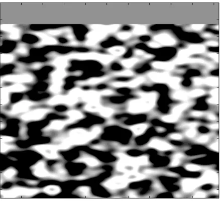
Figure 8: Random acoustic velocity model with background velocity of 3000 m/s and con-stant density of 2500 kg/m3. The medium has correlation lengtha1= 30 m in the depth (x1)

direction,a2= 90 m in the offset (x2) direction and is invariant in thex3direction.

fast and slow component. As well, the effects of dispersion due to wave induced squirt–flow can be seen in the waveforms.

4.3

Acoustic applications: sub–Fresnel zone heterogeneity

To explore the efficiency and accuracy of implementing an automated linear acoustic velocity interpolation scheme, examples are presented for a 2D stochas-tic velocity model (see Figure 8). The acousstochas-tic velocity model is defined by anisotropic random Gaussian distributed heterogeneities, having correlation lengths of 90 m laterally (in thex2direction) and 30 m vertically (or in thex1direction)

and a background velocity of 3000 m/s (the maximum velocity perturbation is on the order of±10%). The model is extended into 3D by introducing a third dimension (i.e.,x3) and is invariant with respect tox2. The random model has

dimension 2048×2048 m2 _{laterally (x}

α) and 1150 m vertically (x1). For the

examples presented, a plane–wave is extrapolated on a computational domain having 128×128 lateral grid points with 16 m spacing and x1 extrapolation

stepǫof 2 m.

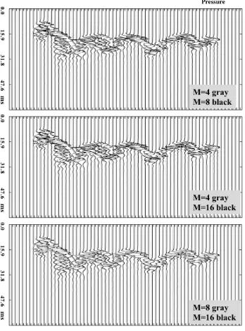
Figure 10 compares extrapolated plane–waves having a Ricker source wavelet with peak frequency of approximately 235 Hz. By lowering the source wavelet peak frequency, the effect of decreasing model interpolation on waveform fre-quency content is less pronounced. For this example, the optimum number of model interpolants is close to N=4.

The results indicate that the automated natural interpolation scheme allows sufficiently accurate computation of acoustic wavefields. For smoothly varying velocity models the scheme yields relatively identical results for both N=2 and 10 interpolants, even for large velocity perturbation [42]. The simulations indi-cate that there exists a trade–off between waveform frequency content and the number of model velocity interpolants. This suggests that when the medium is expected to vary significantly on the sub–Fresnel zone scale more interpolants are necessary to accurately simulate high frequencies. However, it should be stressed that the waveforms presented here were chosen deliberately in the high frequency range to enhance simulated wavefront and waveform distortion effects and to examine the limitations of the method for high frequency wavefields.

5

Conclusions

The one–way wave equation approach has been shown to accurately simulate the propagation of elastic waves in generally–anisotropic (for the elastic case) and smoothly varying heterogeneous, 3D media. Since the one–way propagator can be implemented in the frequency domain, I have shown also the poten-tial of modeling wave propagation in visco–elastic media, such as the case of frequency–dependent fractured media. Although the vector elastic narrow–angle wave equation is the most restrictive of all the elastic one–way wave equations derived by [36], it does allow the closest examination of the influence of the elasticity tensor on wave propagation in terms of the local directional prop-erties of the slowness surface and polarizations. Furthermore, adaptation to curvilinear coordinates can improve the narrow–angle restriction [38], increas-ing the range of allowable slownesses as well as introducincreas-ing point–sources. A key feature of the one–way approach is the ability to model gradual vector (for the narrow–angle equations) and scalar (for the acoustic wide–angle equation) waveform evolution along the underlying wavefront. This is important because the Earth displays not only vertical, but also lateral variations in heterogeneity and anisotropy. Across a dense array of receivers, the gradual evolution of the seismic wavefield is observable and the variations in the frequency dependent effects due to anisotropy and heterogeneity can be significant. The capability of modeling the evolution of these wave phenomena across an array can not only help in constraining both the vertical and lateral variations in material properties, but also highlight significant observable wave phenomena. Thus, it is expected that the one–way propagator approach will be useful for a range of transmitted wave 3D global, exploration and engineering scale applications.

extrapolator is more generally applicable than ray methods. This is primarily because it can handle robustly transitions from weak–to–strong or arbitrary anisotropy, is not limited by caustics and can model wave coupling. However, it is important to reiterate that for most problems considered in seismology, there is no one correct approach to the evaluation of the wave solution. Rather, there are various approaches available and their appropriateness depends on the required accuracy, speed and robustness of the calculated solution.

In the opinion of [104], recent advances in computer architecture will al-low 3D simulations of global seismic wave propagation on high–performance computing systems in a matter of seconds in the not so distant future. These computational advances will lead to earthquake source and tomographic inver-sions based solely on full–wave numerical methods, such as the spectral–element method [4; 105; 106]. Whether or not this view is overly optimistic, there is presently still a need for efficient, although approximate, wave solutions to con-strain hypotheses. Furthermore, algorithms that are not restricted to paral-lel computing architectures, but rather can be performed on standard desktop computers will likely still be preferred, especially for researchers with limited computational resources. It is also possible that the one–way approach will be used in the field as a preliminary modeling or processing tool.

One of the primary difficulties associated with waveform inversion is the strong non–linearity of the inverse problem. This non–linearity becomes im-portant when the medium is complicated, but is further aggravated when the data include large–offset or wide–angle data [69]. Large offset transmitted wave data are becoming increasingly prevalent because it has been recognized that they are required to resolve lateral structure [107]. In fact, a recent survey of frequency–domain waveform inversion algorithms has indicated that large off-set transmitted or refracted data are commonly applied in seismic tomographic imaging [107]. The non–linearity of the inversion can be improved by precon-ditioning the data as well as having a good starting model. These starting models are usually obtained from conventional traveltime tomography and so are limited by the asymptotic ray approximation. However, newer methods such as the so–called strongly damped wave equation can be used to compute the first–arrival traveltimes [108] or one–way wave equations to compute the most energetic traveltimes and amplitudes [54]. In theory, the acoustic wide–angle wave equation should be applicable to acoustic full–waveform inversion (and the narrow–angle wave equation for elastic full–waveform inversion) either as a means of generating a starting model or as an approximate elastic wave extrap-olator for the iterative forward and reverse propagation steps. However, the theoretical details of its implementation in waveform inversion have yet to be clarified.

Acknowledgments