This is a repository copy of
Interpreting random forest classification models using a feature
contribution method
.
White Rose Research Online URL for this paper:
http://eprints.whiterose.ac.uk/79160/
Version: Accepted Version
Book Section:
Palczewska, AM, Palczewski, J, Marchese Robinson, R et al. (1 more author) (2014)
Interpreting random forest classification models using a feature contribution method. In:
Bouabana-Tebibel, T and Rubin, SH, (eds.) Integration of Reusable Systems. Springer ,
193 - 218 (26). ISBN 3319047167
https://doi.org/10.1007/978-3-319-04717-1_9
[email protected] https://eprints.whiterose.ac.uk/
Reuse
Unless indicated otherwise, fulltext items are protected by copyright with all rights reserved. The copyright exception in section 29 of the Copyright, Designs and Patents Act 1988 allows the making of a single copy solely for the purpose of non-commercial research or private study within the limits of fair dealing. The publisher or other rights-holder may allow further reproduction and re-use of this version - refer to the White Rose Research Online record for this item. Where records identify the publisher as the copyright holder, users can verify any specific terms of use on the publisher’s website.
Takedown
If you consider content in White Rose Research Online to be in breach of UK law, please notify us by
Interpreting random forest classification models using a
feature contribution method
Anna Palczewska1
, Jan Palczewski2
, Richard Marchese Robinson3
, and Daniel Neagu1
1
Department of Computing, University of Bradford, BD7 1DP Bradford, UK,
[email protected], [email protected]
2
School of Mathematics, University of Leeds, LS2 9JT Leeds, UK,
3
School of Pharmacy and Biomolecular Sciences, Liverpool John Moores University, L3 3AF Liverpool, UK,
Abstract. Model interpretation is one of the key aspects of the model evaluation process. The explanation of the relationship between model variables and out-puts is relatively easy for statistical models, such as linear regressions, thanks to the availability of model parameters and their statistical significance. For “black box” models, such as random forest, this information is hidden inside the model structure. This work presents an approach for computing feature contributions for random forest classification models. It allows for the determination of the influ-ence of each variable on the model prediction for an individual instance and an additional assessment of model reliability for new data. Interpretation of feature contributions for two UCI benchmark datasets shows the potential of the pro-posed methodology. The robustness of results is demonstrated through an exten-sive analysis of feature contributions calculated for a large number of generated random forest models.
1
Introduction
Models are used to discover interesting patterns in data or to predict a specific outcome, such as drug toxicity, client shopping purchases, or car insurance premium. They are often used to support human decisions in various business strategies. This is why it is important to ensure model quality and to understand its outcomes. Good practice of model development [17] involves: 1) data analysis 2) feature selection, 3) model building and 4) model evaluation. Implementing these steps together with capturing information on how the data was harvested, how the model was built and how the model was validated, allows us to trust that the model gives reliable predictions. But, how to interpret an existing model? How to analyse the relation between predicted values and the training dataset? Or which features contribute the most to classify a specific instance?
However, in the recent literature, there has been considerable focus on interpreting pre-dictions made by non-linear models which do not render themselves to straightforward methods for the determination of variable/feature influence. In [8], the authors present a method for a local interpretation of Support Vector Machine (SVM) and Random Forest model by retrieving the variable corresponding to the largest component of the decision-function gradient at any point in the model. Interpretation of classification models using local gradients is discussed in [4]. A method for visual interpretation of kernel-based prediction models is described in [11]. Another approach, which is presented in detail later, was proposed in [12] and aims at shedding light at decision-making process of regression random forests.
Of interest to this paper is a popular “black-box” model – the random forest model [5]. Its author suggests two measures of the significance of a particular variable [6]: the variable importance and the Gini importance. The variable importance is derived from the loss of accuracy of model predictions when values of one variable are permuted be-tween instances. Gini importance is calculated from the Gini impurity criterion used in the growing of trees in the random forest. However, in [16], the authors showed that the above measures are biased in favor of continuous variables and variables with many cat-egories what do not allow for a thorough analysis of a model. They also demonstrated that the general representation of variable importance is often insufficient for the com-plete understanding of the relationship between input variables and the predicted value. Following the above observation, Kuzmin et al. propose in [12] a new technique to calculate the feature contribution, i.e., the contribution of a variable to the predic-tion, in a random forest model with numerical observed values (the observed value is a real number). Unlike in the variable importance measures [6], feature contributions are computed separately for each instance/record and provide detailed information about relationships between variables and the predicted value: the extent and the kind of in-fluence (positive/negative) of a given variable. This new approach was positively tested in [12] on a Quantitative Structure-Activity (QSAR) model for chemical compounds. The results were not only informative about the structure of the model but also provided valuable information for the design of new compounds.
The procedure from [12] for the computation of feature contributions applies to random forest models predicting numerical observed values. This paper aims to extend it to random forest models with categorical predictions, i.e., where the observed value determines one from a finite set of classes. The difficulty of achieving this aim lies in the fact that a discrete set of classes does not have the algebraic structure of real numbers which the approach presented in [12] relies on. Due to the high-dimensionality of the calculated feature contributions, their direct analysis is not easy. We develop three techniques for discovering patterns in the decision-making process of random forest models. This facilitates interpretation of model predictions as well as allows a more detailed analysis of model’s reliability for an unseen data.
the proposed methodology to two real world datasets from the UCI Machine Learning repository. Section 7 concludes the work presented in this paper.
2
Random Forest
A random forest (RF) model introduced by Breiman [5] is a collection of tree predictors. Each tree is grown according to the following procedure [6]:
1. the bootstrap phase: select randomly a subset of the training dataset – a local train-ing set for growtrain-ing the tree. The remaintrain-ing samples in the traintrain-ing dataset form a so-called out-of-bag (OOB) set and are used to estimate the RF’s goodness-of-fit. 2. the growing phase: grow the tree by splitting the local training set at each node
according to the value of one from a randomly selected subset of variables (the best split) using classification and regression tree (CART) method [7].
3. each tree is grown to the largest extent possible. There is no pruning.
The bootstrap and the growing phases require an input of random quantities. It is as-sumed that these quantities are independent between trees and identically distributed. Consequently, each tree can be viewed as sampled independently from the ensemble of all tree predictors for a given training dataset.
For prediction, an instance is run through each tree in a forest down to a terminal node which assigns it a class. Predictions supplied by the trees undergo a voting pro-cess: the forest returns a class with the maximum number of votes. Draws are resolved through a random selection.
To present our feature contribution procedure in the following section, we have to develop a probabilistic interpretation of the forest prediction process. Denote byC =
{C1, C2, . . . , CK}the set of classes and by∆Kthe set
∆K =
(p1, . . . , pK) :
K
X
k=1
pk = 1andpk≥0 .
An element of∆Kcan be interpreted as a probability distribution overC. Letekbe an
element of∆Kwith1at positionk– a probability distribution concentrated at classCk.
If a treetpredicts that an instanceibelongs to a classCkthen we writeYˆi,t=ek. This
provides a mapping from predictions of a tree to the set∆Kof probability measures on
C. Let
ˆ
Yi=
1
T
T
X
t=1
ˆ
Yi,t, (1)
whereTis the overall number of trees in the forest. ThenYˆi ∈∆Kand the prediction
of the random forest for the instancei coincides with a classCk for which thek-th
coordinate ofYˆiis maximal.4
4
The distributionYˆiis calculated by the functionpredictin the R packagerandomForest
3
Feature Contributions for Binary Classifiers
The set∆K simplifies considerably when there are two classes, K = 2. An element
p∈∆K is uniquely represented by its first coordinatep1(p2= 1−p1). Consequently,
the set of probability distributions onCis equivalent to the probability weight assigned to classC1.
Before we can present our method for computing feature contributions, we have to examine the tree growing process. After selecting a training set, it is positioned in the root node. A splitting variable (feature) and a splitting value are selected and the set of instances is split between the left and the right child of the root node. The procedure is repeated until all instances in a node are in the same class or further splitting does not improve prediction. The class that a tree assigns to a terminal node is determined through majority voting between instances in that node.
We will refer to instances of the local training set that pass through a given node as the training instances in this node. The fraction of the training instances in a noden
belonging to classC1will be denoted byYmeann . This is the probability that a randomly
selected element from the training instances in this node is in the first class. In particular, a terminal node is assigned to classC1ifYmeann >0.5orYmeann = 0.5and the draw is
resolved in favor of classC1.
The feature contribution procedure for a given instance involves two steps: 1) the calculation of local increments of feature contributions for each tree and 2) the aggre-gation of feature contributions over the forest. A local increment corresponding to a featuref between a parent node (p) and a child node (c) in a tree is defined as follows:
LIfc =
Yc
mean−Y p mean,
if the split in the parent is performed over the featuref,
0, otherwise.
A local increment for a featuref represents the change of the probability of being in class C1 between the child node and its parent node provided that f is the splitting
feature in the parent node. It is easy to show that the sum of these changes, over all features, along the path followed by an instance from the root node to the terminal node in a tree is equal to the difference betweenYmeanin the terminal and the root node.
The contributionF Ci,tf of a featurefin a treetfor an instanceiis equal to the sum
ofLIf over all nodes on the path of instanceifrom the root node to a terminal node.
The contribution of a featuref for an instanceiin the forest is then given by
F Cif =
1
T
T
X
t=1
F Ci,tf . (2)
The feature contributions vector for an instanceiconsists of contributionsF Cif of all
featuresf.
Notice that if the following condition is satisfied:
thenYˆirepresenting forest’s prediction (1) can be written as
ˆ
Yi=
Yr+X
f
F Cif, 1−Y
r−X f
F Cif
(3)
whereYr
is the coordinate-wise average ofYmeanover all root nodes in the forest. If
this unanimity condition (U) holds, feature contributions can be used to retrieve predic-tions of the forest. Otherwise, they only allow for the interpretation of the model.
3.1 Example
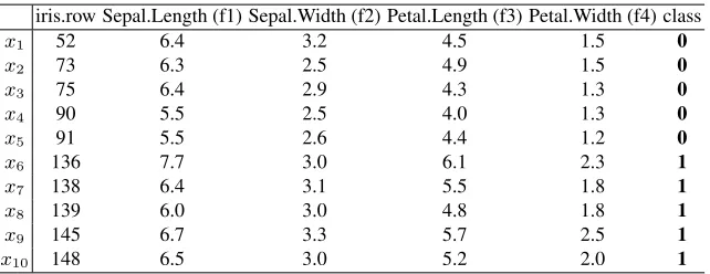
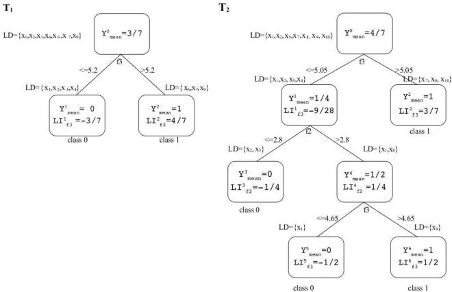
We will demonstrate the calculation of feature contributions on a toy example using a subset of the UCI Iris Dataset [3]. From the original dataset, ten records were selected – five for each of two types of the iris plant: versicolor (class 0) and virginica (class 1) (see Table 1). A plant is represented by four attributes: Sepal.Length (f1), Sepal.Width (f2), Petal.Length (f3) and Petal.Width (f4). This dataset was used to generate a random forest model with two trees, see Figure 1. In each tree, the local training set (LD) in the root node collects those records which were chosen by the random forest algorithm to build that tree. The LD sets in the child nodes correspond to the split of the above set according to the value of a selected feature (it is written between branches). This process is repeated until reaching terminal nodes of the tree. Notice that the condition
[image:6.612.149.470.446.570.2](U)is satisfied – for both trees, each terminal node contains local training instances of the same class:Ymeanis either0or1.
Table 1: Selected records from the UCI Iris Dataset. Each record corresponds to a plant. The plants were classified as iris versicolor (class 0) and virginica (class 1).
iris.row Sepal.Length (f1) Sepal.Width (f2) Petal.Length (f3) Petal.Width (f4) class
x1 52 6.4 3.2 4.5 1.5 0
x2 73 6.3 2.5 4.9 1.5 0
x3 75 6.4 2.9 4.3 1.3 0
x4 90 5.5 2.5 4.0 1.3 0
x5 91 5.5 2.6 4.4 1.2 0
x6 136 7.7 3.0 6.1 2.3 1
x7 138 6.4 3.1 5.5 1.8 1
x8 139 6.0 3.0 4.8 1.8 1
x9 145 6.7 3.3 5.7 2.5 1
x10 148 6.5 3.0 5.2 2.0 1
The process of calculating feature contributions runs in 2 steps: the determination of local increments for each node in the forest (a preprocessing step) and the calculation of feature contributions for a particular instance. Figure 1 showsYn
mean and the local
incrementLIc
ffor a splitting featurefin each node. Having computed these values, we
Fig. 1: A random forest model for the dataset from Table 1. The set LD in the root node contains a local training set for the tree. The sets LD in the child nodes correspond to the split of the above set according to the value of selected feature. In each node,Yn
mean denotes the fraction
of instances in the LD set in this node belonging to class 1, whilstLIn
f shows non-zero local
increments.
a given feature for the instancex1is calculated by summing local increments for that
feature along the pathp1 =n0→n1in treeT1and the pathp2 =n0→n1→n4→
n5in treeT2. According to Formula (2) the contribution of feature f2 is calculated as
F Cf2
x1 =
1 2
0 + 1 4
= 0.125
and the contribution of feature f3 is
F Cf3
x1 =
1 2
−3
7 − 9 28−
1 2
=−0.625.
The contributions of features f1 and f4 are equal to0because these attributes are not used in any decision made by the forest. The predicted probabilityYˆx1 thatx1belongs
to class 1 (see Formula (3)) is
ˆ
Yx1 =
1 2
3
7 + 4 7
| {z }
ˆ Yr
+ 0 + 0.125−0.625 + 0
| {z }
P fF C
f x1
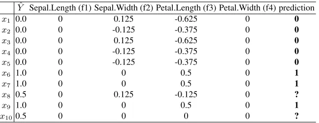
[image:7.612.139.469.125.338.2]= 0.0
Table 2: Feature contributions for the random forest model from Figure 1.
ˆ
Y Sepal.Length (f1) Sepal.Width (f2) Petal.Length (f3) Petal.Width (f4) prediction
x1 0.0 0 0.125 -0.625 0 0
x2 0.0 0 -0.125 -0.375 0 0
x3 0.0 0 0.125 -0.625 0 0
x4 0.0 0 -0.125 -0.375 0 0
x5 0.0 0 -0.125 -0.375 0 0
x6 1.0 0 0 0.5 0 1
x7 1.0 0 0 0.5 0 1
x8 0.5 0 0.125 -0.125 0 ?
x9 1.0 0 0 0.5 0 1
x100.5 0 0 0 0 ?
– for instancesx1, x3, the contribution of f2 is positive, i.e., the value of this feature
increases the probability of being in class 1 by 0.125. However, the large negative contribution of the feature f3 implies that the value of this feature for instancesx1
andx3was decisive in assigning the class 0 by the forest.
– for instancesx6, x7, x9, the decision is based only on the feature f3.
– for instancesx2, x4, x5, the contribution of both features leads the forest decision
towards class 0.
– for instancesx8,x10,Yˆ is0.5. This corresponds to the case where one of the trees
points to class 0 and the other to class 1. In practical applications, such situations are resolved through a random selection of the class. SinceYˆr = 0.5, the lack of
decision of the forest has a clear interpretation in terms of feature contributions: the amount of evidence in favour of one class is counterbalanced by the evidence pointing towards the other.
4
Feature Contributions for General Classifiers
WhenK > 2, the set∆K cannot be described by a one-dimensional value as above.
We, therefore, generalize the quantities introduced in the previous section to a multi-dimensional case. Yn
mean in a noden is an element of∆K, whose k-th coordinate,
k= 1,2, . . . , K, is defined as
Ymean,kn =
|{i∈T S(n) : i∈Ck}|
|T S(n)| , (4)
whereT S(n)is the set of training instances in the nodenand| · |denotes the number of elements of a set. Hence, if an instance is selected randomly from a local training set in a noden, the probability that this instance is in class Ck is given by thek-th
coordinate of the vectorYn
multidimensional case:
LIfc =
Yc
mean−Ymeanp ,
if the split in the parent is performed over the featuref,
(0, . . . ,0)
| {z }
Ktimes
, otherwise,
where the difference is computed coordinate-wise. Similarly,F Ci,tf andF C f i are
ex-tended to vector-valued quantities. Notice that if the condition (U) is satisfied, Equation (3) holds withYr
being a coordinate-wise average of vectorsYn
meanover all root nodes
nin the forest.
Fix an instanceiand letCk be the class to which the forest assigns this instance.
Our aim is to understand which variables/features drove the forest to make that predic-tion. We argue that the crucial information is that which explains the value of thek-th coordinate ofYˆi. Hence, we want to study thek-th coordinate ofF C
f
i for all features
f.
Pseudo-code to calculate feature contributions for a particular instance towards the class predicted by the random forest is presented in Algorithm 1. Its inputs consist of a random forest modelRF and an instancei which is represented as a vector of feature values. In line 1,k ∈ {1,2, . . . , K}is assigned the index of a class predicted by the random forest RF for the instancei. The following line creates a vector of real numbers indexed by features and initialized to0. Then for each tree in the forestRF
the instanceiis run down the tree and feature contributions are calculated. The quantity
SplitF eature(parent) identifies a featuref on which the split is performed in the
nodeparent. If the valuei(f)of that featureffor the instanceiis lower or equal to the
thresholdSplitV alue(parent), the route continues to the left child of the nodeparent. Otherwise, it goes to the right child (each node in the tree has either two children or is a terminal node). A position corresponding to the featuref in the vectorF Cis updated according to the change of value ofYmean,k, i.e., thek-th coordinate ofYmean, between
the parent and the child.
Algorithm 2 provides a sketch of the preprocessing step to computeYn
meanfor all
nodesnin the forest. The parameterD denotes the set of instances used for training of the forestRF. In line 2,T Sis assigned the set used for growing treeT. This set is further split in nodes according to values of splitting variables. We propose to use DFS (depth first search [9]) to traverse the tree and compute the vectorYn
meanonce a training
set for a nodenis determined. There is no need to store a training set for a nodenonce
Yn
meanhas been calculated.
5
Analysis of Feature Contributions
Algorithm 1FC(RF,i)
1: k←f orest predict(RF, i)
2: F C←vector(f eatures)
3: foreach treeTin forestFdo
4: parent←root(T)
5: whileparent! = TERMINALdo
6: f←SplitF eature(parent)
7: ifi[f]<=SplitV alue(parent)then
8: child←lef tChild(parent)
9: else
10: child←rightChild(parent)
11: end if
12: F C[f]←F C[f] +Ymean,kchild −Yparent
mean,k
13: parent←child
14: end while
15: end for
16: F C←F C/ nTrees(F)
17: return F C
Algorithm 2Ymean(RF, D) 1: foreach treeTin forestFdo
2: T S←training set for treeT
3: use DFS algorithm to compute training sets in all other nodesnof treeT and compute the vectorYn
meanaccording to formula (4).
4: end for
predictions for unseen instances. They provide complementary information to forest’s voting results. This section proposes three techniques for finding patterns in the way a random forest uses available features and linking these patterns with the forest’s predic-tions.
5.1 Median
If most of instances from the training dataset belonging to a particular class is close to the corresponding vector of medians, we may treat this vector justifiably as a standard level. When a prediction is requested for a new instance, we query the random forest model for the fraction of trees voting for each class and calculate feature contributions leading to its final prediction. If a high fraction of trees votes for a given class and the feature contributions are close to the standard level for this class, we may reasonably rely on the prediction. Otherwise we may doubt the random forest model prediction.
It may, however, happen that many instances from the training dataset correctly predicted to belong to a particular class are distant from the corresponding vector of medians. This might suggest that there is more than one standard level, i.e., there might be multiple mechanisms relating the features to the correct class such that the feature contributions could vary significantly from the median yet still not indicate the corre-sponding predictions are unreliable. The next subsection presents more advanced meth-ods capable of finding a number of standard levels – distinct patterns followed by the random forest model in its prediction process.
5.2 Cluster Analysis
Clustering is an approach for grouping elements/objects according to their similarity [10]. This allows us to discover patterns that are characteristic for a particular group. As we discussed above, feature contributions in one class may have more than one ”standard level”. When this is discovered, clustering techniques can be employed to find if there is a small number of distinct standard levels, i.e., feature contributions of the instances in the training dataset group around these points with only a relatively few instances being far away from them; these few instances are then treated as unusual representatives of a given class. We shall refer to clusters of instances around these standard levels as ”core clusters”.
The analysis of core clusters can be of particular importance for applications. For example, in the classification of chemical compounds, the split into clusters may point to groups of compounds with different mechanisms of activity. We should note that the similarity of feature contributions does not imply that particular features are similar. We examined several examples and noticed that clustering based upon the feature values did not yield useful results whereas the same method applied to feature contributions was able to determine a small number of core clusters.
RF Model
Training Data
Feature Contributions
f11, f12, …,f1n
. . . . .
fm1, fm2, ..., f
mn
New instance
Predictions
f1, f2, ..., fn
Decision
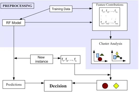
[image:12.612.165.450.138.329.2]Cluster Analysis PREPROCESSING
Fig. 2: The workflow for assessing the reliability of the prediction made by a random forest (RF) model.
at the structure and performance of the resulting clusters: for each cluster we assess the average fraction of trees voting for the predicted class across the instances belonging to this cluster as well as the average distance from the centre of the cluster. Relatively large clusters with the former value close to1and the latter value small form the group of core clusters.
To assess the reliability of the model prediction for a new instance, we recommend looking at two measures: the fraction of trees voting for the predicted class as well as the cluster to which the instance is assigned based on its feature contributions. If the cluster is one of the core clusters and the distance from its center is relatively small, the instance is a typical representative of its predicted class. This together with high decisiveness of the forest suggests that the model’s prediction should be trusted. Otherwise, we should allow for an increased chance of misclassification.
5.3 Log-likelihood
fea-F1 F2 F3 F4
−0.10
0.00
0.10
0.20
Feature
F
eature contr
ib
[image:13.612.205.390.151.313.2]ution
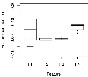
Fig. 3: The boxplot for feature contributions within a core cluster for a hypothetical random forest model.
tures are stable within a cluster – the height of the box is small. Others (F1 and F4) display higher variability. One would therefore expect that the same divergence of con-tributions for features F3 and F4 from their mean value should be treated differently. It is more significant for the feature F3 than for the feature F4. This is unfortunately not taken into account when the Euclidean distance is considered. Here, we propose an alternative method for assessing the distance from the cluster centre which takes into account the variation of feature contributions within a cluster. Our method has proba-bilistic roots and we shall present it first from a statistical point of view and provide other interpretations afterwards.
We assume that feature contributions for instances within a cluster share the same base values(µf)- the centre of the cluster. We attribute all discrepancies between this
base value and the actual feature contributions to a random perturbation. These per-turbations are assumed to be normally distributed with the mean 0 and the variance
σ2
f, where f denotes the feature. The variance of the perturbation for each feature is
selected separately – we use the sample variance computed from feature contributions of instances of the training dataset belonging to this cluster. Although it is clear that perturbations for different features exhibit some dependence, it is impossible to assess it given the numer of instances in a cluster and a large number of features typically in use.5Therefore, we resort to a common solution: we assume that the dependence be-tween perturbations is small enough to justify treating them as independent.
Summaris-5A covariance matrix of feature contribution hasF(F+ 1)/2distinct entries, whereF is the
Ap-ing, our statistical model for the distribution of feature contributions within a cluster is as follows: feature contributions for instances within a cluster are composed of a base value and a random perturbation which is normally distributed and independent between features.
Take an instanceiwith feature contributionsF Cif. The log-likelihood of being in a
cluster with the center(µf)and variances of perturbations(σ2f)is given by
LLi=
X
f
−(F C
f i −µf)2
2σ2 f
−1
2log(2πσ
2 f)
. (5)
The higher the log-likelihood the bigger the chance of feature contributions of the in-stanceito belong to the cluster. Notice that the above sum takes into account the obser-vations we made at the beginning of this subsection. Indeed, as the second term in the sum above is independent of the considered instance, the log-likelihood is equivalent to
X
f
−(F C
f i −µf)
2
2σ2 f
,
which is the negative of the squared weighted Euclidean distance betweenF Cif and
µf with the weights being inversely proportional to the variability of a given feature
contribution in the training instances in the cluster. In our toy example of Figure 3, this corresponds to penalizing more for discrepancies for features F2 and F3, and signifi-cantly less for discrepancies for features F1 and F4.
In the following section, we analyse relations between the log-likelihood and clas-sification for a UCI Breast Cancer Wisconsin Dataset.
6
Applications
In this section, we demonstrate how the techniques from the previous section can be applied to improve understanding of a random forest model. We consider one example of a binary classifier using the UCI Breast Cancer Wisconsin Dataset [1] (BCW Dataset) and one example of a general classifier for the UCI Iris Dataset [3]. We complement our studies with a robustness analysis.
6.1 Breast Cancer Wisconsin Dataset
The UCI Breast Cancer Wisconsin Dataset contains characteristics of cell nuclei for 569 breast tissue samples; 357 are diagnosed as benign and 212 as malignant. The characteristics were captured from a digitized image of a fine needle aspirate (FNA) of a breast mass. There are 30 features, three (the mean, the standard error and the average of the three largest values) for each of the following 10 characteristics: radius, texture, perimeter, area, smoothness, compactness, concavity, concave points, symmetry and
F2 F5 F7 F14 F17 F22 F25 F28 F30
Features
F
eature contr
ib
ution
−0.05
0.00
0.05
0.10
[image:15.612.188.410.134.279.2]0.15
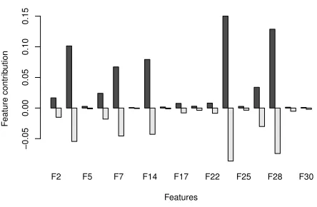
Fig. 4: Medians of feature contributions for each class for the BCW Dataset. The light grey bars represent contributions toward class 1 and the black bars show contributions towards class 0.
fractal dimension. For brevity, we numbered these features fromF1toF30according to their order in the data file.
To reduce correlation between features and facilitate model interpretation, the min-max (minimal-redundancy-min-maximal-relevance) method was applied and the following features were removed from the dataset: 1, 3, 8, 10, 11, 13, 12, 15, 19, 10, 21, 24, 26. A random forest model was generated on 2/3 randomly selected instances using 500 trees. The other 1/3 of instances formed the testing dataset. The test set validation showed that the model accuracy was 0.9682 (only 6 instances out of 189 were classified incorrectly); similar accuracy was achieved when the model was generated using all the features.
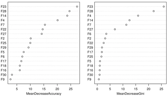
We applied our feature contribution algorithm to the above random forest binary classifier. To align notation with the rest of the paper, we denote the class “malignant” by 1 and the class “benign” by 0. Aggregate results for the feature contributions for all training instances and both classes are presented in Figure 4. Light-grey bars show medians of contributions for instances of class 1 (malignant), whereas black bars show medians of contributions for instances of class 0. Notice that there are only a few sig-nificant features in the graph: F4 – the mean of the cell area, F7 – the mean of the cell concavity, F14 – the standard deviation of the cell area, F23 – the average of three largest measurements of the cell perimeter and F28 – the average of three largest measurements of concave points. This selection of significant features is perfectly in agreement with the results of the permutation based variable importance (the left panel of Figure 5) and the Gini importance (the right panel of Figure 5). Interpreting the size of bars as the level of importance of a feature, our results are in line with those provided by the Gini index. However, the main advantage of the approach presented in this paper lies in the fact that one can study the reasons for the forest’s decision for aparticular instance.
F9 F30 F16 F18 F17 F6 F5 F29 F25 F2 F27 F22 F7 F4 F14 F28 F23
5 10 15 20 25 MeanDecreaseAccuracy
F9 F30 F16 F18 F5 F25 F17 F29 F22 F2 F6 F27 F7 F14 F4 F28 F23
0 5 10 15 20 25
MeanDecreaseGini
[image:16.612.141.476.158.349.2]breastrfmtest
Fig. 5: The left panel shows permutation based variable importance and the right panel displays Gini importance for a RF binary classification model developed for the BCW Dataset. Graphs generated using randomForest package in R.
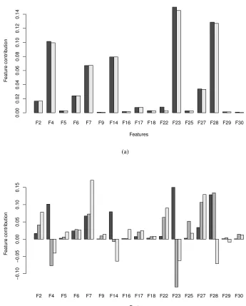
the large majority of trees votes for class 1 the feature contributions for that instance are very close to the median values (see Figure 6a). This happens for around80%of all instances from the testing dataset predicted to be in class 1. However, when the decision is less unanimous, the analysis of feature contributions may reveal interesting informa-tion. As an example, we have chosen instances 194 and 537 (see Table 3) which were classified correctly as malignant (class 1) by a majority of trees but with a significant number of trees expressing an opposite view. Figure 6b presents feature contributions for these two instances (grey and light grey bars) against the median values for class 1 (black bars). The largest difference can be seen for the contributions of very significant features F23, F4 and F14: it is highly negative for the two instances under consideration compared to a large positive value commonly found in instances of class 1. Recall that
Table 3: Percentage of trees that vote for each class in RF model for a selection of instances from the BCW Dataset.
Instance Id benign (class 0) malignant (class 1)
3 0 1
194 0.298 0.702
F2 F4 F5 F6 F7 F9 F14 F16 F17 F18 F22 F23 F25 F27 F28 F29 F30
Features
F
eature contr
ib
ution
0.00
0.02
0.04
0.06
0.08
0.10
0.12
0.14
(a)
F2 F4 F5 F6 F7 F9 F14 F16 F17 F18 F22 F23 F25 F27 F28 F29 F30
Features
F
eature contr
ib
ution
−0.10
−0.05
0.00
0.05
0.10
0.15
[image:17.612.132.477.139.568.2](b)
a negative value contributes towards the classification in class 0. There are also three new significant attributes (F2, F22 and F27) that contribute towards the correct classifi-cation as well as unusual contributions for features F7 and F28. These newly significant features are judged as only moderately important by both of the variable importance methods in Figure 5. It is, therefore, surprising to note that the contribution of these three new features was instrumental in correctly classifying instances 194 and 537 as malignant. This highlights the fact that features which may not generally be important for the model may, nonetheless, be important for classifying specific instances. The approach presented in this paper is able to identify such features, whilst the standard variable importance measures for random forest cannot.
6.2 Cluster Analysis and Likelihood Ratio
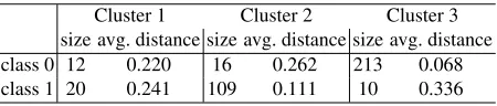
[image:18.612.196.421.453.501.2]The training dataset previously derived for the BCW Dataset was partitioned according to the true class labels. A clustering algorithm implemented in the R package kmeans was run separately for each class. This resulted in the determination of three clusters for class 0 and three clusters for class 1. The structure and size of clusters is presented in Table 4. Each class has one large cluster: cluster 3 for class 0 and cluster 2 for class 1. Both have a bigger concentration of points around the cluster center (small average distance) than the remaining clusters. This suggests that there is exactly one core cluster corresponding to a class. This explains the success of the analysis based on the median as the vectors of medians are close to the centers of unique core clusters.
Table 4: The structure of clusters for BCW Dataset. For each cluster, the size (the number of training instances) is reported in the left column and the average Euclidean distance from the cluster center among the training dataset instances belonging to this cluster is displayed in the right column.
Cluster 1 Cluster 2 Cluster 3 size avg. distance size avg. distance size avg. distance class 0 12 0.220 16 0.262 213 0.068 class 1 20 0.241 109 0.111 10 0.336
1 2 3
0.75
0.80
0.85
0.90
0.95
1.00
Cluster
Probability of class 0
(a) Class 0
1 2 3
0.7
0.8
0.9
1.0
Cluster
Probability of class 1
[image:19.612.152.453.143.308.2](b) Class 1
Fig. 7: Fraction of forest trees voting for the correct class in each cluster for training part of the BCW Dataset.
F2 F4 F5 F6 F7 F9 F14 F16 F17 F18 F22F23 F25 F27 F28F29 F30
−0.2
−0.1
0.0
0.1
0.2
0.3
Feature
F
eature contr
ib
ution
Cluster 1
F2 F4 F5 F6 F7 F9 F14 F16F17 F18 F22 F23 F25F27 F28 F29 F30
−0.2
−0.1
0.0
0.1
0.2
0.3
Feature
F
eature contr
ib
ution
Cluster 2
F2 F4 F5 F6 F7 F9 F14 F16 F17 F18F22 F23 F25 F27F28 F29 F30
−0.2
−0.1
0.0
0.1
0.2
0.3
Feature
F
eature contr
ib
ution
Cluster 3
[image:19.612.140.470.365.623.2]−250 −200 −150 −100 −50 0 50 100
−500
−400
−300
−200
−100
0
100
Log−likelihood for the core cluster in class 1
Log−lik
elihood f
[image:20.612.169.432.140.318.2]or the core cluster in class 0
Fig. 9: Loglikelihoods for belonging to the core cluster in class 0 (vertical axis) and class 1 (hor-izontal axis) for the testing dataset in BCW. Red circles correspond to instances of class 0 while blue circles denote instances of class 1.
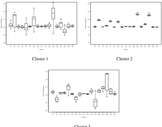
similarity of instances (in terms of their feature contributions) in the core class. One can see much higher variability in two remaining clusters showing that the forest used different features as evidence to classify instances in each of these clusters. Although in cluster 2 all contributions were positive, in clusters 1 and 3 there are features with negative contributions. Recall that a negative value of a feature contribution provides evidence against being in the corresponding class, here class 1.
Based on the observation that clusters correspond to a particular decision-making route for the random forest model, we introduced the loglikelihood as a way to assess the distance of a given instance from the cluster centre, or, in a probabilistic interpreta-tion, to compute the likelihood6that the instance belongs to the given cluster. It should
however be clarified that one cannot compare the likelihood for the core cluster in class 0 with the likelihood for the core cluster in class 1. The likelihood can only be used for comparisons within one cluster: having two instances we can say which one is more likely to belong to a given cluster. By comparing it to a typical likelihood for training instances in a given cluster we can further draw conclusions about how well an instance fits that cluster. Figure 9 presents the loglikelihoods for the two core clusters (one for each class) for instances from the testing dataset. Colors are used to mark instances belonging to each class: red for class 0 and blue for class 1. Notice that likelihoods provide a very good split between classes: instances belonging to class 0 have a high
loglikelihood for the core cluster of class 0 and rather low loglikelihood for the core cluster of class 1. And vice-versa for instances of class 1.
6.3 Iris Dataset
In this section we use the UCI Iris Dataset [3] to demonstrate interpretability of feature contributions for multi-classification models. We generated a random forest model on 100 randomly selected instances. The remaining 50 instances were used to assess the accuracy of the model: 47 out of 50 instances were correctly classified. Then we ap-plied our approach for determining the feature contributions for the generated model. Figure 10 presents medians of feature contributions for each of the three classes. In con-trast to the binary classification case, the medians are positive for all classes. A positive feature contribution for a given class means that the value of this feature directs the forest towards assigning this class. A negative value points towards the other classes.
Sepal.Length Sepal.Width Petal.Length Petal.Width Setosa
Versicolour Virginica
Feature
F
eature contr
ib
ution
0.00
0.05
0.10
0.15
0.20
0.25
0.30
[image:21.612.192.409.323.470.2]0.35
Fig. 10: Medians of feature contributions for each class for the UCI Iris Dataset.
Table 5: Feature contributions towards predicted classes for selected instances from the UCI Iris Dataset.
Instance Sepal Petal Length Width Length Width 120 0.059 0.014 0.053 0.448 150 -0.097 0.035 0.259 0.339
1 (Sepal.Length) which points towards a different class. In contrast, the instance 120 shows standard (low) contributions of the first two features and unusual contributions of the last two features: very low for feature 3 and high for feature 4. Recalling that features 3 and 4 tend to contribute most to the forest’s decision (see Figure 10) with values between 0.25 and 0.35, the low value for feature 3 is non-standard for its pre-dicted class, which increases the chance of it being wrongly classified. Indeed, both instances belong to class Virginica while the forest classified the instance 120 wrongly as class Versicolour and the instance 150 correctly as class Virginica.
The cluster analysis of feature contributions for the UCI Iris Dataset revealed that it is sufficient to consider only two clusters for each class. Cluster sizes are5and45for class Setosa,4and46for class Versicolour and5and44for class Virginica. Core clus-ters were straighforward to determine. Figure 11 displays an analysis of log-likelihoods for all instances in the dataset. For every instance, we computed feature contributions towards each class and calculated log-likelihoods of being in the core clusters of the respective classes. On the graph, each point represents one instance. The coordinate LH1 is the log-likelihood for the core cluster of class Setosa, the coordinate LH2 is the log-likelihood for the core cluster of class Versicolour and the coordinate LH3 is the log-likelihood for the core cluster of class Virginica. Colors of points show the true classification: class Setosa is represented by the red dots, Versicolour by the blue dots and Virginica by the green dots. Notice that points corresponding to instances of the same class tend to group together. This can be interpreted as the existence of coherent patterns in the reasoning of the random forest model.
6.4 Robustness Analysis
For the validity of the study of feature contributions, it is crucial that the results are not artefacts of one particular realization of a random forest model but that they con-vey actual information held by the data. We therefore propose a method for robustness analysis of feature contributions. We will use the UCI Breast Cancer Wisconsin Dataset studied in Subsection 6.1 as an example.
We removed instance number 3 from the original dataset to allow us to perform tests with an unseen instance. We generated 100 random forest models with 500 trees with each model built using an independent randomly generated training set with379≈
Fig. 11: Log-likelihoods for all instances in UCI Iris Dataset towards core clusters for each class.
is the25%quantile, while the bold line in the middle is the median (recalling that this is the median of the median feature contributions across multiple models). Whiskers show the extent of minimal and maximal values for each feature contribution. Notice that the variation between simulations is moderate and conclusions drawn for one realization of the random forest model in Subsection 6.1 would hold for each of the generated 100 random forest models.
F2 F4 F5 F6 F7 F9 F14 F16 F17 F18 F22 F23 F25 F27 F28 F29 F30
0.00
0.05
0.10
0.15
Feature
F
eature contr
ib
ution
(a) Medians of feature contributions for training datasets
F2 F4 F5 F6 F7 F9 F14 F16 F17 F18 F22 F23 F25 F27 F28 F29 F30
0.00
0.05
0.10
0.15
Feature
F
eature contr
ib
ution
(b) Medians of feature contributions for testing datasets
F2 F4 F5 F6 F7 F9 F14 F16 F17 F18 F22 F23 F25 F27 F28 F29 F30
0.00
0.05
0.10
0.15
Feature
F
eature contr
ib
ution
[image:24.612.193.416.134.279.2](c) Feature contributions for an unseen instance
7
Conclusions
Feature contributions provide a novel approach towards black-box model interpretation. They measure the influence of variables/features on the prediction outcome and provide explanations as to why a model makes a particular decision. In this work, we extended the feature contribution method of [12] to random forest classification models and we proposed three techniques (median, cluster analysis and log-likelihood) for finding pat-terns in the random forest’s use of available features. Using UCI benchmark datasets we showed the robustness of the proposed methodology. We also demonstrated how feature contributions can be applied to understand the dependence between instance character-istics and their predicted classification and to assess the reliability of the prediction. The relation between feature contributions and standard variable importance measures was also investigated. The software used in the empirical analysis was implemented in R as an add-on for therandomForestpackage and is currently being prepared for submission to CRAN [2] under the namerfFC.
Acknowledgements.This work is partially supported by BBSRC and Syngenta Ltd through the Industrial CASE Studentship Grant (No. BB/H530854/1).
References
1. Breast Cancer Wisconsin Diagnostic dataset.http://archive.ics.uci.edu/ml/ datasets/Breast+Cancer+Wisconsin+\%28Diagnostic\%29
2. CRAN - The Comprehensive R Archive Network.http://cran.r-project.org/
3. Iris dataset.http://archive.ics.uci.edu/ml/datasets/Iris
4. Baehrens, D., Schroeter, T., Harmeling, S., Kawanabe, M., Hansen, K., Muller, K.R.: How to explain individual classification decisions. Journal of Machine Learning Research 11, 1803– 1831 (2010)
5. Breiman, L.: Random forests. Machine Learning 45(1), 5–32 (2001)
6. Breiman, L., Cutler, A.: Random forests. http://www.stat.berkeley.edu/
˜breiman/RandomForests/(2008)
7. Breiman, L., Friedman, J.H., Olshen, R.A., Stone, C.J.: Classification and regression trees. Monterey, CA: Wadsworth & Brooks/Cole Advanced Books & Software (1984)
8. Carlsson, L., Helgee, E.A., Boyer, S.: Interpretation of nonlinear qsar models applied to ames mutagenicity data. Journal of Chemical Information and Modeling 49(11), 2551–2558 (2009)
9. Cormen, T.H., Stein, C., Rivest, R.L., Leiserson, C.E.: Introduction to Algorithms. McGraw-Hill Higher Education, 2nd edn. (2001)
10. Hand, D.J., Smyth, P., Mannila, H.: Principles of data mining. MIT Press, Cambridge, MA, USA (2001)
11. Hansen, K., Baehrens, D., Schroeter, T., Rupp, M., Muller, K.R.: Visual interpretation of kernel-based prediction models. Molecular Informatics 30(9), 817–826 (2011)
12. Kuz’min, V.E., Polishchuk, P.G., Artemenko, A.G., Andronati, S.A.: Interpretation of qsar models based on random forest methods. Molecular Informatics 30(6-7), 593–603 (2011) 13. Liaw, A., Wiener, M.: Classification and regression by randomforest. R News 2(3), 18–22
(2002)
15. Rosenbaum, L., Hinselmann, G., Jahn, A., Zell, A.: Interpreting linear support vector ma-chine models with heat map molecule coloring. Journal of Cheminformatics 3(1), 11 (2011) 16. Strobl, C., Boulesteix, A.L., Kneib, T., Augustin, T., Zeileis, A.: Conditional variable
impor-tance for random forests. BMC Bioinformatics 9(1), 307 (2008)