Application of CFD Simulation to Predicting Upper-Room UVGI Effectiveness

promoting access to White Rose research papers

Universities of Leeds, Sheffield and York

http://eprints.whiterose.ac.uk/

This is an author produced version of a paper published in Photochemistry and

Photobiology.

White Rose Research Online URL for this paper:

http://eprints.whiterose.ac.uk/77727/

Paper:

Gilkeson, CA and Noakes, CJ (2013) Application of CFD Simulation to Predicting

Upper-Room UVGI Effectiveness. Photochemistry and Photobiology, 89 (4). 799 - 810 (12).

Application of CFD Simulation to Predicting Upper-Room UVGI

Effectiveness

Carl A Gilkeson, Catherine J Noakes*,

Pathogen Control Engineering Institute, School of Civil Engineering, University of Leeds,

Leeds LS2 9JT, UK

*Corresponding author e-mail: [email protected](Dr Catherine Noakes)

ABSTRACT

This paper outlines the potential for Computational Fluid Dynamics (CFD) simulation to be

used to predict upper-room ultraviolet germicidal irradiation (UVGI) effectiveness to aid

system design and the development of future guidance. A numerical study of two

wall-mounted UVGI lamps in a mechanically-ventilated test chamber is used to assess the influence

of modelling parameters on prediction of dose distribution and microorganism inactivation.

Irradiance fields for both UVGI fixtures are obtained via radiometry and implemented in the

model. A series of sensitivity studies consider the importance of UVGI field accuracy and

computational grid and turbulence model selection. Results show that 2D irradiance fields are

sufficient for calculating dose and inactivation whereas a 1D field is inadequate for modelling

purposes. Further parametric studies consider the effects of ventilation parameters, UVGI lamp

configuration and microorganism susceptibility. These demonstrate the feasibility of

modelling the interaction of the airflow and UV field in a room to quantify the dose

distribution. Microorganism inactivation can also be accomplished by employing passive

scalars and species transport models, however further validation data is necessary before this

INTRODUCTION

The effectiveness of an upper-room ultraviolet germicidal irradiation (UVGI) device as an

infection control measure depends on the airflow patterns within a room and their ability to

transport airborne pathogens through a sufficiently intense upper-room ultraviolet-C (UVC)

irradiance field to significantly reduce the percentage of microorganisms present within the

room. This process depends on a range of physical and biological factors including the

susceptibility of microorganisms to UVC under different environmental conditions, the

intensity of the UV field (which in turn depends on the number of fittings used, their location

and design characteristics), the ventilation rate and airflow patterns within the room and the

location of infectious sources and susceptible occupants. A well-planned installation may

potentially be ineffective if the airflow is such that infectious airborne particles are not carried

through the UV-C field. In a practical setting the application of ceiling mounted mixing fans is

generally recommended to minimise the chances of this occurring (1). However, this strategy

is not applied in all environments, and the fact remains that the combined effect of air

movement and UV field intensity determines the UV dose received by airborne pathogens and

hence the inactivation potential of the device.

Laboratory based studies have clearly demonstrated that the susceptibility of a

microorganism to UVC irradiation depends upon the species and strain of the microorganism

present and the environmental conditions during exposure. Despite uncertainties over the

impact of humidity and repair mechanisms, studies have demonstrated that many

microorganisms exhibit first-order decay that enables the rate of inactivation, dC/dt, to be defined in terms of a susceptibility constant, Z (m2/J) (note that in some studies the susceptibility constant for single-pass experiments is denoted byk), the UV irradiance field,E

(W/m2) and the exposure time,t(s):

ZEt dt

dC



 (1)

This behaviour has been demonstrated for a range of airborne microorganisms under

bench-scale test conditions (2-4). The approach is relatively straightforward and quantification

of biological parameters, environmental conditions and the airflow characteristics is feasible.

difficult. From an experimental perspective, a small number of studies (1,5,6) have quantified

the inactivation of airborne microorganism species released in a room in the presence of one or

more upper-room UVGI devices under different temperature and humidity conditions. In the

majority, the upper-room field generated by the UVGI devices is also measured or quantified

in some way. While these studies clearly show that upper-room UVGI can be effective, they

cannot explain the detail of the disinfection mechanism as there is typically little or no

knowledge of the room airflow pattern. Even in cases where a mixing fan is present, the actual

disinfection process will depend on the specific path that a microorganism takes through the

UV field. As such it is currently difficult to translate the results from controlled room-scale

laboratory experiments and make predictions about the effectiveness of upper-room UVGI

devices in real scenarios. Understanding the UV-airflow interaction is critical for optimising

the future design and application of upper-room UVGI.

Mathematical Modelling Approaches

Modelling and simulation of upper-room UVGI systems offers a means of exploring the

interaction between airflow patterns and passive UV devices as well as the potential impact of

design parameters.

Zone-mixing models consider the movement of bulk airflow within a room by

representing it in terms of two or more zones. Typically, the upper zone contains a UV field

and a mass-balance approach is used to approximate contaminant transfer between zones and

the first-order decay model (Equation (1)) is applied to simulate contaminant removal. Several

authors have developed such models which account for transient effects (7), near occupant

zones (8,9), the relationship with ventilation flows (10,11) and the evaluation of susceptibility

data (12). Whilst these models are useful for approximating global behaviour they are

insufficiently detailed to account for subtleties in airflow behaviour and the spatial distribution

of the UV irradiance fields.

Computational Fluid Dynamics (CFD) simulations account for the inherent

three-dimensionality of a real indoor airflows. This approach is widely adopted in the assessment of

contaminant transport and turbulent kinetic energy equations (The Navier-Stokes equations) in

a discrete number cells (grid) defined across the space (room) of interest. This permits analysis

of the distribution of parameters such as air velocity, pressure, temperature and contaminant

distribution in a given environment for a given set of conditions. Studies focusing on

upper-room UVGI have applied both particle-tracking (15-17) and passive scalar transport methods

(2,9,18,19) in an attempt to simulate pathogen inactivation. Other studies have focused solely

on the UV dose delivered to the room air, again using a passive scalar tracer (20,21) which is

analogous to age of air methods. While these studies show CFD has potential for evaluating

UVGI systems, there remain uncertainties surrounding the specification of irradiance fields,

the influence of parameters such as turbulence, the numerical accuracy of such models and the

integration of a biological process with a physical system.

Scope

This paper considers the current state-of-the-art in CFD modelling of upper-room UVGI and

explores some of the current limitations. A study of two wall-mounted lamps in a

mechanically-ventilated test chamber is used to illustrate modelling approaches and to

consider how sensitive the model output is on the input and solution parameters. The results

are used to recommend how CFD may currently be applied to upper-room UVGI and what the

future research needs are in this particular area.

MATERIALS AND METHODS

Developing a CFD model of an upper-room UV system requires the specification of a number

of parameters including the room geometry, the 3-D UV irradiation field generated by the

lamp(s), airflow parameters and, potentially, biological characteristics of microorganisms. The

following sections outline the considerations in model development and the specific approach

Airflow Model

Room geometry

The present study considers airflow simulation in a 32 m3aerobiology test chamber, similar in

size to a single-bed hospital room (Figure 1). Mechanical ventilation is supplied at a rate

between 3 and 12 air changes per hour (ACH) through a single wall mounted inlet and is

extracted through a diagonally opposite single outlet. Two regimes are considered: (i) in-high,

out-low (subsequently referenced as “high-low”) and (ii) in-low, out-high (subsequently

referred to as “low-high”).

In the upper region two UVGI fixtures are wall-mounted at a distance of 0.5 m from

the ceiling with a small one (Lumalier WM136, 36W output, Lumalier Corporation, Memphis

Tennessee) positioned centrally on the small wall adjacent to the inlets and a larger fixture

(Lumalier WM236, 72W output, Lumalier Corporation, Memphis Tennessee)

centrally-mounted opposite the inlets, see Figure 1.

Figure 1.Illustration of the aerobiology chamber with in-high, out-low ventilation regime

Grid structure

The density and type of cells used to define the computational grid is an important factor in

obtaining reliable and physical airflow patterns. Three fully-hexahedral grids were produced

with hanging-node cell refinement using ANSYS Workbench, version 13.0.0 SP2 (22) with

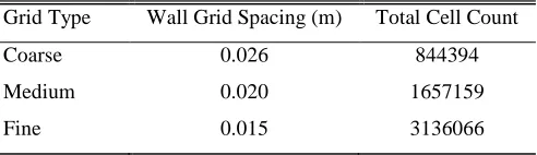
the properties shown in Table. 1. These grids were used to conduct a grid independence study

to select the most appropriate grid density (13,14) with the correct balance between solution

accuracy and efficient computation.

Table. 1: Grid properties.

Grid Type Wall Grid Spacing (m) Total Cell Count

Coarse 0.026 844394

Medium 0.020 1657159

Fine 0.015 3136066

Boundary conditions

Flow boundary conditions must be specified on inlets and outlets, and in some cases it is

necessary to specify conditions such as temperature distributions on walls and other surfaces.

In the simulations presented here, inlet flow boundary conditions were determined through

physical experiments (23) using a balometer (TSI Airflow PH721, 42 to 4250 m3/h ±3%, TSI

Incorporated, Shoreview, Minnesota, USA) to measure total volumetric flow rate and a

low-range anemometer (Testo 435 and comfort level probe, 0 to 5 m/s ±0.03 m/s, Testo Ltd.,

Alton, Hampshire, UK at 66 points to measure the velocity profile). The measured velocity

profiles and air inlet angles were used to define velocity inlet type boundary conditions in the

CFD model together with the turbulence intensity, TI=5%, and the hydraulic diameter,DH = 0.315 m. The outflow conditions are modeled using pressure outlet type boundary conditions

with a local static pressure of -10 Pa. All wall boundaries are assumed adiabatic, as there were

no substantial heat gains in the chamber.

Turbulence models

The characteristics of the computed flow field depend critically on the way in which

Reynolds Averaged Navier-Stokes (RANS) turbulence models which account for common

features of airflow patterns such as recirculation regions and wall-bounded (entrained) flows

(13,14). These features are particularly important in the upper region of the chamber

considered in the present study. Although more advanced methods exist for simulating

turbulence such as Large Eddy Simulation (LES) and Direct Numerical Simulation (DNS), the

vast computational requirements are prohibitive for a parametric study of this nature.

The mixing effect induced by turbulence is known to potentially reduce the effectiveness

of in-duct UV air applications by reducing the effective residence time (24), but this parameter

has not been assessed in detail for upper-room UV scenarios. Further studies have also shown

that the choice of turbulence model for simulating disinfection rates in water applications has a

marked effect on flow structure (17,25), however, to the authors knowledge there are no

equivalent studies for room-scale air disinfection. Thus four commonly-used turbulence

models are considered in the present study, namely:

1. Standardk-ε (SKE) (26)

2. RNG k-ε (RNG) (27)

3. Standardk-ω(SKO) (28)

4. Reynolds Stress Model (RSM) (29,30)

The first three are referred to as two-equation models because they encompass two

transport equations, one for the turbulent kinetic energy,k, and a second one for the dissipation of this energy within the flow,ε(noteω =ε /k). In contrast the RSM employs a total of seven

transport equations including six stress tensors which are solved in addition to those forkand ε. The main difference between the RSM and the two-equation models is that the RSM

accounts for anisotropy in the turbulence field whereas the others assume isotropic turbulence.

What this implies is that only the RSM is capable of simulating elongated turbulent eddies

(vortex stretching) which are physical characteristics and typical of indoor airflow patterns

UV models

UV-field definition:A UV irradiance field is readily defined with a CFD model as a static 3-D

scalar field that is independent of the airflow. However, this definition relies on appropriate

field data for the specific device concerned. Modelling approaches are feasible for some

devices, applying lighting laws (32-37) or radiation models (19). However, creating such

models for upper-room devices is not straightforward due to the louvered design and resulting

complexity of the irradiance field.

Empirical data taken from physical measurements (e.g. radiometry or actinometry (1))

is another feasible approach to creating a field model. Noakeset al(9) applied a low resolution fit to limited measurements leading to cos and cos2 relationships which define the field distribution. Sung and Kato (21) adopted the same approach with a limited number of field

measurements. In both these studies assumptions about the field were made with considerably

less than the 1000+ readings taken in full goniometry studies and neither study considered

room-surface reflectance, although it has been suggested it is likely to have minimal impact on

the results (21). Taking these factors into consideration for the present study, a decision was

taken to directly use radiometry measurements within the CFD model and to explore the

impact of field accuracy on model results.

An experimental rig was designed so that readings could be made in the horizontal plane

passing directly through the centre of the UV fixtures. A radiometer (UV SENS and UV LOG,

sglux, SolGel Technologies GmbH, Berlin, Germany) calibrated within the previous year and

with a reading accuracy of 0.5% was mounted to a measurement arm which pivots about a

point directly above the centre of the UV fixture and can be positioned at any pre-determined

horizontal angle within the UV band (Figure 2). In all cases the radiometer always faces the

centre of the fixture thus ensuring that line-of-sight irradiance measurements are taken. A

series of docking holes along the length of the measurement arm permitted radiometry

Figure 2.Illustration of the radiometry measurement apparatus.

Preliminary data highlighted substantial variability in measured UV output with

differences in peak intensity of up to 40% depending on the brand and age of UV lamps

present. Whilst this aspect is beyond the scope of this study, these observations underline the

potential variability of irradiance fields depending on the type of lamps used. For consistency,

both UV fixtures were fitted with brand new lamps (Philips TUV PL-L, 36W, 12W UVC)

which were used for approximately 10 hours prior to the experiments. Although this time is

relatively short, results for both fixtures are comparable and close monitoring of the output

before and after measurements showed consistent readings in contrast to the aforementioned

variability in output for older bulbs. Before each fixture was analysed it was turned on and left

for two hours until the UV output had stabilised. Three sets of measurements were taken (per

fixture) in the horizontal plane which coincides with the centre of the UV band (subsequently

referred to as the central horizontal plane).

Due to symmetry, readings for the large fixture (Lumlier WM236) were only taken in

one half of the room for the following range of angles:θ= 0º, 10º, 20º, 35º, 50º, 65º and 75º.

Measurements taken beyond θ= 75º yielded no UV output because a shadow was cast by the

side wall of the fixture. For the small fixture (Lumalier WM136) the range of necessary

contains only one lamp which has a ceramic end cap at its base creating a non-uniform UV

output and a field skewed slightly towards one side of the room. Consequently the range of

measurement angles considered for the small fixture is: θ= 0º, ±10º, ±20º, ±35º, ±50º, ±65º

and ±67.5º. Due to constraints on the size of the chamber the measurement arm was limited to

1.9 m for angles between ±50º and ±75º and 3.2 m for angles in the range of 0º to ±35º.

Depending on the specific measurement angle, up to 40 measurements were taken along the

length of the arm. With the first measurement (perθ) taken immediately in front of the fixture

(i.e. touching the grilles) the inter-point spacing increases from 0.02 m to 0.20 m at the far end

of the arm. This clustering of readings in the immediate vicinity of the grilles is necessary to

capture the high gradients in the intensity levels. Altogether each set of in-plane measurements

yielded a total of 239 readings for the large fixture and 392 readings for the small one.

Despite the relatively narrow band height of 0.080 m (dictated by the height of the

grilles), the variation in intensity in the vertical direction in addition to the in-plane readings

has been shown to be equally important (21). A carriage controlled by a finely threaded rod

enabled vertical placement giving a total of 21 uniformly-spaced measurement locations, each

0.005 m apart. This device was deployed throughout the room so that the variation of field

intensity in the vertical direction could also be characterised in locations of interest.

Implementation of the measured fields in the CFD model is described in the results section.

UV Dose modelling

UV dose, D (J/m2), is defined as the product of the field, E (W/m2) and the duration of exposure, t (s). In the context of room airflow passing through a spatially varying field the dose has a cumulative effect along a particular air pathway. As such, dose can be evaluated

through a particle tracking approach using an algorithm to sum the dose along the trajectory or

applied as a passive scalar tracer, through defining the rate of change of dose as a sink term

(20). Either approach can be applied to the room air as a whole (20) to optimise general

coverage or the air from a particular source such as an infectious patient (18) where the source

location is known. The present study applies a passive scalar approach (20) where the dose

distribution, D, depends on the irradiance field (E (x,y,z)) and the velocity vector field, U

 

 UD E (2)

Microorganism Inactivation models

Models simulating microorganism inactivation require several assumptions to be made

including the susceptibility characteristics of the pathogen, the location of the source and, in

the case of particle tracking methods, assumptions about the size and mass of particles. In

many scenarios a source location can be assumed; simulations that compare to experimental

studies generally have a well defined source location (20) while in assessment of hospital ward

type spaces it is often reasonable to assume the location of an infectious patient (18).

Similarly, data on size and mass of particles can be approximated from knowledge of

respiratory droplet sizes. All air disinfection studies to date have simulated microorganism

susceptibility using the first-order decay assumption, applying equation 1 as a removal term in

the numerical model. As such results rely on the selection of an appropriate susceptibility

constant,Z, typically derived from single-pass experiments.

Simulations conducted here use a similar approach to previous scalar tracers studies,

however a gas phase (N2O) species model rather than a passive tracer is applied. This is more

realistic for comparison with ventilation tracer gas studies (36) and overcomes technical

difficulties with implementing the inactivation source terms within the Fluent CFD software.

Microorganism inactivation (equation 1) is coupled to the species transport equation, namely:

 

_

_

_

_

S S Y S

U Y t

Y _{    }



  _{ }

(3)

whereρis the species density (Kg/m3),Yis the species concentration,t is the time (s) ΓSis the species diffusion coefficient and SS represents the species sink term (i.e. removal of microorganism due to interaction with the UV field). In all simulations where inactivation is

considered, the source is located at the geometric centre of the room (Figure 1) and defined by

a constant source value over a volume of 0.00375 m3. In all the results, inactivation is

Simulation set-up

Simulations were conducted using Fluent, version 13.0 (22). In all cases ventilation flows are

assumed constant and simulations conducted as steady state. An isothermal approach was

adopted because the temperature increases due to the presence of the UV lamps were minimal

under the influence of mechanical ventilation and there were no other heat sources present in

the room. Double precision real number representation was employed to minimise round-off

error in the computations and second-order discretisation of all equations (i.e. pressure,

momentum, species and turbulence) ensured they were solved with an acceptable level of

accuracy (13). Solutions were considered to be converged when the residual levels (a measure

of the error in the solutions) showed no signs of changing. Typically this occurred in

2000-15000 iterations depending on the grid density and turbulence model used.

RESULTS

UV field Characteristics

Radiometry measurements in the horizontal plane

Figure 3 shows the measured irradiance field emanating from the large UV fixture as a

function of distance (r)and angle (θ)in a horizontal plane at the centre of the UV band.

The field strength peaks at a value of 4.103 ±0.034 W/m2 along the 10º line of

measurements and approximately 0.4 m from the center of the lamps (0.2 m from the fixture

grilles). Although this peak might be expected to occur along the 0º line (i.e. perpendicular to the

center of the grilles) there is a space between the two lamps in the fixture which explains the slight

dip in intensity compared to the 10º line. As the angle within the measurement plane increases

beyond 10º, the intensity gradually reduces until it dramatically weakens for the two largest

angles. The distinct dip in intensity along the 65º line can be explained by a small shadow cast by

Figure 3.Radiometry measurements taken in the central horizontal plane for the large UV fixture. Error bars determined from the standard deviation of three measurement sets.

As expected, the UV intensity produced by the small UV fixture (Figure 4) is weaker both

in terms of the observed peak intensity (3.728 ±0.033 W/m2) and its projection into the room. The

aforementioned skewing of the field is particularly evident for larger angles (e.g. 67.5° compared

to -67.5°) although this characteristic is less noticeable for smaller angles where the output is

uniform. Again pronounced dips in the intensity are seen near to the device for a number of

measurement lines which is due to the small shadows produced by the grille posts. The error bars

are greatest for measurements close to the grilles which may be due to interference from the grille

plates; significantly reduced error bars are associated with measurements taken further away from

the grilles.

0.0 0.5 1.0 1.5 2.0 2.5 3.0

0.0 0.5 1.0 1.5 2.0 2.5 3.0 3.5 4.0 4.5

0 degrees 10 degrees 20 degrees 35 degrees 50 degrees 65 degrees 75 degrees

E

(W

/m

2 )

Figure 4.Radiometry measurements taken from the central horizontal plane for the small fixture for (a) positive and (b) negative angles. Error bars determined from the standard deviation of three measurement sets.

0.0 0.5 1.0 1.5 2.0 2.5 3.0

0.0 0.5 1.0 1.5 2.0 2.5 3.0 3.5 4.0 4.5

0.0 0.5 1.0 1.5 2.0 2.5 3.0

Radiometry measurements in the vertical direction

Figure 5 shows how the UV field varies with height, h, and the distance away from each device,r, along the 0° measurement line.

Figure 5.Three-dimensional plots showing the extent of UV beam spreading as a function of the horizontal and vertical distance within the UV band for (a) the large device and (b) the smaller

The UV band height increases from 0.05 m near the grilles up to 0.10 m at a distance of 2.15

m from each fixture. For the large fixture, the vertical distribution develops from an initial

square and narrow band to a Gaussian form which reduces in peak intensity with increasing

distance from the grilles. The small fixture exhibits asymmetry in the near-grille profiles

which is attributable to misaligned grilles and minor shadows affecting the intensity; this

illustrates one of the subtleties of real-world UV field characteristics and how the practical

implementation of perfectly parallel grille plates cannot be guaranteed. The observed skewness

in the vertical profile becomes less pronounced further away from the fixture as the influence

from the grilles diminishes. The field produced by both fixtures exhibits beam-spreading

which, in the case of the large fixture, results in a small but measurable region of UV output

beyond the extent of the grilles. Although not presented here, the vertical field distribution was

also assessed for measurement angles of 35° and 50°; the results followed the same trend as

those shown in Figure 8, but with a corresponding reduction in peak intensity observed.

Irradiance field curve fitting and implementation within the CFD model

Implementing experimental irradiance measurements within the CFD model requires

translation of the data into a form which matches the CFD grid. Each cell can only contain a

discrete value for irradiance, therefore interpolation is required to map the experimental

readings onto this grid structure. The programming language Gri, version 2.12.23 (37) was

used as a curve-fitting tool utilising Barnes interpolation (38). The resulting function

represented the field well and was within 0.5% of measured values across the majority of both

fields. Minor differences were apparent in the central horizontal plane with peak values

underestimated by 6.1% and 12.4% for the large and smaller fixtures respectively. This was

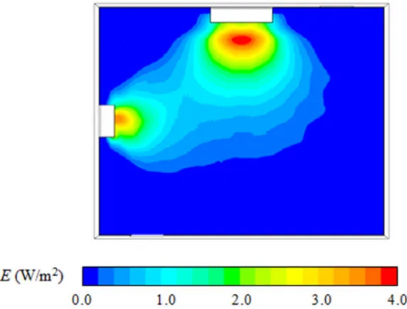
considered acceptable as peak values only occur in a small region of the room. Figure 6 shows

the irradiance field implemented in the CFD software, in the central horizontal plane with both

devices active using the curve-fitting methodology described above.

Field distribution in the vertical direction was interpolated from the data using two

approaches; a 3D field approximated by 5 sub-bands corresponding to the CFD grid (Figure

7(a)) and a 2D field with constant intensity in the vertical direction (Figure 7(b)). A third, 1D

for comparison. Whilst the peak intensity increases with the number dimensions, all three

fields gave the same overall output. The volume-averaged field intensity throughout the UV

region (band comprising height of fixture) is 0.05467 W/m2 for the smaller fixture and

0.15972 W/m2for the larger one.

Figure 6.Contour plot of the irradiance field produced by both fixtures in the aerobiology chamber.

Figure 7.Contour plots of a section of the vertical plane intersecting the center of the large

Model Parameter Sensitivities

Grid and turbulence sensitivity

Simulations with the high-in ventilation regime at 6ACH and the 2D UV field were run on

three grids (Table 1) in conjunction with the four turbulence models; the standard k-ε model

(SKE), RNG k-ε (RNG), Standard k-ω (SKO), and the Reynolds Stress Model (RSM). For

each of these grid-turbulence model combinations, three parameters were evaluated, the

volume-averaged dose within the room, Dave (J/m2), the volume-averaged velocity magnitude in the UV zone,Umag(m/s), and a dimensionless mixing factor,β, which is given by:

inlet uv

Q U A

 

2 int

 (4)

where: Auv(m2) is the area of the interface separating the UV zone and the main room volume immediately below it,Uint(m/s) is the mean absolute vertical velocity at the interface andQinlet (m3/s ) is the room supply flow rate (10).

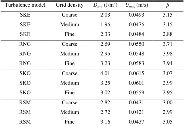
Table. 2: Influence of grid and turbulence model on dose and flow parameters

Turbulence model Grid density Dave(J/m2) Umag(m/s) β

SKE Coarse 2.03 0.0493 3.15

SKE Medium 1.96 0.0476 3.15

SKE Fine 2.33 0.0484 2.88

RNG Coarse 2.69 0.0550 3.71

RNG Medium 2.95 0.0548 3.98

RNG Fine 3.23 0.0583 3.94

SKO Coarse 4.01 0.0615 3.07

SKO Medium 3.25 0.0601 2.99

SKO Fine 3.02 0.0559 2.95

RSM Coarse 2.82 0.0431 3.00

RSM Medium 2.72 0.0421 2.99

RSM Fine 3.16 0.0437 3.05

Table 2 shows variation with grid density for all turbulence models tested, however the

parameters are of a similar magnitude across all the simulations. The errors between the

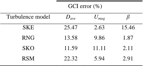
Table 3 summarises the GCI errors for the three parameters showing variability in

performance of the turbulence models both in terms of the UV-related quantity (Dave) and airflow parameters (Umagandβ). Taking the results from Tables 2 and 3 into consideration, the logical choice of grid to be used in all subsequent simulations is the fine one which contains

3.14 million cells i.e. ~0.1 million cells/m3.

Table. 3: Discretization errors determined from the Grid Convergence Index (39) for various

solution parameters.

GCI error (%)

Turbulence model Dave Umag β

SKE 25.47 2.63 15.46

RNG 13.58 9.86 1.87

SKO 11.59 11.11 2.11

RSM 22.32 5.94 2.91

The influence of turbulence model on airflow structure and hence dose is shown in

Figures 8 and 9. Contour plots of dose (Figure 8) show similar results for the SKE and RSM

models (Figures 8(a) and (d)), while the RNG model (Figure 8(b)) predicts a more pronounced

region of high dose in front of the large UV fixture (D > 30 J/m2). This model predicts the highest room-average dose and mixing factor suggesting the turbulence model leads to a

higher predicted level of mixing. The SKO model exhibits a dose contour plot which is the

Figure 8.Contour plots of the dose,D, in the central horizontal plane for (a) SKE, (b) RNG, (c) SKO and (d) RSM turbulence models. The ventilation rate is 6ACH, both UV fixtures are

active and the flow regime is in-high, out-low.

Figure 9 compares airflow pathlines (not particle tracks) originating at the centre of the

room. With the exception of the SKO case, all of the flow patterns are initially directed

towards the inlet before mixing throughout the room. The pathlines produced by both of the

k-ε models (SKE and RNG) exhibit the most uniform spreading in the space (Figures 9(a) and

(b)), however these diffusion-dominated flow fields are strongly influenced by the diffusive

nature ofk-ε-type turbulence models. The observed pathlines for the RSM model (Figure 9(d))

clearly show a mixture of large and small-scale turbulent structures in addition to elongated

eddies (vortex stretching) near to the inlet. These flow patterns can be expected for this

turbulence (14,31). The pathlines produced by the SKO model reveals the most unusual flow

pattern of all the turbulence models tested with noticeably less flow dispersal present. This can

be explained by the fact that the simulations of the airflow using this particular model

exhibited numerical noise, even after convergence had been attained and this undoubtedly

affected the result.

Figure 9.Pathlines released from the center of the room and colored by the dose,D, for (a)

SKE, (b) RNG, (c) SKO and (d) RSM turbulence models. The ventilation rate is 6ACH, both UV fixtures are active and the flow regime is in-high, out-low.

All subsequent simulations are conducted using the RSM model as it has an acceptable

degree of accuracy, the most physically-correct flow structure and has recently been shown to

UV Field Sensitivity

Simulations of the high-in flow regime for a ventilation rate of 6ACH were conducted for

three UV fixture combinations: (i) both active, (ii) large fixture only and (iii) small fixture

only. Figure 10 presents the influence of the field models on room average dose (Dave)

received by the incoming air for all three fixture combinations and predicted inactivation for

an airborne microorganism released at the centre of the room for case with both fixtures active

only. In the latter case, simulations were conducted for microorganism susceptibilities ranging

from z = 0.01 to z = 1.50 (m2/J). As the field resolution reduces simulations increasingly

over-estimate dose for all three lamp configurations (Figure 10(a)). The 2D field is a good

approximation, only over-predicting dose by 11-12%. However the 1D field is clearly a poor

representation, over-estimating dose by 37-53%. This behavior is also apparent in the resulting

prediction of microorganism inactivation (Figure 10(b)); the 1D field again over-predicts,

while the difference between the 2D and 3D fields is almost indistinguishable. In order to

highlight the variability of dose, error bars are determined from the standard deviation of Dave measured at 529 evenly distributed points throughout the room (Figure 10(a)). Although the

mean values of Davevary significantly depending on the type of UV field used, the variability is proportionately very similar in each case.

Figure 10. Influence of field model on (a) room averaged dose,Davefor three lamp

combinations and (b) predicted inactivation for both fixtures operating together, as a function of microorganism susceptibility,z

Both devices Large device Small device 0 1 2 3 4 5 6

Z(m2/J)

Da

ve

(J

/m

2 )

3D field 2D field 1D field

0.0 0.3 0.6 0.9 1.2 1.5

0 20 40 60 80 I (% )

3D field 2D field 1D field

Impact of Surface Reflections

Surface reflection is known to be important for “in-duct” UVGI systems and studies have dealt

with reflections by assuming that irradiance levels measured on surfaces essentially become

sources which reflect the UV energy back into the space of interest (40). Such methods are

very difficult to implement in conjunction with experimentally measured values (as used in

this study) and may be an unnecessary complication. To evaluate the significance of

reflections for upper-room application, the central horizontal plane measurements for both UV

fixtures were analyzed to determine field intensity along imaginary boundaries. These

represented extremities of different sized rooms from (1.0 m x 1.0 m) to (3.0 m x 3.0 m). Table

4 compares the average perimeter irradiance, Eper (W/m2) to the plane-average irradiance,

Eave,using the relative irradiance,RE:

ave per E

E E

R  (5)

Table. 4: The effect of perimeter size on absolute and relative irradiance measurements.

Eper(W/m2) RE

Room plan area (m2) Large fixture Small fixture Large fixture Small fixture

1.0 1.225 0.393 0.785 0.478

1.5 0.487 0.100 0.469 0.211

2.0 0.205 0.009 0.299 0.034

2.5 0.068 0.004 0.143 0.025

3.0 0.019 0.002 0.058 0.019

The irradiance measured along the 1.0 m perimeter for both fixtures is similar in

magnitude to the to the average value, however, this can be considered an unrealistically-small

room as can the 1.5 m and 2.0 m perimeters; these cases are merely shown for illustrative

purposes. As the perimeter increases to 3.0 m which is representative of a small room (e.g.

single-bed hospital ward), the realtive intensity drops to 5.8% and 1.9% for the large and small

fixtures respectively. In absolute terms, the perimeter-average irradiance of 0.019 W/m2for the

region (0.002 W/m2(1)). This is a small reading considering the fact that the measurements are

taken in the centre of the UV band where the output is greatest. An implication of this result is

that surface reflections produced by the upper-room UV fixtures considered in this study are

only significant in very small rooms; in larger spaces the substantial drop in intensity far away

from the fixture leads to practically insignificant reflections.

UV-Airflow Interaction

A parametric study was carried out using the 2D field model with RSM turbulence and no

reflections to explore the influence of ventilation rate, ventilation regime and device operation

on both predicted dose and inactivation. Results consider both room averaged effects and

spatial distributions.

Predicted Dose

Figure 11 shows how room averaged dose reduces with ventilation rate due to the lower

residence time of the air in the room. However both the magnitude and the extent of reduction

depend on the UV fixtures and the ventilation regime. A markedly higher dose is predicted

with the low level ventilation supply, with values up to a third higher for the same fixture

configuration. This result is consistent with earlier studies which show that upper room UVGI

is most effective in rooms with ventilation rates of 6 ACH or lower (6).

Figure 11. influence of room ventilation rate and regime on the room average dose received by

the air entering the room.

0 3 6 9 12 15

0 3 6 9 12

Da

v

e

(J

/m

2 )

In-low: both fixtures In-low: large fixture In-low: small fixture In-high: both fixtures In-high: large fixture In-high: small fixture

Figure 12 considers the variation in dose by zone at 6 ACH, with volume averaged

dose also calculated for the upper-zone of the room (region containing the devices and above)

and lower-zone (below the devices, “occupied” zone) as well as the room average value.

Results show the increase in dose is seen across both zones, and also indicates that for all

fixtures and both flow regimes, the room averaged dose is a good indication of the average in

the occupied (lower) zone. Figures 13 and 14 consider variability in the dose on a horizontal

plane at a height of 1.5 m (equivalent to an occupant breathing zone). It can be seen that in

both cases, while the small device results in a lower dose, the spatial distribution is more

clustered and the average dose on the plane is representative. The large device and both

devices operating together result in more variance across the plane, particularly with the

low-high ventilation regime. For example, Figure 13(c) shows that while the plane average dose is

3.34 J/m2, the dose varies from below 1 J/m2 to almost 10 J/m2, indicating areas of low and

high coverage.

Figure 12. Average dose calculated for whole room, upper region of the room only and lower

region of the room only (a) low-high and (b) high-low ventilation regime

Results in Figures 11-13 should be treated with some caution; they are specific to the

particular room and should not be interpreted as one ventilation approach is better than

another. However, they do indicate that airflow pattern can have a significant impact on device

effectiveness, both in terms of overall effect and spatial coverage.

Both devices Large device Small device

0 1 2 3 4 5 6 7 (a) (b) D (J /m 2 ) Room average Upper zone Lower zone

Both devices Large device Small device

Figure 13. Dose histograms at 6ACH with ventilation regime low-high (a) both fixtures, (c) large and (e) small; high-low regime (b) both fixtures, (b) large and (f) small. (5305 samples taken from

breathing plane i.e. y = 1.5 m)

Inactivation

Figure 14 considers predicted microorganism inactivation with ventilation parameters, UV

fixture and microorganism susceptibility. Room average inactivation follows dose

predictions; inactivation is higher with increase in the UV field intensity and with a low-high

ventilation regime for this particular room (Figure 14(a)). As ventilation rate increases,

relative inactivation drops due to the greater influence of dilution (Figure 14(b)). As with

dose, consideration of the spatial distribution is also important for real applications. Figure 15

0 2 4 6 8 10

0 10 20 30 40 (e) (f) (c) (d) F re q u en cy (% ) F re q u en cy (% )

D_mean=3.34 J/m2 D_mean=2.29 J/m2

D(J/m2)

D(J/m2

)

D_mean=4.80 J/m2 D_mean=3.18 J/m2

F re q u en cy (% )

D(J/m2) D(J/m2)

D(J/m2)

D(J/m2)

F re q u en cy (% ) F re q u en cy (% ) F re q u en cy (% ) F re q u en cy (% ) F re q u en cy (% )

0 2 4 6 8 10

0 10 20 30 40 (a) (b)

0 2 4 6 8 10

0 10 20 30 40 F re q u en cy (% )

0 2 4 6 8 10

0 10 20 30 40

0 2 4 6 8 10

0 10 20 30 40

D_mean=1.47 J/m2

D_mean=0.90 J/m2

0 2 4 6 8 10

indicates how the local flow rate influences the relative microorganism concentration across

the room and that in neither case the UV is able to influence the concentration close to the

source.

Figure 14. Influence of ventilation and UV device parameters on predicted inactivation (a)

influence of microorganism susceptibility, (b) influence of ventilation rate.

Figure 15. Contour plots showing predicted microorganism distribution in the breathing

plane (y = 1.5 m) with ventilation rate of 6 ACH and both fixtures active for (a) low-high and (d) high-low flow regimes.

0.0 0.3 0.6 0.9 1.2 1.5

0 20 40 60 80 100

I

(%

)

In-low: both fixtures In-high: both fixtures In-low: large fixture In-high: large fixture In-low: small fixture In-high: small fixture

Z(m2/J)

0 3 6 9 12 15

0 20 40 60 80 100

(a) (b)

Z= 0.2 (m2_/J)

Ventilation rate (ACH)

I

(%

)

In-low: both fixtures In-high: both fixtures In-low: large fixture In-high: large fixture In-low: small fixture In-high: small fixture

DISCUSSION

Simulation Accuracy

The CFD results presented in the investigation highlighted the sensitivity of the grid density,

turbulence model selection, UV field and considered surface reflectance. Results show a fine

grid yields more consistent and accurate results both in terms of airflow and UV-specific

parameters and that the RSM turbulence model produces the most physically correct flow

field. However, provided a reasonable degree of care is exercised in developing the geometry,

the grid and turbulence parameters have a relatively small influence on the results. The UV

field definition on the other hand is a much more significant factor in ensuring good results

from simulations. A uniform field assumption is insufficient to give accurate results, leading

to an over-prediction of both dose and inactivation. Results were also compared to previous

studies implementing an empirical 3-D field derived from limited measurements (9,20). While

this approach gives better insight into the spatial variability, the model also over-predicted

dose and inactivation as the vertical UV distribution is assumed uniform based on the peak

horizontal plane data. The 2D and 3D fields used in this study indicate that a 2D field is

sufficient for making predictions. However it should be noted that in creating this field the

uniform intensity across the vertical band was only 57% of the central horizontal plane

measurements, thus ensuring that the overall output of the two fields was the same rather than

over-predicting the total output using the peak values. Had similar factors been used in

Noakes et al (9) it is likely that predictions would have been much closer. Field sensitivity results also suggest that full goniometry is not necessary for modelling purposes. As the 2D

and 3D fields give such close predictions, it suggests that a smaller data set is adequate to

represent the field and that for louvered devices with collimated beams only central plane

readings are required providing a suitable reduction factor is used to translate the readings to a

2-D field.

While the results for the uniform (1D) field are an over prediction, this finding does

highlight the fact that implementing as uniform a field as possible actually leads to greater

effectiveness and concurs with the current NIOSH recommendation for the application of

None of the simulations presented here incorporated surface reflections, as an

evaluation of the relative irradiance indicated the effects are minimal for most practical sized

rooms. Including reflections is not straightforward as it requires further models treating the

incident radiation on walls as a new source. In terms of disinfection potential, the

computational effort outweighs the minimal influence on the field, and results without

reflection will always err on the conservative side. However it should be noted that reflections

may not be insignificant in terms of occupant UV exposure in the lower zone.

Validity and Uncertainty

CFD simulations can be used to predict two key attributes of interest, dose and inactivation.

Providing the airflow and UV field can be modeled with sufficient accuracy (and it is feasible

to validate both without significant challenge) then predictions of dose can be considered

reliable; dose is calculated from a straightforward interaction between the two parameters.

However there is a question as to what does the dose mean? The results in Figures 11-13

highlight that dose depends on fixtures, ventilation rates and ventilation regimes and simply

calculating an average dose does not give insight into the variability of dose within the room.

Dose is a cumulative effect following flow paths and therefore depends on the origin of the

air. In a single pass system (i.e. in-duct UV) the origin is clear; air entering the duct has a zero

dose and dose accumulates as it passes over UV lamps. In a room scenario this is not so clear.

Results presented here consider the dose received by the air entering the room; at the supply

air grille the initial dose is zero and dose accumulates as the air passes through the room and

interacts with the UV field. This is a feasible method where the location of an infectious

source is unknown and the aim is to maximize coverage (20). However if an infectious source

is located in the lower part of the room, their exhaled air will also have a zero dose, as it will

not have yet interacted with the UV field.

Predictions of inactivation are less certain as assumptions must be made regarding the

microorganism. The first uncertainty lies in the location of the infectious source. Unlike dose,

where the room air as a whole can be considered, inactivation models require specifying the

microorganism; while the assumption that the pathogens are truly airborne and behave like a

passive tracer or gas phase is the most straightforward approach, real bioaerosols have mass

and momentum which will influence their behavior. Finally, all simulation studies to date,

including this one, have simulated microorganism susceptibility as exhibiting first-order

decay, applying equation 1 as a removal term in the numerical model. As such, models rely on

the selection of an appropriate susceptibility constant typically derived from single-pass

experiments. There is an assumption that this applies under room scale conditions, however

the incomplete inactivation and multiple airborne microorganism passes between UV and

non-UV zones in an upper-room system mean that repair mechanisms may need to be

considered. Beggset al(12) conducted an experimental study in an incompletely mixed room and suggested effective microorganism susceptibility to upper-room UV may be up to an

order of magnitude less than in single-pass testing, most probably due to the reactivation.

However Xu et al(6) also conducted experiments in a fully mixed room and showed only a small reduction in the calculated susceptibility constant in a room scale scenario. Although

these two findings are in broad agreement, and support the need for good air mixing, further

validation data is required before inactivation models can be used with confidence in

predictive studies.

Current and Future Application of CFD

Role in research and guidance

CFD simulation clearly has a substantial role to play in current and future upper-room UV

research studies. By coupling CFD models with experimental data it already offers an insight

into the disinfection mechanisms, and with sufficient future data will enable validation of the

inactivation models and hence prediction. Chamber based research studies have well-defined

and generally steady state airflows, which can be modelled with confidence using CFD,

allowing the study to focus on UV parameters. While field based studies will have more

transient and complex airflows (see below), CFD simulation could be used to both aid design

of such studies and interpret the results. CFD simulation also has clear potential to assist with

defining appropriate guidance. NIOSH currently recommend a plane-average UV irradiance

However, as shown here, the same device can yield quite different dose and inactivation

results depending on room and ventilation parameters. In addition, such guidance cannot be

easily applied for UV devices that have a diverging beam designed for high ceiling spaces. It

is likely that with suitable field data, CFD simulation can be used to determine appropriate

guidance for other types of fixtures.

Real World Application

Application of CFD simulation to real environments is a greater challenge. While

airflows in isothermal, mechanically ventilated rooms are generally easy to define, the

movement of people and heat gains in real spaces reduces the certainty of the model

predictions. Naturally ventilated spaces are more challenging still as the ventilation flow

patterns will change with weather conditions (41,42). In this situation a single steady-state

model is not likely to be reliable and it will be necessary to conduct transient simulations or,

as a minimum, simulations for a range of cases in order to understand the sensitivity of the

flow and interaction with UV field.

As suggested by previous researchers (21) infection control in healthcare settings

which utilise UVGI systems is not straightforward and needs guidelines to be developed for

effective use and installation. In terms of ventilation, higher flow rates and hence smaller

residence times are required to ensure the efficient removal of microorganisms. However, for

UVGI to be effective, a larger residence time is required to deliver a sufficient dose to induce

a satisfactory level of microorganism inactivation. Striking the correct balance between

infection control measures is one of the most challenging aspects of hospital ward design and

this is likely to be the case for the foreseeable future. Despite this, CFD modelling already

offers a means of better understanding airflow patterns in rooms and insight into (a) the best

location for upper-room UV devices (through simulating dose) and (b) whether the room

would benefit from additional mixing. One of the major strengths of CFD modelling is that

the room-wide dose distribution can be predicted, whereas this simply cannot be done

experimentally. Although predicting the effectiveness of UV systems in terms of

useful insight into the range of performance that could be expected under different

susceptibility assumptions.

ACKNOWLEDGMENTS

study.

REFERENCES

1. NIOSH (2009), Environmental Control for Tuberculosis: Basic Upper-Room Ultraviolet Germicidal Irradiation Guidelines for Healthcare Settings. Centers for Disease Control and Prevention, National Institute for Occupational Safety and

Health.

2. Noakes, C.J., L.A. Fletcher, C.B. Beggs, P.A. Sleigh, and K.G. Kerr. (2004a)

Development of a numerical Model to Simulate the Biological Inactivation of

Airborne Microorganisms in the Presence of Ultraviolet Light. Journal of Aerosol Science.35, 489-507.

3. Peccia, J, H.M. Werth, S.L. Miller and M.T. Hernandez. (2001) Effects of relative

humidity on the ultraviolet induced inactivation of airborne bacteria.Aerosol Science and Technology.35, 728-740.

4. Peccia, J and M.T. Hernandez. (2001) Photoreactivation in airborne Mycobacterium

parafortuitum.Applied Environmental Microbiology.67, 4225-4232.

5. Miller, S.L. M.T. Hernandez, K.P. Fennelly, J.W. Martyny, J. Macher, E. Kujundzic,

et al. (2002) Efficacy of ultraviolet irradiation in controlling the spread of tuberculosis. NIOSH final report, Contract 200–97–2602; NTIS publication PB2003-103816. Cincinnati, OH: US Department of Health and Human Services, Centers for

Disease Control and Prevention.

6. Xu, P. J., J. Peccia, P. Fabian, J.W. Martyny, K.P. Fennelly, M. Hernandez and S.L.

Miller. (2003) Efficacy of ultraviolet germicidal irradiation of upper-room air in

inactivating airborne bacterial spores and mycobacteria in full-scale studies.

7. Riley, R.L. and S. Permutt. (1971) Room air disinfection by ultraviolet irradiation of

upper air.Archives of Environmental Health.22, 208-219.

8. Nicas, M. and S.L. Miller. (1999) A multi-zone model evaluation of the efficacy of

upper-room air ultraviolet germicidal irradiation. Applied Occupational and Environmental Hygiene.14, 317 – 328.

9. Noakes, C.J., C.B. Beggs and P.A. Sleigh. (2004c) Modelling the Performance of

Upper Room Ultraviolet Germicidal Irradiation Devices in Ventilated Rooms:

Comparison of Analytical and CFD Methods.Indoor Built Environment.13, 477-488. 10. Beggs, C.B. and P.A. Sleigh. (2002) A quantitative method for evaluating the

germicidal effect of upper room UV fields. Journal of Aerosol Science. 33, 1681-1699.

11. Noakes, C.J., C.B. Beggs and P.A. Sleigh. (2004) Effect of Room Mixing and Ventilation Strategy on the Performance of Upper Room Ultraviolet Germicidal Irradiation Systems. ASHRAE IAQ Conference, Tampa, Florida, 15-17th March. 12. Beggs, C.B., C.J. Noakes, P.A. Sleigh, L.A. Fletcher and K.G. Kerr. (2006)

Methodology for determining the susceptibility of airborne microorganisms to

irradiation by an upper-room UVGI system.Journal of Aerosol Science.37, 885-902. 13. Sorensen, D.N. and P.V. Nielsen. (2003) Quality Control of Computational Fluid

Dynamics in Indoor Environments.Indoor Air.13, 2-17.

14. Li, Y. and P.V. Nielsen. (2011) CFD and ventilation research. Indoor Air. 21(6), 422-453.

15. Memarzadeh, F, Z. Jiang, and W. Xu. (2004)Analysis of efficacy of UVGI inactivation of airborne organisms using Eulerian and Lagrangian approaches. ASHRAE IAQ Conference, Tampa, Florida, 15-17th March.

16. Alani A, I.E. Barton, M.J. Seymour, L.C. Wrobel. (2011) Application of Lagrangian

particle transport model to tuberculosis TB bacteria UV dosing in a ventilated

isolation room.International Journal of Environmental Health Research.11, 219-228. 17. Wols, B.A., W.S.J. Uittewaal, J.A.M.H. Hofman, L.C. Rietveld and J.C. van Dijk.

(2010) The Weaknesses of a k-ε model compared to a large-eddy simulation for the

18. Sung, M. and S. Kato. (2011) Estimating the germicidal effect of upper-room UVGI

system on exhaled air of patients based on ventilation efficiency. Building and Environment.46,2326-2332.

19. Li, C., C.B. Deng and C.N. Kim. (2010) Simulations to Determine the Disinfection

Efficiency of Supplementary UV Light Devices in a Ventilated Hospital Isolation

Room.Indoor Built Environment.19(1), 48-56.

20. Noakes, C.J., P.A. Sleigh, L.A. Fletcher and C.B. Beggs. (2006) Use of CFD

Modelling to Optimise the Design of Upper-Room UVGI Disinfection Systems for

Ventilated Rooms.Indoor and Built Environment.15(4), 347-356.

21. Sung, M. and S. Kato. (2010) Method to Evaluate UV Dose of Upper-Room UVGI

System Using the Concept of Ventilation Efficiency. Building and Environment. 45,

1626-1631.

22. ANSYS (2012) Ansys Inc. http://ansys.com/products/fluid-dynamics

23. King, M.F., M.A. Camargo-Valero, C.J. Noakes and P.A. Sleigh. (2011) CFD validation of controlled bioaerosol release for simulating droplet transmission of live pathogens. Indoor Air 2011, Austin, Texas, 4-10thJune.

24. Chang, D. and C. Young. (2007). Effect of Turbulence on Ultraviolet Germicidal

25. Liu, D., C. Wu, K. Linden and J. Ducoste. (2007) Numerical simulation of UV

disinfection reactors: Evaluation of alternative turbulence models. Applied Mathematical Modelling.31, 1753-1769.

26. Launder, B.E. and D.B. Spalding. (1974) The Numerical Computation of Turbulent

Flows.Computer Methods in Applied Mechanics and Engineering.3, 269-289.

27. Yakhot, V., S.A. Orszag, S. Thangam, T.B. Gatski and C.G. Speziale. (1992)

Development of Turbulence Models for Shear Flows by a Double Expansion

Technique.Physics of Fluids A.4(7), 1510-1520.

28. Wilcox, D.C, 1998, Turbulence modelling for CFD,La Canada, CA: DCW Industries Inc, 173-174.

29. Launder, B.E., G.J. Reece and W. Rodi. (1975) Progress in the Development of a

Reynolds-Stress Turbulence Closure.Journal of Fluid Mechanics.68(3), 537-566. 30. Launder, B.E. (1989) Second-Moment Closure: Present... and Future?, International

Journal of Heat and Fluid Flow.10(4), 282-300.

31. Schalin, A. and P.V. Neilsen. (2004) Impact of Turbulence Anisotropy Near Walls in

Room Air Flow.Indoor Air,14, 159-168.

32. Dumyahn, T. and M. First. (1999) Characterization of ultraviolet upper room air

disinfection devices. American Industrial Hygiene Association Journal. J. 60, 219-227.

33. Rudnick, S.N. (2001) Predicting the ultraviolet radiation distribution in a room with

multilouvered germicidal fixtures. American Industrial Hygiene Association Journal.

62, 434-445.

34. Kowalski, W.J., W.P. Bahnfleth, D.L. Withham, B.F. Severin, and T.S. Whittam.

(2000) Mathematical Modeling of UVGI for Air Disinfection. Quantitative Microbiology.2, 249-270.

35. Kowalski, W.J., W.P. Bahnfleth and R.G. Mistrick. (2005) A Specular Model for

UVGI Air Disinfection Systems.IUVA News.7(1), 19-26.

36. Noakes C.J., L.A. Fletcher, P.A. Sleigh, W.B. Booth, B. Beato-Arribas and N.

37. Gri (2012) gri.sourceforge.net/index.php

38. Barnes, S.L. (1964) A Technique for Maximizing Details in Numerical Weather Map

Analysis.Journal of Applied Meteorology.3, 396-409.

39. Roache, P.J. (1994) Perspective: A Method for Uniform Reporting of Grid Refinement

Studies,Journal of Fluids Engineering.116, 405-413.

40. Kowalski, W.J. (2009) Ultraviolet Germicidal Irradiation Handbook: UVGI for Air and Surface Disinfection. Springer-Verlag, Berlin, Heidelberg. ISBN: 978-3-642-01998-2.

41. Escombe, A.R., C.C. Oeser, R.H. Gilman, M. Navincopa, E. Ticona, W. Pan, C.

Martinez, J. Chacaltana, R. Rodrigues, D.A.J. Moore, J.S. Friedland and C.A. Evans.

(2007). Natural ventilation for the prevention of airborne contagion, Plos Medicine.

4(2), 309-317.

42. Camargo-Valero, M.A., C.A. Gilkeson, C.J. Noakes and P.A.Sleigh. (2010). An Experimental Study of Natural Ventilation Characteristics and Pathogen Transport in Open and Partitioned Hospital Wards. Proceedings of the 9th UK Conference on Wind Engineering, Bristol, UK, 75-78. ISBN: 978-1-4461-8958-0.

FIGURE CAPTIONS

Figure 1.Illustration of the aerobiology chamber with in-high, out-low ventilation regime

depicted.

Figure 2.Illustration of the radiometry measurement apparatus.

Figure 3.Radiometry measurements taken in the central horizontal plane for the large UV

fixture. Error bars determined from the standard deviation of three measurement sets.

Figure 4.Radiometry measurements taken from the central horizontal plane for the small fixture

for (a) positive and (b) negative angles. Error bars determined from the standard deviation of three

measurement sets.

horizontal and vertical distance within the UV band for (a) the large device and (b) the smaller

one. Measurements taken at the intersection of grid lines.

Figure 6.Contour plot of the irradiance field produced by both fixtures in the aerobiology

chamber.

Figure 7.Contour plots of a section of the vertical plane intersecting the center of the large

fixture illustrating (a) 3D, (b) 2D and (c) 1D fields respectively.

Figure 8.Contour plots of the dose,D, in the central horizontal plane for (a) SKE, (b) RNG, (c) SKO and (d) RSM turbulence models. The ventilation rate is 6ACH, both UV fixtures are

active and the flow regime is in-high, out-low.

Figure 9.Airflow pathlines released from the center of the room and colored by the dose,D, for (a) SKE, (b) RNG, (c) SKO and (d) RSM turbulence models. The ventilation rate is 6ACH,

both UV fixtures are active and the flow regime is in-high, out-low.

Figure 10. Influence of field model on (a) room averaged dose,Davefor three lamp

combinations and (b) predicted inactivation for both fixtures operating together, as a function

of microorganism susceptibility,z. Note that the error bars in (a) are determined from the standard deviation ofDavemeasured at 529 points which are evenly spread throughout the room.

Figure 11. influence of room ventilation rate and regime on the room average dose received by

the air entering the room.

Figure 12. Average dose calculated for whole room, upper region of the room only and lower

region of the room only (a) low-high and (b) high-low ventilation regime. Error bars determined

from the standard deviation ofDavetaken from evenly distributed points throughout the applicable portion of the room.

Figure 13. Dose histograms at 6ACH with ventilation regime low-high (a) both fixtures, (c)

large and (e) small; high-low regime (b) both fixtures, (b) large and (f) small. (5305 samples taken

throughout the entirety of the breathing plane i.e. y = 1.5 m).

Figure 14. Influence of ventilation and UV device parameters on predicted inactivation (a)

Figure 15. Contour plots showing predicted microorganism distribution in the breathing

plane (y = 1.5 m) with ventilation rate of 6 ACH and both fixtures active for (a) low-high and