Distributed LQR Design for a Class of Large-Scale Multi-Area Power Systems

City, University of London Institutional Repository

Citation

: Vlahakis, E. E., Dritsas, L. and Halikias, G. ORCID: 0000-0003-1260-1383

(2019). Distributed LQR Design for a Class of Large-Scale Multi-Area Power Systems.

Energies, 12(14), 2664.. doi: 10.3390/en12142664

This is the published version of the paper.

This version of the publication may differ from the final published

version.

Permanent repository link:

http://openaccess.city.ac.uk/id/eprint/22748/

Link to published version

: http://dx.doi.org/10.3390/en12142664

Copyright and reuse:

City Research Online aims to make research

outputs of City, University of London available to a wider audience.

Copyright and Moral Rights remain with the author(s) and/or copyright

holders. URLs from City Research Online may be freely distributed and

linked to.

Article

Distributed LQR Design for a Class of Large-Scale

Multi-Area Power Systems

Eleftherios Vlahakis1,* , Leonidas Dritsas2 and George Halikias1

1 _{Department of Electrical & Electronic Engineering, City, University of London, London EC1V 0HB, UK} 2 _{Department of Electrical & Electronic Engineering Educators, School of Pedagogical & Technological}

Education, ASPETE, 14121 Athens, Greece * Correspondence: [email protected]

Received: 16 June 2019; Accepted: 9 July 2019; Published: 11 July 2019

Abstract: Load frequency control (LFC) is one of the most challenging problems in multi-area power systems. In this paper, we consider power system formed of distinct control areas with identical dynamics which are interconnected via weak tie-lines. We then formulate a disturbance rejection problem of power-load step variations for the interconnected network system. We follow a top-down method to approximate a centralized linear quadratic regulator (LQR) optimal controller by a distributed scheme. Overall network stability is guaranteed via a stability test applied to a convex combination of Hurwitz matrices, the validity of which leads to stable network operation for a class of network topologies. The efficiency of the proposed distributed load frequency controller is illustrated via simulation studies involving a six-area power system and three interconnection schemes. In the study, apart from the nominal parameters, significant parametric variations have been considered in each area. The obtained results suggest that the proposed approach can be extended to the non-identical case.

Keywords:multi-area power system; large-scale power system; distributed load frequency control; automatic generation control; interconnected control areas; secondary frequency control; distributed linear quadratic regulator; distributed optimal control

1. Introduction

Power systems are important in engineering, and their stable and continuous operation is inherently connected to social welfare and economic prosperity. Power system networks can be characterized as large-scale complex systems which encompass a broad array of subsystems and tasks. This intrinsic complexity is constantly evolving and growing in alignment with state-of-the-art technologies, facilitating a more efficient power generation, transmission, and distribution. Recently, the increasing penetration of sustainable energy sources into the energy map and the digitalization of power control systems have resulted in sophisticated concepts, such as intelligent power networks and smart grids. The stochasticity and intermittency of renewable energy sources, along with the decentralization of power generation and the integration of unsafe communication layers across the physical structure of the power network, are just a few of the vital reasons that render the control of the modern power systems highly challenging.

In this paper, we consider power system networks formed of distinct control areas which are interconnected via weak transmission lines referred to as tie-lines. Each area maintains a single nominal frequency across its geographical region and is comprised of either a single or a group of generators. In order for an area to maintain its frequency under load variations in the case of multiple generators, a local load frequency controller is used, distributed to the corresponding turbine-governing systems of each generating unit. The design of load frequency control (LFC) is based on a single-plant model

which represents the sum of the generating units [1]. The area is responsible for meeting power demand of its own consumers, as well as of certain adjacent areas with which power exchange is normally scheduled for a contracted value. However, due to power load differentiation, the frequency of each area, along with the scheduled power exchange with its interconnected peers, may vary from their nominal value.

The rate of change of frequency (RoCoF) is related to the power system inertia and the active power mismatch. The relationship between inertia of a distinct area, RoCoF, and change in active power can be found in [2,3]. Virtually, synchronous machines have been the main source of system inertia, hence the area frequency is directly coupled to the rotational speed of the aggregated synchronous generators [2,4]. Traditionally, the prime mover of conventional thermal power stations and hydroelectric plants, along with the synchronous generators (typically of large inertia), act as smoothing (low-pass) filters on variations of electric loads and participate primarily in the frequency regulation of the area. In contrast, renewable energy generation units behave differently from conventional synchronous generators, mostly because they are connected through power electronic interfaces. In effect, these devices fully or partly can electrically decouple the generator from the grid [3], hence the coupling between the rotational speed of the generator and the system frequency is eliminated [5]. For this reason, unlike synchronous generators, inverter-connected generation units do not inherently contribute to the total system inertia [6]. Although control strategies for participation in frequency regulation by inverter-connected sources have been proposed in literature [7–9], such functions are rarely enabled in reality. Thus, the development of inverter-connected renewable energy sources introduces new challenges in the design of LFC, which is primarily performed by synchronous generating units due to their inherent capability to affect the RoCoF caused by active-power-imbalance events. Here, we focus on the design of LFC schemes with distributed pattern for multi-area power systems. In our model, we intentionally consider only synchronous generating units (thermal power stations, hydroelectric power plants) for the reasons outlined above. The violation of steady-state operation caused by active power imbalance is formulated as a feedback disturbance rejection problem of a large scale interconnected system.

LFC is one of the most challenging problems in multi-area power systems. An introduction to power systems design and LFC can be found in textbooks [2,10,11], while an overview of control strategies in the field of LFC problems has been discussed in [12,13]. Comprehensive literature surveys on the topic of LFC for diverse configurations of conventional and future smart power systems can be found in [14–17]. In typical situations, the geographical expanse and the mere complexity of the system resulting from dynamical couplings among areas make centralized control schemes either impossible or undesirable [18–20]. Hence, decentralized and distributed control is typically needed to ensure stable network operation. Analytical methods for designing a decentralized and distributed LFC have been presented in [21–23]. Robust decentralized control design methodologies have been presented in [24], where the authors propose two control schemes for LFC based on robust optimal control techniques and linear matrix inequalities (LMI). A rigorous and computationally efficient method, also based on the versatile formulation of LMI’s for robust decentralized control of multi-machine power systems, has been presented in [25].

In this paper, we formulate the LFC of multi-area power systems as a large-scale optimal control problem in the absence of state and input constraints. An arbitrary number of identical areas is considered. The multi-area power system is represented as a multi-agent network composed of identical dynamically coupled linear time-invariant systems. These dynamical couplings can be expressed in a state-space form of a certain structure and represent interconnections between areas through tie-lines. In our case, each agent representing an area can produce LFC signals independently and is dynamically coupled with a certain number of its peers referred to as neighboring agents (areas) with whom it can exchange state information. Effectively, we assume that the topology of physical couplings (tie-lines) and the topology of information exchange among agents (areas) coincide and are described by the same graph.

Linear quadratic regulator (LQR) control design has been successfully utilized in frequency regulation problems, mostly due to large stability margins of its stabilizing solution, with the fundamental work of [34] being a benchmark approach to LQR-based LFC of multi-area power systems. Ever since, considerable research has been carried out on this topic; [35–38] represent some recent works. Over the past few years, there has been a renewal of interest in control of networks composed of a large number of interacting systems. The fundamental work of [39,40] in this field discusses distributed LQR design for a set of identical decoupled dynamical systems. Unfortunately, there is no documented distributed LQR-based approach to networked systems with dynamical couplings and, consequently, no distributed LQR-based LFC has been noticed in literature so far. The research of this paper motivated by the structure of a multi-area power system with dynamical couplings between interconnected areas, attempts to cover this particular gap in literature. We believe that this is the major contribution of our work the design description of which is summarized in the following paragraph.

We follow a top-down method to approximate a centralized LQR optimal controller by a distributed control scheme. It is shown that overall network stability is guaranteed via a stability test applied to a convex combination of Hurwitz matrices. The validity of this condition is consistent with the stability of a class of network interconnection structures which is identified. Sufficient condition for stability of convex combination of Hurwitz matrices can be found in [41]. Our approach was inspired by the powerful results proposed in [39]. Therein, the subsystems constituting the network are dynamically decoupled, and the stability of the distributed scheme designed relies on the stability margins of LQR control. A complementary distributed LQR method has also been proposed in [40], which consists of a bottom-up approach in which optimal interactions between self-stabilizing agents are defined so as to minimize an upper bound of the global LQR criterion. A major assumption of our work is that the dynamical models of each area are identical. Although this assumption may be unrealistic in practice, it simplifies the design problem considerably, which is especially hard due to the coupling terms appearing in the model. Future work will attempt to eliminate or relax this assumption. Preliminary results in this direction can be found in [42,43]. The simulation results presented in

Section6.2were carried out under considerable perturbations and suggest that this hypothesis is valid

and that our results can be extended to the non-identical case.

In this paper, our interest in distributed LFC arises from the necessity to avoid centralized schemes when these become computationally prohibitive. We wish to tackle the LFC problem of geographically sparse power grids following a distributed control approach, the main advantage of which is that it can replace the conventional centralized controller, which has high communication and processing costs and suffers from a single-point-of-failure drawback [23]. Faults caused by interconnection losses might give rise to an unacceptable frequency deviation and may accelerate a cascading failure event. The proposed distributed LFC controller is stabilizing even if tie-line interconnections and communication links are added to or removed from the overall system, as long as this does not

violate the stability condition given in Sections4and5. This powerful feature gives integrity to the

a. We propose a novel distributed-LQR algorithm for networked systems with dynamical couplings applied to LFC of large-scale multi-area power systems.

b. The control scheme is obtained by optimizing an LQR performance index with a tuning parameter

which can be used to emphasize/de-emphasize relative state difference between interconnected areas. In effect, this parameter controls the magnitude of tie-line power exchange and frequency synchronization between interconnected areas.

c. Our approach enhances power system modularity and leads to a simple and verifiable

stabilizability condition for a class of network topologies. Extensive simulations presented in this work support our conjecture that this stabilization criterion can be extended to more general LFC control network problems.

The remaining of the paper is organized in seven sections. In Section2, preliminaries on graph

theory are presented which are utilized in the control design contained in Sections4and5. In Section3, we model a multi-area power system and describe the control problem of this paper. The main results

of our work are presented in Sections4and5, which involve large-scale LQR problems. Section6

presents simulation results, and Section7summarizes the main conclusions of the work. A discussion

of the main results and suggestions for future work are also included in this section.

2. Preliminaries

A graphG is defined as the ordered pairG= (V,E), whereV is the set of nodes (or vertices)

V={1,· · ·,N}andE ⊆ V × Vthe set of edges(i,j)withi∈ V,j∈ V. The degreedjof a graph vertex

jis the number of edges which start fromj. Letdmax(G)denote the maximum vertex degree of the

graphG. We denote byA(G)the(0, 1)adjacency matrix of the graphG. In particular, the(ij)th element ofA,Aij=1 if(i,j)∈ E ∀i,j=1,· · ·,N,i6=jand zero otherwise. Letj∈ Niif(i,j)∈ E andi6= j.

We callN_ithe neighborhood of nodei. The adjacency matrixA(G)of undirected graphs is symmetric.

We define the Laplacian matrix as L(G) = D(G)− A(G), whereD(G)is the diagonal matrix of

vertex degreesdi(also called the valence matrix). LetS(L(G)) ={λ1(L(G)),· · ·,λN(L(G))}be the

spectrum of the Laplacian matrixLassociated with an undirected graphGarranged in nondecreasing

semi-order. The following two results are standard.

Proposition 1. Let G be a complete graph (with all possible edges) with NL vertices and L(G) be the corresponding Laplacian matrix. Then, S(L(G)) ={0,NL,· · ·,NL}.

Proposition 2. Let A, B be matrices of appropriate dimensions andLbe Laplacian matrix with spectrum S(L(G)) = {λ1(L(G)),· · ·,λN(L(G))}. Then, the spectrum S(IN⊗A+L ⊗B) can be reduced to

S

i∈[1:N]S(A+λiB)withλi ∈S(L).

An extensive survey on the spectrum of the Laplacian matrix of graphs can be found in [44].

3. Multi-Area Power System Design

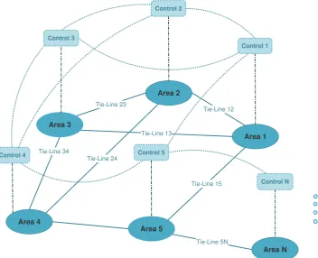
Power system networks can be decomposed into multiple distinct dynamical subsystems, referred to as control areas, each area having two primary characteristics; (1) It comprises of either a single generator or a group of generators, and (2) it maintains a single frequency across its geographical expanse. The areas are responsible for meeting the demand of their own consumers and are interconnected with each other through transmission lines, referred to as tie-lines, over which they exchange certain amount of power normally scheduled over a contracted value for each interconnection. In this paper, we consider a multi-agent representation of power systems where each agent/area has autonomous actuation capacity and is dynamically coupled with certain neighboring agents/areas with which it exchanges state-information. We assume that the topology of the physical links (tie-lines) and the communication scheme coincide. This multi-agent approach to multi-area power systems

links (dotted lines) are incorporated into one unified entity, representing a modern large-scale power

system. The mapping of a cyber network to a physical grid, as shown in Figure1, facilitates the

data-exchange between the control subsystems of interconnected areas and allows for control schemes with distributed architecture. As mentioned earlier, each distinct area consists of a group of generating units, the aggregate power generation of which should match the demand of the consumers spanned across the geographical expanse covered by the corresponding area. The aggregate generation may comprise thermal power stations, hydroelectric plants, wind turbine farms, photovoltaic and battery storage power stations, and, in general, any type of conventional and renewable energy sources. In this work, to avoid further complications in designing distributed control schemes, the power generation of each area is limited to thermal and hydroelectric power stations.

Area 4

Area 3

Area 2

Area 1

Area 5

Area N Tie-Line 23

Tie-Line 12

Tie-Line 34

Tie-Line 5N Tie-Line 13

Tie-Line 24

Tie-Line 15

Control 4

Control 3

Control 2

Control 1

Control N Control 5

Figure 1.Tie-line interconnections (solid lines) and communication scheme (dotted lines) in large-scale multi-area power system.

3.1. Modeling

Let multi-area power system be composed of N areas the topology of which is modeled by

undirected graphG = (V,E). Each nodei ∈ V represents an area and an edge(i,j) ∈ Ebetween

two nodes denotes interaction between the two nodes/areas. We note that the edge(i,j)of the graph

determines coupling terms in the dynamics of areaiandjand also indicates information exchange

between nodei andj. Let also all j ∈ V with j 6= isuch that(i,j) ∈ E be denoted byNi. In the

sequel, allj∈ Niare referred to as adjacent or neighboring nodes/areas toi. At steady-state operation

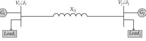
the power sharing via tie-line interconnection between two areasiandjis denoted byPtie,i,jand is

given by:

Ptie,i,j= ViVj

Xij

sin(δi−δj). (1)

Here,Xijis the reactance of the tie-line which connects the two areas,δi,δjrepresent the power

terminals of areaiandj, respectively. Tie-line interconnection in a two-area system is depicted in Figure2.

Vi6 δi Gi

Loadi

Xij

Vj6 δj Gj

Loadj

Figure 2.Tie-line interconnection of two-area system.

For small deviations of(δi,δj)from equilibrium(δ_io,δo_j), the power flow deviation over tie-lineij

from the nominal value is given by the linear equation:

∆Ptie,i,j=Tij(∆δi−∆δj), (2)

where the synchronizing torque coefficient Tij =

|Vi||Vj| Xij cos(δ

o

i −δoj), [10]. Notation ∆ indicates

deviation from steady-state operation conditions; differentiating (2) with respect to time results in:

∆_P˙_tie,i,j =Ktie,i,j ∆fi−∆fj, (3)

whereKtie,i,j=2πTijis referred to as synchronization coefficient between areaiandj, while∆fiand

∆fjrepresent the frequency deviation of each area from their common nominal value, denoted here

by fo_{. According to (3), the linearized dynamics of the total power inflow to thei-th area from all}

interconnected areasj∈ Ni, denoted by∆Ptie,iis given by:

∆_P˙_tie,i=

∑

j∈N_i

Ktie,i,j(∆fi−∆fj). (4)

The open-loop linearized dynamics of thei-th interconnected area is represented by a model

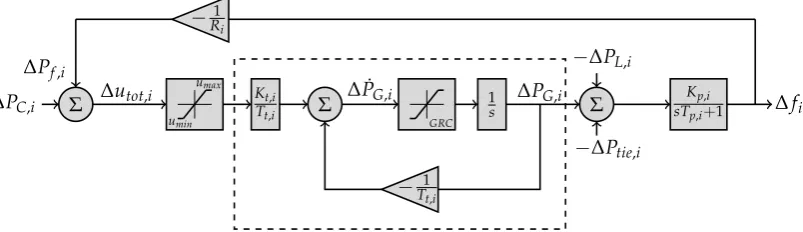
widely used in literature [2,10], the block diagram of which is shown in Figure3.

∆

P

∆

P

Σ

∆

u

∆

P

_Σ

−

∆

P

−

∆

P

K_p,i

sT_p,i+1

∆

f

−

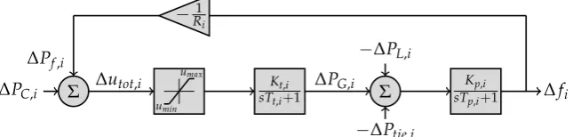
Figure 3.Single block representation of thei-th interconnected area.

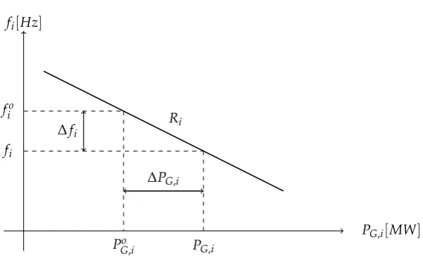
The total control signal of thei-th area is the sum of two components: ∆utot,i = ∆Pf,i+∆PC,i,

namely the primary frequency control action, defined as∆Pf,i =−R1i∆fiand the AGC signal∆PC,ito

be designed. The first is a fixed static linear control law performed by the speed governor which is a regulating unit attached on the prime mover. Detailed description of this topic can be found in [2].

The static gainRiis referred to as speed droop or speed regulation and expresses the ratio of the

frequency deviation∆fito a change in output generated power by∆PG,iassuming the AGC signal

∆PC,i =0. A typical droop characteristic of a single generator actuated by primary frequency control

PG,i[MW] fi[Hz]

Ri

P_Go_,i PG,i f_io

fi

∆fi

∆PG,i

Figure 4.Droop characteristic.

The signal∆utot,iis assumed to be subjected to a component-wise saturation hard constraint of

the form:

∆utot,i,min≤∆utot,i≤∆utot,i,max, (5)

where∆utot,i,max is taken greater than the maximum expected load deviation∆PL,i,max; otherwise,

zero frequency deviation error is not guaranteed. Negative values of∆utot,i allow for handling of

negative values of∆PL,iin case of load reduction. The rate of change of power generation due to the

limitation of the thermal and mechanical movements in the generating unit of each area, as well as the speed governor dead band, are important issues in power system modeling. For simplicity, these constraints will be ignored in the linear stability analysis carried out in Sections4and5, and they will only be considered in simulation results in Section6.

The corresponding state-space form of each area can be written as:

  

∆f˙i

∆P˙G,i

∆P˙tie,i

  =     − 1

Tp,i

Kp,i

Tp,i −

Kp,i

Tp,i

− Kt,i

RiTt,i − 1

Tt,i 0

0 0 0

   

| {z }

A1,i

  

∆fi

∆PG,i

∆Ptie,i

   | {z }

xi

+

∑

j∈Ni

  

0 0 Ktie,i,j(∆fi−∆fj)

  

| {z }

Ei +    0

Kt,i

Tt,i 0

   | {z}

Bu,i ∆PC,i

| {z }

ui

+

  

−Kp,i

Tp,i 0 0

   | {z }

Bw,i ∆PL,i

| {z }

wi

, (6)

fori = 1,· · ·,N, where we have used the state-space differential equations with respect to block

diagram Figure3, along with (4). Note thatEicorresponds to the dynamic coupling between thei-th

area and its adjacent peers and gives rise to a state-space model of non-standard form. A standard state-space model for the complete network will be derived in the sequel. The variables∆fiand∆Ptie,i

in the state-vector have been already defined; variable∆PG,iin (6) is the deviation from equilibrium

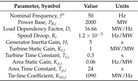
value of the electrical power generated by the aggregate generating units of each area and is taken equal to the mechanical power produced in the output of the turbines. All parameters involved in (6),

along with basic power system terminology, are summarized in Table1. The disturbance signal∆PL,i

denotes time-varying demand of the consumers of thei-th area and is assumed to correspond to

Table 1.Parameters and power system terminology.

Parameter, Symbol Value Units

Nominal Frequency, fo 50 Hz Power Base,PB,i 2000 MW

Load Dependency Factor,Di 16.66 MW/Hz

Speed Droop,Ri 1.2×10−3 Hz/MW

Generator Inertia Gain,Hi 5 s

Turbine Static Gain,Kt,i 1 MW/MW

Turbine Time Constant,Tt,i 0.3 s

Area Static Gain,Kp,i 0.06 Hz/MW

Area Time Constant,Tp,i 24 s

Tie-line Coefficient,Ktie,i 1090 MW/Hz

3.2. State-Augmentation for Integral Action

A well-established technique for tackling step-disturbances with zero steady-state error is to

include integral action into the state-space model. For thei-th area, consider performance variable

expressed as a summation of frequency deviation∆fimultiplied by a bias factorβiand total tie-line

power inflow∆Ptie,i, orzi=βi∆fi+∆Ptie,i. This quantity is referred to as “Area Control Error” (ACE)

and a usual choice for βi isDi+_R1_i, [10]. ParametersDi andRi are defined in Table1. Take now zi=Cz,ixiwithxigiven in (6) andCz,i= [βi0 1]and consider the augmented state-vector:

xa,i=

h

x0_i R zi

i0

. (7)

The augmented state-space form of thei-th area can then be written as:

˙

xa,i =

"

A1,i 03×1

Cz,i 0

#

xa,i+

"

Bu,i

0

#

ui+

"

Ei

0

#

+

"

Bw,i

0

#

wi, (8)

where A1,i,Bu,i,Ei andBw,i are as given in Equation (6). If the coupling termEiin Equation (8) is

neglected, due to state-augmentation by the integral of the ACE signal of each area, a stabilizing

control signaluiwould lead automatically to zero steady-state frequency and tie-line power inflow

deviations provided these are driven by step disturbances wi = ∆PL,i. However the term[E0_i 0]0

involving state-coupling between thei-th area and its neighboring counterparts cannot be neglected,

and therefore the disturbance rejection task for the complete network becomes more challenging.

3.3. Problem Statement

Possible power load change in thei-th area of an interconnected power system causes the electrical

frequency fito deviate from its nominal value. Due to interconnections among the areas through

power transmission tie-lines and the dependence of the power exchange between thei-th andj-th area

upon the respective difference∆fi−∆fj, any power load deviation occurring in thei-th area will also

affect the linkedj-th area, causing a transient alternation in its frequency fj. Here, we formulate the

LFC of multi-area power systems as a large-scale optimal control problem in the absence of state and

input constraints. The special case ofNidentical areas is considered. The aggregate dynamics in this

case can be represented by a state-space model of the form:

˙˜

Here, ˜x= [x0_a,1 · · · x0_a,N], ˜u= [u₁0 · · · u0_N]0, ˜w= [w0₁ · · · w0_N]0and:

A1=

    

−_T1 p

Kp Tp −

Kp Tp 0 − Kt

RTt −

1

Tt 0 0

0 0 0 0

β 0 1 0

    

, A2=

    

0 0 0 0

0 0 0 0

Ktie 0 0 0

0 0 0 0

    

, Bu=

     0 Kt Tt 0 0     

, Bw=

    

−Kp Tp 0 0 0      , (10)

where the subscriptihas been neglected from all entries ofA1,A2,Bu, andBwsince areas are assumed

to have identical dynamics. The LQR design proposed in the next section is presented first from a general multi-agent perspective. This is then extended to the multi-area power system framework.

4. Large-Scale LQR for Dynamically Coupled Systems

Consider a network ofNLdynamically coupled LTI systems referred to as agents. At local level,

the dynamics of thei-th agent is represented in state-space form as:

˙

xi=A1xi+A2

NL

∑

j=1,j6=i

(xi−xj) +Bui,x0,i =xi(0), (11)

wherexi ∈ Rn, ui ∈ Rm are states and inputs of thei-th system, respectively. A complete graph

(with all possible edges)G= (V,E)with Laplacian matrixLcis utilized to model the topology of the

physical links among the agents. Nodei∈ V ofGcorresponds to local statexi, while edge(i,j)∈ E

corresponds to thexi−xjterm in (11). Now construct the aggregate state ˜x∈RnNL_{and input vector}

˜

u∈RmNL_{by stacking all state and input vectors, respectively, of allNLsystems taken in ascending}

order depending on their label in graphG. The aggregate state-space of the network becomes:

˙˜

x =A˜x˜+B˜u˜, ˜x0=x˜(0), (12)

with:

˜

A=INL⊗A1+Lc⊗A2, ˜B=INL⊗B. (13)

Consider now LQR control problem for the network ofNLcoupled systems:

min

˜

u J(u˜, ˜x0)s.t. ˙˜x=

˜

Ax˜+B˜u˜, ˜x0=x˜(0), (14)

where the cost function:

J(u˜, ˜x0) =

Z ∞

0 x˜

0_Q˜x˜+u˜0_{R˜u dt˜ , (15)}

with:

˜

Q=INL⊗Q1+Lc⊗Q2and ˜R=INL⊗R. (16)

Here, the weighting matricesQ1=Q01≥0 andR= R0 >0 penalize local states and inputs of

each node, respectively, while the matrixQ2=Q02 ≥0 is chosen to weigh relative state differences

between subsystems. The following stabilizability and observability assumptions guarantee a solution to LQR problem (14).

Assumption 1. Let C₁0C1=Q1. The pair(A1,B)is stabilizable and(A1,C1)is observable.

Assumption 2. Let C₁₂0 C12 =Q1+NLQ2. The pair(A1+NLA2,B)is stabilizable and(A1+NLA2,C12)

Under Assumption1,2, problem (14) has a unique stabilizing solution ˜u=K˜x˜, which gives finite performance index (15) equal to ˜x0₀P˜x˜0. The optimal state-feedback gain ˜K=−R˜−1B˜0P˜, where ˜Pis the

symmetric positive definite (s.p.d.) solution to the (large-scale) Algebraic Riccati Equation (ARE):

˜

A0P˜+P˜A˜−P˜B˜R˜−1B˜0P˜+Q˜ =0. (17)

Due to special formulation of (14), ˜Kand ˜Pretain certain structure, which will prove essential for designing stabilizing distributed controllers in the next section. The specific structure of these matrices is proved in Theorem1. In the following, we setX=BR−1_B0_.

Theorem 1. Assume P is the s.p.d solution to˜ (17)associated with the optimal solution to(14). Let P˜ ∈

RnNL×nNL _{be decomposed into N}2

L blocks of dimension n×n, each denoted by P˜ij and referred to as the

(i,j)-block ofP. Then, the following statements hold.˜

I. ∑NL

j=1P˜ij =P where P=P0 ≥0is the stabilizing solution to single-node ARE:

A0₁P+PA1−PXP+Q1=0. (18)

II. P˜ij =P˜kl=P˜2for all j6=i, l6=k whereP˜2is symmetric matrix associated with the node-level ARE:

(A1+NLA2)0(P−NLP˜2) + (P−NLP˜2)(A1+NLA2)−(P−NLP˜2)X(P−NLP˜2)

+Q1+NLQ2=0. (19)

Proof. First, we prove part I of the Theorem. The equations corresponding to the diagonal blocks of (17) are:

(A1+ (NL−1)A2)0P˜ii−A02

NL

∑

j=1

j6=i

˜

Pij+P˜ii(A1+ (NL−1)A2)−

NL

∑

j=1

j6=i

˜

PijA2−

NL

∑

k=1

˜

PikXP˜ik

+Q1+ (NL−1)Q2=0, (20)

fori=1,· · ·,NL. Note that ˜Pij=P˜jidue to symmetry of ˜Pin (17). Now let:

Fii=P˜ii+ NL

∑

j=1

j6=i

˜

Pij. (21)

Substituting (21) to (20) gives:

(NL−1)(A20Fii+FiiA2)−NLA02

NL

∑

j=1

j6=i

˜

Pij− NL

∑

j=1

j6=i

˜

PijNLA2 (22a)

+A01(Fii− NL

∑

j=1

j6=i

˜

Pij) + (Fii− NL

∑

j=1

j6=i

˜

Pij)A1−

NL

∑

k=1

˜

PikXP˜ik+Q1+ (NL−1)Q2=0. (22b)

(NL−1)(A02P˜ij+P˜ijA2)−A02(Fii− NL

∑

k=1

k6=i

˜

Pik)−(Fii− NL

∑

k=1

k6=i

˜

Pik)A2−A02

NL

∑

l=1

l6=i l6=j

˜

Pil− NL

∑

l=1

l6=i l6=j

˜

PilA2 (23a)

+A0₁P˜ij+P˜ijA1−

NL

∑

k=1

˜

PikXP˜kj−Q2=0. (23b)

Summing up (23a) for allj6=iblock-wise and adding this summation to (22a) gives:

(NL−1)A02Fii+Fii(NL−1)A2−(NL−1)A02Fii−Fii(NL−1)A2−NLA20

NL

∑

j=1

j6=i

˜

Pij

− NL

∑

j=1

j6=i

˜

PijNLA2+ (NL−1)A02

NL

∑

j=1

j6=i

˜

Pij+ NL

∑

j=1

j6=i

˜

Pij(NL−1)A2+ (NL−1)A02

NL

∑

k=1

k6=i

˜

Pik

+

NL

∑

k=1

k6=i

˜

Pik(NL−1)A2−(NL−1)A02

NL

∑

l=1

l6=i l6=j

˜

Pil− NL

∑

l=1

l6=i l6=j

˜

Pil(NL−1)A2=0 (24)

where all the terms associated withA2cancel out. Summing up (23) over all j 6= iblock-wise and

adding this summation to (22) gives:

A0₁Fii+FiiA1−FiiXFii+ NL

∑

k=1

k6=i

˜

PikX Fii−Fkk

+Q1=0. (25)

Equation (25) has been established in Theorem 1 of [39]. It is true also here due to (24).

Adding up (25) over alli=1,· · ·,NL, we get:

NL

∑

i=1

A0₁Fii+FiiA1−FiiXFii+Q1

=0, (26)

which is sum ofNLidentical ARE’s, i.e.,

NL(A01Fii+FiiA1−FiiXFii+Q1) =0. (27)

Equation (21) impliesFii=∑_iN₌L₁P˜ijwhich, along with (27), proves part I.

Since ˜B, ˜Rare block diagonal and ˜A, ˜Qhave a repetitive pattern, the ARE (17) can essentially be decomposed intoNL identical equations. This implies that all ˜Pijwithi,j=1,· · ·,NLandj6= i

are equal to each other. Let ˜P2 be symmetric matrix representing the off-diagonal blocks ˜Pij of ˜P.

SettingP = Fiifori = 1,· · ·,NL and ˜P2 = P˜ijfori,j =1,· · ·,NL andj 6= iand substituting these

matrices into (23) gives:

(NL−1)A02P˜2+ (NL−1)P˜2A2−A02P−PA2+ (NL−1)A02P˜2+ (NL−1)P˜2A2

−(NL−2)A02P˜2−(NL−2)P˜2A2+A10P˜2+P˜2A1−P˜2X(P−(NL−1)P˜2)

−(P−(NL−1)P˜2)XP˜2−(NL−2)P˜2XP˜2−Q2=0, (28)

(A1+NLA2)0(−NLP˜2) + (−NLP˜2)(A1+NLA2) +NLA02P+PNLA2−(−NLP˜2)XP

−PX(−NLP˜2)−(−NLP˜2)X(−NLP˜2) +NLQ2=0, (29)

or

(A1+NLA2)0(−NLP˜2) + (−NLP˜2)(A1+NLA2) +NLA20P+PNLA2+PXP

−(P−NLP˜2)X(P−NLP˜2)X+NLQ2=0. (30)

Adding now (18) to (30) results in:

(A1+NLA2)0(−NLP˜2) + (−NLP˜2)(A1+NLA2) + (A1+NLA2)0P+P(A1+NLA2)

−PXP+PXP−(P−NLP˜2)X(P−NLP˜2)X+Q1+NLQ2=0, (31)

or

(A1+NLA2)0(P−NLP˜2) + (P−NLP˜2)(A1+NLA2)−(P−NLP˜2)X(P−NLP˜2)

+Q1+NLQ2=0, (32)

which proves part II.

By assumption, the matrices ˜Rand ˜Bare selected block diagonal. Consequently, the state-feedback gain ˜K = −R˜−1B˜0P˜associated with the optimal solution to (14) retains the same structure with ˜P. This leads to the following Corollary.

Corollary 1. AssumeK˜ = −_R˜−1_B˜0_{P is the optimal state-feedback gain obtained from the solution to˜ (14)}

which gives minimum performance indexx˜0₀P˜x˜0withP being the s.p.d solution to˜ (17). LetK˜ ∈RmNL×nNL_and

˜

P∈RnNL×nNL_{be decomposed into N}2

Lblocks of dimension m×n and n×n denoted byK˜ijandP˜ij, respectively each referred to as(i,j)-block of the respective matrix. Then, the following are true;

I. P˜=INL⊗P− Lc⊗P˜2.

II. ∑NL

j=1K˜ij =−R

−1_B0_{P for i=1,· · ·,N}

L.

III. K˜ii=−R−1B0P+ (NL−1)R−1B0P˜2for i=1,· · ·,NL. IV. K˜ij =−R−1B0P˜2for i,j=1,· · ·,NLand j6=i.

V. K˜ =−IN_L⊗R−1B0P+Lc⊗R−1B0P˜2.

Theorem1states that due to special formulation of the cost function (15) and the structure of the

aggregate state-space form (12), the large-scale LQR problem (14) under Assumption1,2can effectively

be reduced to finding the solution of two node-level ARE’s. This feature may be highly beneficial for problems involving networks, the topology of which is modeled by graph with an excessively large number of vertices(NL).

Applying the stabilizing optimal state-feedback control ˜u=K˜x˜to (12) results in a closed-loop matrix, which is Hurwitz and is written as:

Acl= INL⊗(A1−XP) +Lc⊗(A2+XP˜2). (33)

Due to Proposition2, the spectrum ofAclcan be decomposed into:

S(Acl) = NL

[

i=1

whereλc,i ∈ {0,NL,· · ·,NL}.

Remark 1. The matrix A1−XP+αNL(A2+XP˜2)is Hurwitz forα=0andα=1.

In the sequel, we require that:

Condition 1. The matrix A1−XP+αNL(A2+XP˜2)is Hurwitz for allα∈[0, 1].

Condition1states that all convex combinations of two Hurwitz matrices,

µA¯1+ (1−µ)A¯2withµ∈[0, 1], (35)

are Hurwitz, where ¯A1 = A1−XP+NL(A2+XP˜2)and ¯A2 = A1−XP. Sufficient conditions for

Hurwitz stability of convex combination of Hurwitz matrices can be found in Theorem 2.2 in [41].

In essence, Condition1characterizes a class of LQR problems (14) which admit of solutions for which

the Condition1holds. This will be used later for the design of distributed stabilizing controllers.

For a given selection of weighting matrices (Q1,Q2,R) of the LQR problem (14), the validity of

Condition1can be verified by searching for a symmetric positive definite matrix ¯Pfor which the

following LMI,

  

−(A¯0₁P¯+P¯A¯1) 0n×n 0n×n

0n×n −(A¯02P¯+P¯A¯2) 0n×n

0n×n 0n×n P¯

 

>0, (36)

is feasible. Obviously, if matrix ¯P exists then premultiplying and postmultiplying (36) by

[√µIn p1−µIn 0n×n]0 and [√µIn p1−µIn 0n×n], respectively, for µ ∈ [0, 1] leads to

Lyapunov inequality:

(µA¯1+ (1−µ)A¯2)0P¯+P¯(µA¯1+ (1−µ)A¯2)<0, (37)

which admits of a solution ¯P=P¯0>0. This demonstrates thatµA¯1+ (1−µ)A¯2is a Hurwitz matrix

for allµ∈[0, 1]. Alternatively, the stability ofµA¯1+ (1−µ)A¯2can be examined via a simple graphical

test by plotting the eigenvalue with the maximum real part of the matrixµA¯1+ (1−µ)A¯2forµ∈[0, 1].

Distributed LQR Design for Dynamically Coupled Systems

Let sparse network be formed ofNidentical and dynamically coupled LTI systems. We note here

that the indexNdiffers fromNLemployed for networks modeled by complete graph in the previous

section, and in the sequel, we use indexNto refer to schemes with sparse structure. Let the couplings

among the systems be modeled by graphGN= (V,E)with Laplacian matrixLN. The neighborhood

of thei-th system is denoted byN_i ⊂ Vand comprises allj∈ Vwithj6=i, for which(i,j)∈ E. Let the dynamics at local level of thei-th system be:

˙

xi =A1xi+A2

∑

j∈Ni

(xi−xj) +Bui,x0,i=xi(0), (38)

wherexi ∈Rnandui ∈Rm. The aggregate state-space of the network becomes:

˙˜

x =A˜x˜+B˜u˜, ˜x0=x˜(0), (39)

where ˜x ∈RnN, ˜u∈RmN and:

˜

Note that the Laplacian matrixLNin (40) does not necessarily correspond to a complete graph

in contrast to (13) and generically the matrix ˜Ain (40) is sparse. A stabilizing distributed controller for (39) is constructed in the following Theorem. For convenience, we setX=BR−1B0.

Theorem 2. Consider a network of N coupled systems with dynamics described in(38). The network topology is modeled by graphGNwith Laplacian matrixLN. LetλNbe the maximum eigenvalue ofLNand denote by dmax the smallest integer which is greater than or equal toλN. Consider LQR problem(14)for NL =dmax, define P andP˜2via(18)and(19), respectively, and assume Condition1is true. Define also distributed state-feedback gain:

ˆ

K=−IN⊗R−1B0P+LN⊗R−1B0P˜2. (41)

Then, the closed-loop matrix,

Acl= IN⊗(A1−XP) +LN⊗(A2+XP˜2), (42)

is Hurwitz.

Proof. Consider the spectrum S(Acl) = S(IN⊗(A1−XP) +LN⊗(A2+XP˜2)). LetVN⊗In be

state-space transformation, whereVN ∈ RN×N is an orthogonal matrix whose columns consist of

the eigenvectors ofLN. In the transformed coordinates, ¯Acl = IN⊗(A1−XP) +ΛN⊗(A2+XP˜2),

whereΛN=diag(0,λ2,· · ·,λN)withλN ≤dmax. The spectrum of ¯Aclis:

S(A¯cl) = N

[

i=1

(A1−XP+λi(A2+XP˜2)), (43)

whereλifori=1,· · ·,Nare the eigenvalues ofLN. Condition1holds, hence(A1−XP) +αdmax(A2+

XP˜2) is Hurwitz for all α ∈ [0, 1]. Consequently, ¯Acl is also Hurwitz since λi ∈ [0,dmax] for all i=1,· · ·,N. This proves the Theorem.

Remark 2. For a time-varying graph G(t) = (V,E(t)) with fixed number of vertices (N) and time-varying edges the maximum eigenvalue of the time-varying Laplacian matrixL(t)is bounded by2N. Consequently, solving(14)for NL=2N and assuming Condition1holds leads to a distributed controllerK,ˆ which stabilizes the network for all possible couplings among the N systems. Naturally, this does not imply stability of switching between stable network interconnections.

5. Large-Scale LQR for LFC

In this section, we consider LQR problem (14) for a multi-area power system. Recall that we

denote byNLthe number of areas of power network, the topology of which is modeled by complete

graph and byNthe number of areas corresponding to sparse networks. Let the aggregate state-space

model ofNL-area power system be written as:

˙˜

x= (INL⊗A1+Lc⊗A2)x˜+ (INL⊗Bu)u˜+ (INL⊗Bw)w˜, (44)

where ˜x = [x0_a,1 · · · x0_a,NL], ˜u = [u₁0 · · · u0_NL]0, ˜w = [w0₁ · · · w0_NL]0 withxa,i,ui,wifori =1,· · ·,NL

defined in (8) and:

A1=

     −1 Tp Kp Tp −

Kp Tp 0 − Kt

RTt −

1

Tt 0 0

0 0 0 0

β 0 1 0

    

, A2=

    

0 0 0 0

0 0 0 0

Ktie 0 0 0

0 0 0 0

    

, Bu=

     0 Kt Tt 0 0     

, Bw=

    

Parameters in(A1,A2,Bu,Bw)can be found in Table1. In view of Assumption1, LQR problem (14)

for ˜A = INL ⊗A1+Lc⊗A2 and ˜B = INL⊗Bu with (A1,A2,Bu) given in (45) initially fails to

admit a solution since (18) cannot be solved. This stems from the fact that the pair (A1,Bu)has

an uncontrollable mode at the origin, and the realization (44) is non-minimal. The non-minimality is due to a redundant equation related to the sum of the total power inflow∆Ptie,ito each area, which

equals zero or∑NL

i=1∆Ptie,i = 0. Now, we show how to reformulate the system matrices and derive

a stabilizing controller for the network. Define permutation matrix:

T=     

1 0 0 0

0 1 0 0

0 0 0 1

0 0 1 0

     , (46)

where T = T0 = T−1 and consider Kalman decomposition of the pair (A1,Bu) applying

state-space transformation Txa,i for i = 1,· · ·,NL. Let the system matrices (A¯1, ¯A2, ¯Bu, ¯Bw) =

(TA1T0,TA2T0,TBu,TBw)in the new coordinates be written as:

¯

A1=

     −1 Tp Kp

Tp 0 − Kp Tp − Kt

RTt −

1

Tt 0 0

β 0 0 1

0 0 0 0

    

, ¯A2=

    

0 0 0 0

0 0 0 0

0 0 0 0

Ktie 0 0 0

    

, ¯Bu=

     0 Kt Tt 0 0     

, ¯Bw=

    

−Kp Tp 0 0 0      , (47)

where ¯Bu=Bu, ¯Bw =Bw. The controllable part of(A¯1, ¯Bu)is denoted by(Ac,Bc)with:

Ac=

  

−_T1 p

Kp Tp 0 −Kt

RTt −

1

Tt 0

β 0 0

  , Bc=

   0 Kt Tt 0  

. (48)

The zero in the(4, 4)entry of ¯A1stands for the uncontrollable mode at the origin of(A1,Bu).

Now, construct perturbation matrix:

E=

"

03×3 03

0₃0 e

#

, (49)

fore<0 with|e|sufficiently small and define:

A1e= A¯1+E=

"

Ac A12

00₃ e

#

, A2e =A¯2− 1

NLE

=

"

03×3 03

a21 −_N1_Le

#

, (50)

where A12 = [−RTKtt 0 1]

0 _{and a}

21 = [Ktie 0 0]. Since e < 0, the pair (A1e,Bu) is stabilizable.

According to Theorem1, LQR problem (14) with parameters(A1e,A2e,Bu,Q1,Q2,R)is reduced to two

node-level ARE:

A0_1ePe+PeA1e−PeXPe+Q1=0, (51)

(A1e+NLA2e)0(Pe−NLP˜2e) + (Pe−NLP˜2e)(A1e+NLA2e)−(Pe−NLP˜2e)X(Pe−NLP˜2e)

+Q1+NLQ2=0, (52)

wherePe, ˜P2earee-dependent andX=BuR−1B0u. Note that the solutionPe−NLP˜2eto ARE (52) remains

invariant undere-perturbation. Theorem3, next, summarizes the method of solving large-scale LQR

Theorem 3. Consider NL-area power system with aggregate state-space form given as in(44). Consider Kalman decomposition of (A1,Bu) and define (A¯1, ¯A2, ¯Bu, ¯Bw)given in (47). Choose e < 0with |e| sufficiently small and define perturbed matrices A1e, A2e as given in(50). Solving LQR problem(14)with parameters

(A1e,A2e,Bu,Q1,Q2,R) and defining Pe and P˜2e from(51) and(52), respectively, leads to the following argument: the matrix,

¯

A1−XPe+α(NLA¯2+XP˜2e), (53)

I. is Hurwitz forα=1.

II. has n−1eigenvalues in the left-half-plane and one at the origin forα=0.

Proof. In view of the special structure ofA1eandA2e, it can easily be seen that:

¯

A1+NLA¯2=A1e+NLA2e. (54)

Due to (52), the matrixA1e+NLA2e−XPe+NLXP˜2eis Hurwitz and because of (54) the matrix

¯

A1+NLA¯2−XPe+NLXP˜2eis also Hurwitz. This proves part I.

Now, let the matrixPein (51) be decomposed into blocks of appropriate dimensions according to

the Kalman decomposition (48). Then, ARE (51) can be written as:

"

Ac A12

00₃ e

#0"

P11e P12e P₁₂0 _e P22e

#

+

"

P11e P12e P₁₂0 _e P22e

# "

Ac A12

00₃ e

#

−

"

P11e P12e P₁₂0 _e P22e

# "

Bc

0

#

R−1hB0c 0

i "

P11e P12e P₁₂0 _e P22e

#

+

"

Q11 Q12

Q0₁₂ Q22

#

=0. (55)

The first diagonal block of (55) gives:

A0_cP11e+P11eAc−P11eBcR−1B0cP11e+Q11 =0, (56)

and implies that the matrixAc−BcR−1Bc0P11eis Hurwitz where the symmetric positive definite matrix P11edoes not depend on parametere. The two remaining blocksP12eandP22eofPearee-dependent

and given by:

P12e =−(A0c−P11eBcR−1Bc0+eIn−1)−1(P11eA12+Q12), (57)

P22e = 1

2e[(P

0

12eBcR−1Bc0−2A012)P12e−Q22]. (58)

The matrixA0c−P11eBcR−1B0c+eIn−1in (57) is invertible sinceAc−BcR−1Bc0P11e is Hurwitz and e<0. Now, the closed-loop matrixA1e−BuR−1B0uPeis Hurwitz and can be written as:

A1e−BuR−1B0uPe=

"

Ac−BcR−1B0cP11e A12−BcR−1B0cP12e

00₃ e

#

. (59)

Since (59) is in canonical form, its spectrum can be decomposed in:

S(A1e−BuR−1Bu0Pe) =S(Ac−BcR−1Bc0P11e)∪e. (60)

Settinge=0 in (60) proves the Theorem.

Similarly to Condition1, we impose the following stability requirement.

In the next paragraph, we propose distributed stabilizing LFC controllers for multi-area power

systems with sparse topology based on Condition2.

5.1. Distributed LQR-Based LFC

Let undirected graphG_N = (V,E)with Laplacian matrixL_N(G_N)models the interconnection

topology of a multi-area power system formed ofNidentical areas with aggregate state-space form

written as:

˙˜

x= (IN⊗A1+LN⊗A2)x˜+ (IN⊗Bu)u˜+ (IN⊗Bw)w˜. (61)

The matricesA1, A2, Bu, andBw are given as in (45). The aggregate vectors ˜x, ˜u, and ˜ware

constructed by stacking the augmented state-vectorxa,i, input-vectorui, and disturbance-vectorwi,

respectively, shown in (8) of each area with ascending order depending on graphGN. Now, define

perturbation matrix:

E=

    

0 0 0 0

0 0 0 0

0 0 e 0

0 0 0 0

    

, (62)

wheree<0 and|e|sufficiently small, and also define perturbed matricesA1eandA2eas:

A1e= A1+E, A2e= A2− 1

NLE, (63)

whereNL is as defined in Theorem2. A distributed LFC controller for (61) is constructed next, in

Theorem4.

Theorem 4. Consider power system of N identical areas with network topology modeled by graphG_Nwith Laplacian matrixLNand aggregate state-space form given by(61). LetλNbe the maximum eigenvalue ofLN and denote by dmax the smallest integer which is greater than or equal toλN. Set NL =dmax, specify e<0 with|e|sufficiently small and define perturbed matrices A1eand A2e as in(63). Consider LQR problem(14) for NL =dmax perturbed systems(A1e,A2e,Bu), define PeandP˜2evia(51)and(52), respectively, and assume Condition2holds. Define also distributed state-feedback gain:

ˆ

K=−IN⊗R−1B0uPe+LN⊗R−1Bu0P˜2e. (64)

Then, the closed-loop matrix of the original system,

Acl =IN⊗(A1−XPe) +LN⊗(A2+XP˜2e), (65)

has3N−1eigenvalues in the left-hand-plane and one at the origin.

The proof follows similar arguments stated for proving Theorem 2 and is omitted here.

The conclusions as far as the stability of the network is concerned still hold, even if the controllability

Assumption1is no longer valid. The distributed state-feedback gain (64) can be used for stabilizing

the network despite the fact that the closed-loop matrix (65) has a single eigenvalue at the origin.

This mode corresponds to the trivial differential equation∑NL

i=1∆P˙tie,i =0, which implies ˙0=0 and

can be easily derived via an appropriate state-space transformation.

are beyond the scope of this paper. Nonlinearities and parameter perturbations considered in the next section are only used for simulation purposes where the performance of the proposed control scheme is also tested under more intense conditions.

6. Simulation Case Studies

We consider a power system of six identical areas, the parameters of which are summarized

in Table1. Three interconnection schemes are considered; each graph shown in Figure5a–c, with

corresponding Laplacian matrix given in (66), models the network topology of one of the three schemes (S1,S2,S3), respectively.

1 2

3

4 5

6

(a) Interconnection schemeS1 with Laplacian matrixL1.

1 2

3

4 5

6

(b) Interconnection schemeS2 with Laplacian matrixL2.

1 2

3

4 5

6

(c) Interconnection schemeS3 with Laplacian matrixL3.

Figure 5.Three different tie-line interconnection schemes of six control areas.

L1=

        

2 −1 0 0 −1 0

−1 2 −1 0 0 0

0 −1 3 −1 0 −1 0 0 −1 2 −1 0

−1 0 0 −1 2 0

0 0 −1 0 0 1         

,L2=

        

1 0 0 0 −1 0 0 1 −1 0 0 0 0 −1 2 −1 0 0 0 0 −1 3 −1 −1

−1 0 0 −1 2 0

0 0 0 −1 0 1         

,L3=

        

3 0 −1 0 −1 −1 0 1 0 −1 0 0

−1 0 1 0 0 0

0 −1 0 2 −1 0

−1 0 0 −1 3 −1

−1 0 0 0 −1 2

         . (66)

In the simulations, one scenario is considered in which the areas are assumed to be subjected to step disturbances. These represent power load variations of the consumers of each area and

are depicted in Figure6. For the control design, we also assume that there is a communication

cyber-layer, the topology of which is identical with this of the tie-line interconnection scheme

considered. The distributed LFC controller designed in Theorem4was tested in three case studies,

which are summarized below:

1. We test closed-loop stability of topologyS1,S2, andS3, respectively, applying LFC controller

derived by solving a single LQR problem. This stability test is performed for two different tunings of the LQR performance index. The transients of frequency and total power inflow of the linear model of each area is compared to the corresponding responses, including saturation hard constraint on the total input signal of each area.

2. We consider parametric uncertainty in the linear model of each area, and we show closed loop

stability of topologyS2for two different tunings of the LFC controller. Perturbations have been

carried out on the following parameters: turbine time constant(Tt,i), area time constant(Tp,i)of

each area, respectively, and tie-line coefficient(Ktie,i,j)of each tie-line interconnection.

3. For a certain tuning of the LFC controller, we demonstrate frequency recovery for topologyS1,S2,

andS3, respectively, including generation rate constraint (GRC) and saturation hard constraint on

the total input signal of each area.

6.1. Case Study 1

corresponds to one of those given in (66) according to the topology considered. Parameter values are

given in Table1. The distributed LQR controller presented in Section5.1is proposed here to drive the

AGC signal∆PC,iof each area. The control objective is to meet the load demand at each area shown in

Figure6and recover the nominal operating conditions of each area for three possible interconnections.

Stabilizing distributed state-feedback controller is constructed as follows.

0 5 10 15 20 25 30 35 Time [sec]

-200 -150 -100 -50 0 50 100 150 200

P

L,i

[MW]

Disturbance Profiles

area 1 area 2 area 3 area 4 area 5 area 6

Figure 6.Power demand deviation∆PL,ifori=1,· · ·, 6.

0 0.1 0.2 0.3 0.4 0.5 0.6 0.7 0.8 0.9 1 -4

-3.5 -3 -2.5 -2 -1.5 -1 -0.5 0

magnitude

max real part of eig(A

1+BuK+ 5(A2+BuK2)

Q 2=200Q1 Q

2=0

Figure 7.Stability test and validity of Condition2.

The maximum eigenvalue of each matrix (L1,L2,L3) in (66) is 4.3028, 4.3028, and 4.3928,

respectively. We take the smallest integer denoted bydmaxwhich is greater or equal to the maximum of

these (4.3928), i.e.,dmax =5. We select perturbation parametere=−0.01, and we alter matricesA1and

A2toA1eandA2e, respectively, according to (63). We solve optimal problem (14) forNL =dmax =5

systems with matrices (A1e,A2e,Bu)for two different selections of the weights ˜Q, ˜R. In the first,

˜

Q= I5⊗Q1, withQ1=diag(100, 10, 10, 5000)and ˜R= I5⊗100, while in the second, ˜Ris kept the

same and ˜Q= I5⊗Q1+L5⊗Q2, whereQ2=200Q1andL5is Laplacian matrix corresponding to

complete graph (all possible edges) with 5 nodes. The matrixQ2penalizes the relative state-difference

(xi−xj) between neighboring areas in (15). We evaluatePeand ˜P2efrom (51), (52), and we define the

respectiveK=−R−1_B0

uPeandK2=R−1B0uP˜2estate-feedback gains for each tuning. These are:

K=h−2502.857 −1.203 −1.757 −7.071i

K2=

h

−342.491 −0.104 0.225 0.000i

(67)

K=h−2502.857 −1.203 −1.757 −7.071i

K2=

h

−12084.071 −2.356 −6.374 −43.329i

(68)

for the case whereQ2 = 200Q1. Note that K = −R−1Bu0Pe is the same for both cases since Pe is

the solution to a single node-level ARE with parameters(A1e,Bu,Q1,R). We also test the validity of

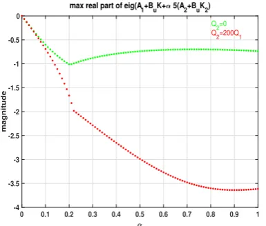
Condition2, which can be seen to hold. Figure7displays the real part of the eigenvalue of the matrix

(A1−BuR−1Bu0Pe) +αdmax(A2+BuR−1B0uP˜2e) with the maximum real part withα ∈ [0, 1]for both

tuning choices. In essence, this implies stable operation of the network under both control schemes for all possible interconnections corresponding to Laplacian matrices with maximum eigenvalue bounded bydmax.

At network level, the distributed stabilizing controller ˆKtakes the form:

ˆ

K= I6⊗K+Ls⊗K2, (69)

whereLs,s=1, 2, 3, is given in (66) according to the topology. Node-wise, the AGC signal at each area

is derived from:

∆PC,i=Kxi+K2

∑

j∈N_i

(xi−xj), (70)

withi=1,· · ·, 6,j6=iandj∈ N_i. In effect, each area requires local state and state-information from its neighboring areas be accessible for measuring in order to construct its control signal. In the following simulations, we show the transients of frequency and total power inflow of each area resulting from

the corresponding power demand deviation∆PL,i,i= 1,· · ·, 6 of each area. Comparison with the

response of the corresponding model of each area which includes saturation hard constraint on the total input signal of each area is also illustrated in the simulation results. Block representation of each

area with saturating input constraint is shown in Figure8, where the symmetric saturator models the

lower and upper bound of the magnitude of the total control signal of each area. Here, we consider

−220[MW]≤∆utot,i ≤220[MW],i=1,· · ·, 6.

∆PC,i

∆Pf,i

Σ ∆utot,i

umin umax

K_t,i sTt,i+1

∆PG,i _Σ

−∆Ptie,i −∆PL,i

K_p,i

sTp,i+1 ∆fi −1

Ri

Figure 8.Single block representation of thei-th interconnected area with saturation hard constraint on the total input signal.

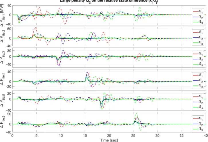
Figures 9–12 show the transient response of frequency and total power inflow deviation,

respectively, of each area from the equilibrium operation for two control schemes given in (67), (68). Stable operation is guaranteed and the nominal working conditions for all three interconnection schemes are recovered via both LFC control choices. For the given choices of weighting matrices (Q1,Q2,R), this is guaranteed from the validity of Condition2, which was checked graphically in

Figure7. Note also, the magnitude of the total power flow over the tie-lines is significantly limited

in the case where the controller is designed as in (68). This stems from the large weighting matrix

Q2selection in the performance index (15). In this case, since the relative state-difference between

neighboring areas is highly penalized, the areas tend to acquire same frequencies deviations during

the transients (see Figure11), thus the total power flow over the tie-lines given in (4) is kept low.

Comparing Figures10and12, the same behavior is observed for the case in which saturating input

(xi−xj)is penalized heavily in the LQR performance index. This powerful feature to control the

magnitude of tie-line power exchange enhances the applicability of the proposed controller and might prove highly beneficial for networks composed of weak tie-line interconnections.

Figure 9.Frequency transients of the six-area power system for three tie-line interconnection schemes

(S1,S2,S3). Zero penalty on the relative state-difference between interconnected areas. Solid lines depict transients of the linear model; dashed lines depict transients of the model with saturator (Figure8).

Figure 11.Frequency transients of the six-area power system for three tie-line interconnection schemes

(S1,S2,S3). Large penalty on relative state-difference between interconnected areas. Solid lines depict transients of the linear model; dashed lines depict transients of the model with saturator (Figure8).

Figure 12.Total power inflow response of the six-area power system for three tie-line interconnection schemes(S1,S2,S3). Large penalty on relative state-difference between interconnected areas. Solid lines depict transients of the linear model; dashed lines depict transients of the model with saturator (Figure8).

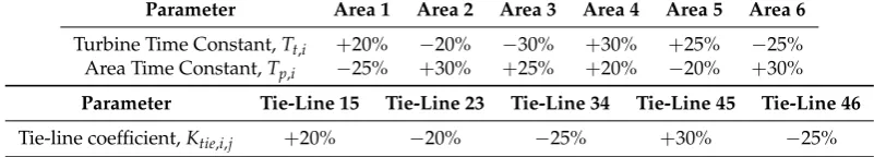
6.2. Case Study 2

the interconnection topologyS2shown in Figure5b. Both tunings of the LQR performance index

considered in the previous section are also employed here. We consider parametric uncertainties in: turbine time constantTt,i, area time constantTp,iand tie-line coefficientKtie,i,jfori,j=1,· · ·, 6 and

j∈ Ni. The perturbation magnitude of each parameter is shown in Table2.

Table 2.Parametric uncertainties inTt,i,Tp,iandKtie,i,j,i=1,· · ·, 6,j∈ Ni.

Parameter Area 1 Area 2 Area 3 Area 4 Area 5 Area 6

Turbine Time Constant,Tt,i +20% −20% −30% +30% +25% −25%

Area Time Constant,Tp,i −25% +30% +25% +20% −20% +30%

Parameter Tie-Line 15 Tie-Line 23 Tie-Line 34 Tie-Line 45 Tie-Line 46

Tie-line coefficient,Ktie,i,j +20% −20% −25% +30% −25%

The frequency and total power inflow deviation of each area driven by step disturbances (Figure6)

are depicted in Figures13–16. The robustness of the proposed distributed LQR-based LFC scheme is

validated, and it can be seen that stable operation is maintained even for magnitude of parametric uncertainties taken equal to 30%.

0 5 10 15 20 25 30 35

Time [sec]

-0.15 -0.1 -0.05 0 0.05 0.1

Frequency

fi

[Hz] - Topology S

2

Zero Penalty Q₂ on |x_i-x_j| - Topology S₂

area 1 area 2 area 3 area 4 area 5 area 6

Figure 13.Frequency deviation∆firesponse fori=1,· · ·, 6, topologyS2, control tuning withQ2=0, uncertain parameters.

0 5 10 15 20 25 30 35

Time [sec]

-0.08 -0.06 -0.04 -0.02 0 0.02 0.04 0.06

Frequency

fi

[Hz] - Topology S

2

Large Penalty Q₂ on |x_i-x_j| - Topology S₂

area 1 area 2 area 3 area 4 area 5 area 6

0 5 10 15 20 25 30 35 Time [sec]

-80 -60 -40 -20 0 20 40 60 80 100

Power inflow

P

tie,i

[MW] - Topology S

2

Zero Penalty Q₂ on |x_i-x_j| - Topology S₂

area 1 area 2 area 3 area 4 area 5 area 6

Figure 15.Total power inflow deviation∆Ptie,iresponse fori=1,· · ·, 6, topologyS2, control tuning withQ2=0, uncertain parameters.

0 5 10 15 20 25 30 35

Time [sec]

-20 -15 -10 -5 0 5 10 15 20 25

Power inflow

P

tie,i

[MW] - Topology S

2

Large Penalty Q₂ on |x_i-x_j| - Topology S₂ area 1 area 2 area 3 area 4 area 5 area 6

Figure 16.Total power inflow deviation∆Ptie,iresponse fori=1,· · ·, 6, topologyS2, control tuning withQ2=200Q1, uncertain parameters.

6.3. Case Study 3

In this simulation study, the linear model of each area is augmented by saturation hard constraint on the total control signal and generation rate constraint (GRC). The first is formulated as hard input constraint and is taken equal to this considered in the first case study,−220[MW]≤∆utot,i ≤220[MW], i=1,· · ·, 6. The second constraint (GRC) can be cast as state constraint imposed on the state variable ∆PG,i,=1,· · ·, 6. Here, we consider GRC equal to 10% of the power base of each area per minute

(i.e., 3.4 [MW/s]). The augmented block diagram of each area is depicted in Figure17.

∆PC,i

∆Pf,i

Σ ∆utot,i

umin umax

Kt,i T_t,i Σ

GRC

1

s

− 1

Tt,i

∆_P˙_{G,i ∆PG,i} Σ

−∆Ptie,i −∆PL,i

Kp,i

sT_p,i+1 ∆fi −1

Ri

Each area is subjected to step disturbances shown in Figure6. The three tie-line interconnection schemes depicted in Figure5are considered in the simulations. In this case study, in order to construct the proposed LFC controller, the weighting matrices of the LQR performance index have been chosen according to Bryson’s rule [45]. For a standard LQR problem with weights(Q,R), this rule specifies

thatQandRare taken diagonal with diagonal entries defined as:

Qii=

1 (xi,max)2

andRii=

1 (ui,max)2

, (71)

where|xi,max|and|ui,max|represent the maximum required values of the state and control variables,

respectively. Here, the matrices(Q1,Q2,R)are selected as: Q1 = diag(_0.0011 2,₄₅₀12,₂₀₀12,₁₀₀12),Q2 =

diag(_0.112,₅₀12,₄₀₀12,₅₀₀₀1 2)andR = 10000₃₅₀2 . The frequency transient of the closed-loop system of each

area is illustrated in Figure18.

Figure 18.Frequency transients of the six-area power system for three tie-line interconnection schemes

(S1,S2,S3). Input and state constraints are included in the model of each area (Figure17). Selection of weighting matrices according to Bryson’s rule.

As it can be seen, the same LFC controller stabilizes the network for topologyS1,S2, andS3

and nominal frequency for each area is recovered. The frequency transient in this case has become considerably slower than in previous studies due to the state constraint GRC, which significantly limits the rate of power generation (3.4 [MW/s]). Despite the strong nonlinearities introduced by the input and state constraint, the closed-loop stability is maintained via the proposed LFC controller.

7. Conclusions

system areas. First, a fully centralized controller was designed which was subsequently substituted by a distributed state-feedback gain with sparse structure. The control scheme was obtained by optimizing an LQR performance index with a tuning parameter utilized to emphasize/de-emphasize relative state difference between interconnected areas. We showed that this parameter controls the magnitude of tie-line power exchange and frequency synchronization between interconnected areas. Our approach enhances power system modularity and leads to a simple and verifiable stabilizability condition for a class of network topologies. Extensive simulations presented in this work support our conjecture that this stabilization criterion can be extended to more general LFC control network problems. The assumption of identical dynamics is clearly restrictive but simplifies the design problem considerably and leads to the derivation of a stability condition which can be easily tested. Attempts to eliminate or relax this assumption will be the topic of future work. Preliminary results

in this direction can be found in [42,43]. The simulation results in Section6.2 carried out under

considerable perturbations suggest that this hypothesis is valid and that our results can be extended to the non-identical case.

Author Contributions: All authors have contributed equally to the derivation of the results of this work. All authors have approved the publication of this paper.

Funding:L. Dritsas acknowledges financial support from the Special Account for Research of ASPETE through the funding program “Strengthening research of ASPETE faculty members”.

Conflicts of Interest:The authors declare no conflict of interest.

References

1. Iracleous, D.P.; Alexandridis, A.T. A multi-task automatic generation control for power regulation.

Electr. Power Syst. Res.2005, doi:10.1016/j.epsr.2004.06.011. [CrossRef]

2. Kundur, P.Power System Stability And Control; McGraw-Hill, Inc.: London, UK, 1993.

3. Tielens, P.; Van Hertem, D. The relevance of inertia in power systems. Renew. Sustain. Energy Rev.2016, 55, 999–1009, doi:10.1016/j.rser.2015.11.016. [CrossRef]

4. Ulbig, A.; Borsche, T.S.; Andersson, G. Impact of low rotational inertia on power system stability and operation.IFAC Proc. Vol.2014,47, 7290–7297. [CrossRef]

5. Masood, N.A.; Modi, N.; Yan, R. Low inertia power systems: Frequency response challenges and a possible solution. In Proceedings of the 2016 Australasian Universities Power Engineering Conference (AUPEC), Brisbane, Australia, 25–28 September 2016. doi:10.1109/AUPEC.2016.07749335.

6. Tielens, P.; van Hertem, D. Grid Inertia and Frequency Control in Power Systems with High Penetration of Renewables. In Proceedings of the Young Researchers Symposium in Electrical Power Engineering, Delft, The Netherlands, 16–17 April 2012.

7. Žertek, A.; Verbiˇc, G.; Pantoš, M. A novel strategy for variable-speed wind turbines’ participation in primary frequency control. IEEE Trans. Sustain. Energy2012,3, 791–799, doi:10.1109/TSTE.2012.2199773. [CrossRef] 8. Attya, A.B.T.; Hartkopf, T. Control and quantification of kinetic energy released by wind farms during power system frequency drops. IET Renew. Power Gener.2013,7, 210–224, doi:10.1049/iet-rpg.2012.0163. [CrossRef]

9. Oshnoei, A.; Khezri, R.; Muyeen, S.; Blaabjerg, F. On the Contribution of Wind Farms in Automatic Generation Control: Review and New Control Approach.Appl. Sci.2018,8, 1848, doi:10.3390/app8101848. [CrossRef]

10. Bevrani, H.Robust Power System Frequency Control; Springer: Berlin/Heidelberg, Germany, 2010.

11. Ma, J. Power System Wide-Area Stability Analysis and Control; Wiley: Hoboken, NJ, USA, 2018; doi:10.1002/9781119304852.

12. Shayeghi, H.; Shayanfar, H.A.; Jalili, A. Load frequency control strategies: A state-of-the-art survey for the researcher. Energy Convers. Manag.2009, doi:10.1016/j.enconman.2008.09.014. [CrossRef]