The quantum free electron laser

The Quantum Free-Electron Laser

Gordon R.M. Robb

University of Strathclyde & Scottish Universities Physics Alliance (SUPA), John Anderson Building, 107 Rottenrow, Glasgow, G4 0NG, UK

Abstract

The quantum regime of the free-electron laser (FEL) interaction, where the recoil associated with photon emission plays a significant role, is discussed. The role of quantum effects and their relation to electron beam coherence are considered. An outline derivation of a 1D quantum high-gain FEL model and some of its predictions for the behaviour of a quantum FEL in the linear and non-linear regimes are presented. The effect of slippage and, consequently, the quantum regime of self-amplified spontaneous emission are discussed. Sug-gestions on how to realise a quantum FEL are presented and some recent re-lated work is summarized.

Keywords

Free-electron laser; quantum; recoil.

1 Introduction

Free-electron lasers (FELs) have demonstrated the ability to produce coherent radiation ranging from the microwave to the X-ray region of the electromagnetic spectrum. Although the first theoretical studies of the FEL involved a quantum mechanical analysis (e.g., [1]), it is generally accepted that FEL experiments

to dateare well described by classical models in which an electron beam consisting of classical particles interacts with a classical electromagnetic radiation field. Until relatively recently, most theoretical studies using a quantum analysis have been restricted to the regime of low gain (e.g., [2–6]). More recently, however, there has been a revival of interest in the role of quantum effects in the FEL interaction (e.g., [7–9]), stimulated in part by the development of short-wavelength, high-gain FEL amplifiers producing progressively higher-energy photons (see, e.g., Ref. [10] for a review of X-ray FELs). In this article, methods for describing the quantum regime of high-gain FEL operation are outlined and some of the effects which are beyond description by the usual classical models are discussed.

2 The role of quantum effects in the free-electron laser interaction 2.1 Recap of classical high-gain free-electron laser theory

In this section, a brief summary of 1D classical high-gain FEL theory is presented, which will be used both as a benchmark with which to compare the results from the quantum model, and to illustrate where the limitations of classical FEL models occur.

Classical high-gain FEL models (e.g., [11–13]) describe the self-consistent evolution of a collec-tion of relativistic electrons interacting with an electromagnetic radiacollec-tion field as they propagate through an undulator/wiggler magnet. The Newton–Lorentz equations of motion describing the dynamics of each electron and Maxwell’s wave equation can be written in a dimensionless, universally scaled form where the number of free parameters is minimized [11]:

dθj

d¯z = ¯pj , (1)

d¯pj

d¯z = −

¯

d ¯A

d¯z = D

e−iθE+ iδA ,¯ (3)

whereθj = (k+kw)z−ωtj is the electron ponderomotive phase,pj¯ = (γj−γr)/ργris the scaled en-ergy/momentum change of each electron,z¯=z/Lgis the scaled position in the wiggler,Lg =λw/4πρ is the gain length,δ= (γ0−γr)/ργris the scaled detuning of the beam energy from its resonance value, whereγ0 is the initial Lorentz factor of the electron beam,γris the Lorentz factor of the electron beam at resonance, which satisfies the FEL resonance conditionγr =

p

λw(1 +a2w)/2λ, whereλis the radi-ation wavelength andaw =eBw/mckwis the wiggler deflection parameter for a wiggler with magnetic field, Bw, and wiggler wavenumber, kw = 2π/λw, whereλw is the wiggler period. The dimension-less radiation field amplitude_A¯_{is defined so that|A}¯_|2 ₌

0|E|2/ρ~ωne, where|E|is the electric field amplitude,ne is the electron beam density,k = 2π/λis the wavenumber of the radiation,ω = ckis the angular frequency of the radiation andcis the speed of light. The average,h(...)i ≡ _N1 PNj=1(...)j,

wherej = 1, . . . , N is the electron index, andN is the number of electrons. The FEL parameterρis

defined as

ρ= 1

γr

awωp 4ckw

2/3

, (4)

whereωp =

p e2_n

e/0mis the plasma frequency associated with the electron beam,mis the electron mass, andeis the magnitude of the electron charge. In deriving Eqs. (1)–(3), the relative slippage of the radiation with respect to the electron beam has been neglected.

Assuming an initial condition corresponding to equally distributed electron phases, a monoener-getic electron beam, and no electromagnetic field, i.e.,

D

e−iθE= 0, p¯j = 0∀j, A¯= 0,

then a linear stability analysis [11] shows that this initial condition is unstable to fluctuations in the electromagnetic field amplitude and electron phase, i.e., shot noise. A numerical solution of Eqs. (1)–(3) with initial conditions _D

e−iθE= 0, pj¯ = 0∀j , |A¯|= 10−4, δ= 0

is shown in Fig. 1, showing exponential amplification of the electromagnetic field intensity and the bunching factor|b_| = _|he−iθ_i|before saturation, when_|A¯_|2 _≈ 1.4and_|b_{| ≈} 0.8. This high-gain field amplification therefore occurs simultaneously with the development of strong electron bunching on the scale of the radiation wavelength. Figure 2 shows the corresponding electron phase space distribution at different stages of the interaction (starting fromz¯ = 0) and at saturation (z¯ _≈ 12here). It can be seen that during the interaction, the electron distribution becomes strongly modulated on the scale of the radiation wavelengthλ.

2.2 Energy and momentum considerations

The FEL process fundamentally involves electrons emitting photons, with each photon carrying a finite momentum~k. Consequently, in the relativistic limit in which the Lorentz factor of the electronsγ 1 so that k kw, then each photon emission event will result in the electron recoiling, reducing its

momentum by an amount~k. The classical model of Section 2.1 neglects the discrete nature of this

0 5 10 15 20

¯z

10-8 10-7 10-6 10-5 10-4 10-3 10-2 10-1 100

|A

|

2

(a)

0 5 10 15 20

¯z

10-5 10-4 10-3 10-2 10-1

|b

| (b)

Fig. 1:Evolution of (a) radiation intensity,|A¯_|2_{, and (b) bunching factor amplitude,}

|b_|, in the classical FEL model

of Eqs. (1)–(3) for an ideal, resonant (δ= 0) monoenergetic electron beam.

It can be seen from Fig. 2 that, as a consequence of the FEL interaction, the initially monoenergetic electron beam acquires a spread in the scaled energy/momentum variablep¯of∆¯p ∼ 1. Consequently, from the definition ofp¯above, this implies a relative energy spread∆γ/γr ∼ρ, or a momentum spread ∆p= ∆γ mc_∼ργrmc. The validity of the classical model will therefore depend on the relative size of this ‘classical’ momentum spread and the single-photon recoil~k, i.e., the quantity

∆p

~k =

γrmc

~k ρ≡ρ ,¯ (5)

where ρ¯ is the quantum FEL parameter [7]. The classical regime will therefore be valid when ¯

ρ = ∆p/~k 1, so that the discrete nature of each photon recoil is insignificant and the electron energy/momentum and position evolve along continuous trajectories in phase space as in Fig. 2. In the opposite limit, whereρ¯_≥1, this continuous classical picture breaks down owing to the finite momentum of each photon recoil being significant. Consequently, to describe this quantum FEL regime it is neces-sary to replace the particle–field model described by Eqs. (1)–(3) with a different model whose behaviour reduces to that of Eqs. (1)–(3) in the classical limit whereρ¯1.

2.3 Electron beam coherence considerations

Although electron beams are usually described as moving collections of point-like classical charged particles, there are situations where electron beams display coherent phenomena which require a wave-like description; for example, it has been shown [14] that an electron beam which is split into two parts which follow different paths before being recombined produces an electron density interference pattern if the path difference involved is less than the electron beam (temporal) coherence length, defined as

Lec= λ2_e

∆λe

, (6)

0 1 2 3 4 5 6

θ

−0.006 −0.004 −0.0020.000 0.002 0.004 0.006

¯p

(a) ¯z=0

0 1 2 3 4 5 6

θ

−0.4−0.2 0.00.2 0.4

¯p

(b) ¯z=10

0 1 2 3 4 5 6

θ

−4 −3−2 −10 1 2

¯p

(c) ¯z=15

Fig. 2:Evolution of electron trajectories in phase space as described by the classical model of Eq. (1) for an ideal,

resonant (δ= 0) monoenergetic electron beam.

The interference patterns observed in Ref. [14] cannot be described in terms of electrons as parti-cles, but can be described in terms of two wave functions, one for each part of the split electron beam, i.e., Ψ1,2 = |Ψ1,2|eiφ1,2, where φ1,2 are the phases of parts 1 and 2, respectively. The total electron density after recombination can therefore be written as

|Ψ|2 =|Ψ1+ Ψ2|2=|Ψ1|2+|Ψ2|2+ 2|Ψ1||Ψ2|cos(φ1−φ2), (7)

which displays interference.

For the FEL, it is expected that the wave-like nature of the electron beam should be significant during the FEL interaction if the electron beam coherence length becomes comparable with or exceeds the radiation wavelengthλ, i.e., Lec ≥ λ. RewritingLec in terms of the electron momentump from

Eq. (6) produces

Lec = h2 p2

p2 h∆p =

h

∆p , (8)

soLc ≥ λimplies h/∆p ≥ λ, i.e., ~k ≥ ∆p, which is just the condition for the breakdown of the classical FEL model described in Section 2.2. Consequently, when~k _≥∆p, i.e.,ρ¯_≥1, the classical, particle model of the FEL interaction must be replaced with a wave function model, or its equivalent. The arguments above raise the interesting question of what would happen in the case of an FEL using a fully temporally coherent electron bunch [15] such thatLec > Le, whereLeis the electron bunch length.

3 A one-dimensional quantum free-electron laser model

3.1 Electron dynamics

It is possible to rewrite the pendulum-like Newton–Lorentz equations of motion shown in Eqs. (1) and (2) in the following slightly modified form, where the parameterρ¯appears explicitly:

dθj

d¯z =

˜

pj

¯

ρ , (9)

d˜pj

d¯z = −ρ¯

¯

Aeiθj+ c.c. , (10)

where the dimensionless variablep˜= ¯ρp¯_≈ mc(γ₋γ0)/γr. Equations (9) and (10) can be written in the form of Hamilton’s equations, i.e.,

dθj

d¯z = ∂Hj

∂p˜j

, d˜pj

d¯z =− ∂Hj

∂θj ,

in terms of the single-electron Hamiltonian function

Hj(θj,p˜j) =

˜

p2_j

2¯ρ −i¯ρ

¯

Aeiθj₋c.c. . (11)

The Hamiltonian in Eq. (11) can in turn be used to write a Schrödinger equation of the form

i∂Ψ(θ,z¯)

dz¯ =HjΨ(θ,z¯)

for the single-electron wave functionΨ(θ,z¯), wherep˜is now treated as an operator, i.e.,p˜=−i∂/∂θ,

so that

i∂Ψ(θ,z¯)

∂z¯ =− 1 2¯ρ

∂2_Ψ

∂θ2 −i¯ρ

¯

Aeiθ−c.c.Ψ, (12)

where the indexjhas been dropped.

3.2 Radiation field dynamics

To describe the evolution of the radiation field in terms of the wave function Ψ(θ,z¯), the ensemble average in Eq. (3) is replaced by a corresponding average involving the probability distribution of the electron positions in the beam, so that Eq. (3) becomes

d ¯A

d¯z = Z 2π

0 |

Ψ(θ,z¯)_|2e−iθ dθ+ iδA ,¯ (13)

where the wave functionΨ(θ,z¯)is normalized such that Z 2π

0 |

Ψ(θ,z¯)2|dθ= 1.

The Maxwell–Schrödinger equations in Eqs. (12) and (13) together constitute a quantum model of the high-gain FEL which is valid for any value ofρ¯.

3.3 Momentum state representation

The quantum FEL equations, Eqs. (12) and (13), can be solved directly numerically, but it is convenient to write them in terms of a set of discrete momentum state amplitudes rather than a spatially dependent wave function. To do this, the fact that the states|n_i = √1

2πexp(inθ) are momentum eigenstates is

ˆ

p|ni=n|ni

wherepˆ=₋i∂/∂θis the momentum operator.

It is possible to expand the electron wave functionΨ(θ,z¯)in terms of these momentum eigen-states, i.e.,

Ψ(θ,z¯) = _√1 2π

∞

X

n=−∞

cn(¯z) exp(inθ), (14)

where|cn|2 _{is the probability of an electron having momentum (γ −γ}

0)mc = n~k. Substituting for Ψ(θ,¯z)using Eq. (14) in Eqs. (12) and (13), the quantum FEL equations in the momentum state repre-sentation are

dcn(¯z)

d¯z = −i n2

2¯ρcn−ρ¯ Acn¯ −1−A¯

∗_cn

+1, (15)

d ¯A(¯z) d¯z =

∞

X

n=−∞

cnc∗n−1+ iδA .¯ (16)

In this momentum state representation, the electron-beam–light interaction is described as an exchange of population between different electron momentum states via the electromagnetic field in discrete amounts

~k. The evolution of the electromagnetic field is driven by spatial bunching of electrons (as in Eq. (3)

or (13)), which from Eq. (16) can be seen to be equivalent to coherence between adjacent momentum states.

3.4 Linear stability analysis

One of the advantages of using the momentum state representation given in the previous section is that it easily allows an analysis of the linear stability of stationary solutions, and consequently identification of the conditions under which instability can occur. A stationary solution of the quantum FEL equations in the momentum state representation, Eqs. (15) and (16), is _A¯ _{= 0, i.e., no radiation field, and c0 =} 1, cm = 0 ∀m 6= 0, i.e., a spatially uniform electron distribution. Introducing small fluctuations incn

and_A¯_{about these stationary values, denoted byc}(1)

n andA¯(1)respectively, then

¯

A = 0 + ¯A(1),

c0 = 1 +c(1)₀ ,

ck = 0 +c(1)_k for allk6= 0.

Retaining only terms linear in the fluctuation variables produces

dc1

d¯z = −

i

2¯ρc1−ρ¯A ,¯ (17)

dc₋₁

d¯z = −

i

2¯ρc−1+ ¯ρA¯

∗ _{, (18)}

d ¯A

d¯z = c

∗

−1+c1+ iδA ,¯ (19)

where the(1)_{superscript has been dropped throughout as all the dependent variables represent fluctuating} quantities. Looking for solutions to Eqs. (17)–(19) of the form(c1, c−1,A¯) ∝ exp(iΛ¯z) results in the dispersion relation

(Λ₋δ)

Λ2₋ 1 4¯ρ2

The solutionsΛof Eq. (20) with₌(Λ)<0correspond to instability, resulting in exponential growth of the radiation field amplitude_A¯_{and of the momentum state amplitudesc}

±1, and consequently a spatially periodic electron density modulation with wavelengthλ, i.e., bunching.

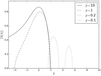
Figure 3 shows a graph of the instability growth rate|=(Λ)|versus the detuningδ for different

values ofρ¯. Forρ¯_{→ ∞}, it can be seen that Eq. (20) reduces to

Λ2(Λ−δ) + 1 = 0, (21)

which is the dispersion relation which would be obtained from a linear stability analysis of the classical FEL model, Eqs. (1)–(3) [11]. Similarly, the curve forρ¯= 10in Fig. 3 is almost identical to the classical FEL gain curve which would be obtained from Eq. (21), with the maximum growth rate at resonance (δ = 0). Asρ¯is decreased, the region of gain decreases in size and the value of detuning at which maximum gain occurs shifts to increasing values of δ such that δmax gain ≈ 1/2¯ρ, i.e., (γ0 −γr) ≈

~k/2mc.

−4 −2 0 2 4 6 8 10

δ

0.0 0.2 0.4 0.6 0.8

|ℑ

(λ

)|

¯ρ =10 ¯ρ =1 ¯ρ =0.2 ¯ρ =0.1

Fig. 3:Graph of growth rate against detuning,δ, for different values ofρ¯as calculated from Eq. (20)

4 One-dimensional quantum free-electron laser simulations

Using numerical simulations of the quantum FEL equations in either their position representation/Schrö-dinger form (Eqs. (12) and (13)) or their momentum representation (Eqs. (15) and (16)) allows investi-gation of the non-linear regime of the quantum FEL interaction. Here, results from simulations of the momentum representation equations are presented. In all cases shown, the initial condition corresponds to a monoenergetic/spatially uniform electron distribution such thatc0 = 1andck = 0∀k6= 0, and that

the radiation field amplitude is extremely small (_A¯_{= 10}−4_).

either the quantum, wave-function-based FEL model or the classical, particle FEL model whenρ¯ 1, which is consistent with this being the classical limit as discussed in Section 2. Figure 5 shows snapshots of the corresponding electron energy/momentum distribution for the case whereρ¯= 10andδ = 0. It can be seen that during the interaction, a large number of momentum states (∼ ρ¯) become populated, again consistent with the idea that this represents a classical regime of interaction.

0 5 10 15 20

¯z 10-8

10-7 10-6 10-5 10-4 10-3 10-2 10-1 100 101

|A

|

2

Fig. 4:Classical regime: evolution of radiation intensity,|A¯|2_{, whenρ¯= 10,δ= 0as calculated from Eqs. (15)}

and (16).

In contrast, Fig. 6 shows the evolution of the radiation field intensity as calculated from Eqs. (15) and (16) for a case whereρ¯= 0.1 andδ = 1/2¯ρ = 5, which should correspond to a quantum regime of interaction as discussed in Section 2. It can be seen that the field intensity evolves in a very different manner from that of the classical behaviour shown in Fig. 4 as a sequence of hyperbolic secant pulses. Figure 7 shows snapshots of the corresponding electron energy/momentum states. It can be seen that during the interaction, now only a maximum of two momentum states are populated at any stage of the interaction, the population cycling periodically between momentum statesn= 0andn=₋1, with one radiation pulse being emitted as the population cycles from state0_{→ −}1_→0. It can be shown that this evolution is well described by a model consisting of only two momentum states.

4.1 Including slippage

So far, it has been assumed that the relative slippage between the radiation field and the electrons due to their different velocities is negligible, so that the electron beam can be described in terms of a single ponderomotive potential with periodic boundary conditions such that every ponderomotive potential in the electron beam evolves identically. Here, the quantum FEL model is extended to include the effects of slippage, which allows the description of radiation pulse propagation and evolution during the quantum FEL interaction.

−40 −20 0 20 40 n

0.0 0.2 0.4 0.6 0.8 1.0

|cn

|

2

(a) ¯z =0

−40 −20 0 20 40

n 0.0

0.2 0.4 0.6 0.8 1.0

|cn

|

2

(b) ¯z =10

−40 −20 0 20 40

n 0.0

0.2 0.4 0.6 0.8 1.0

|cn

|

2

(c) ¯z =12

Fig. 5:Classical regime: snapshots of the electron momentum distribution,|cn|2, whenρ¯= 10,δ= 0as calculated

from Eqs. (15) and (16).

the (weak) initial bunching of electrons due to shot noise will vary randomly between different parts of the electron beam. It is important, therefore, to describe the effect of one part of the electron beam on the rest of the beam as mediated by the radiation field as it propagates forward through the electron beam.

To incorporate slippage into the models described so far, it is necessary to introduce an additional length scale which represents position in the electron bunch, i.e.,

z1=

z−vzt Lc

, (22)

where Lc = λ/4πρ is the ‘cooperation length’ [17] andvz is the mean axial velocity of the electron beam. .

Using this new independent variable, we can now define the radiation field amplitude_A¯_{and the} momentum state amplitudescnat each position along the electron bunch, i.e.,

¯

A(¯z)→A¯(¯z, z1),

cn(¯z)→cn(¯z, z1),

so that the quantum FEL equations in the momentum state representation, Eqs. (15) and (16), become the set of coupledpartialdifferential equations [18]

∂cn(¯z, z1)

∂z¯ = −i

n2

2¯ρcn−ρ¯ Acn¯ −1−A¯

∗_cn

+1, (23)

∂ ∂z¯+

∂ ∂z1

¯

A(¯z, z1) = ∞

X

n=−∞

cnc∗n−1+ iδA .¯ (24)

0 20 40 60 80 100 120 140 160 ¯z

0 2 4 6 8 10

|A

|

2

Fig. 6:Quantum regime: evolution of radiation intensity,|A¯_|2_{, whenρ¯= 0.1,δ= 5as calculated from Eqs. (15)}

and (16).

momentum amplitudes cn are distributed with random phases to simulate a stochastically fluctuating

bunching parameter along the electron bunch.

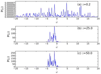
Snapshots of the spatio-temporal evolution of classical SASE radiation and its corresponding fre-quency spectrum are shown in Figs. 8 and 9, respectively. It can be seen that the evolution of the interaction results in a radiation field consisting of a sequence of random spikes of radiation, similar to what is produced in the classical model [11, 13]. Similarly, the corresponding frequency spectrum of classical SASE, shown in Fig. 9, is broad and chaotic. Note that the scaled frequency variable is defined asω¯ = (ω0−ωr)/ρωr, whereωr≈2cγr2kwis the resonant (angular) frequency of the radiation.

Corresponding graphs showing the spatio-temporal evolution of SASE radiation and its frequency spectrum in the quantum regime (ρ <¯ 1) are shown in Figs. 10 and 11, respectively. It can be seen that the evolution of the interaction in the quantum regime results in a radiation field which is amplified at a lower rate, but consists of a smoother, less spiky profile, with a frequency spectrum which evolves as series of discrete, narrow lines. Each discrete line is produced by transitions between successive momentum states, i.e.,n = 0 _{→ −}1 _{→ −}2, . . . . It can be shown [19] that the frequency separation

between these lines is∆ω = ~k2/γm, the recoil frequency associated with the emission of a photon

with momentum~kby a relativistic electron. The presence of these different discrete frequencies results

in a beating between these frequencies, which can be seen in the spatio-temporal evolution of the field for large values ofz¯(see, e.g., Fig. 10(b) and (c)). The existence of this beat note illustrates the phase coherence between the frequencies being generated.

−4 −2 0 2 4 n

0.0 0.2 0.4 0.6 0.8 1.0

|cn

|

2

(a) ¯z =0

−4 −2 0 2 4

n 0.0

0.2 0.4 0.6 0.8 1.0

|cn

|

2

(b) ¯z =37

−4 −2 0 2 4

n 0.0

0.2 0.4 0.6 0.8 1.0

|cn

|

2

(c) ¯z =80

Fig. 7:Quantum regime: snapshots of the electron momentum distribution|cn|2whenρ¯= 0.1,δ= 5as calculated

from Eqs. (15) and (16).

5 Realising the quantum free-electron laser regime

It was shown in Section 2 that the quantum FEL regime requires

¯

ρ= mcγ

~k ρ <1,

which can be rewritten as

γλ λc

ρ <1, (25)

whereλc = h/mc ≈ 2.4×10−12 m is the Compton wavelength. All current short-wavelength FELs operate in the classical regime; for example, the Linac Coherent Light Source (LCLS) has approximate parametersγ _≈3_×104_,ρ≈5×10−4_{, andλ≈1Å≈40λc, which from Eq. (25) givesρ¯≈600.}

Equation (25) shows that to attain the quantum regime whereρ <¯ 1without drastically reducing the FEL gain (∝ρ), then it is best to reduceλas far as possible (i.e., high photon momentum), but keep

γas small as possible. This would seem to be unfeasible for an FEL using a magnetostatic wiggler, such

0 10 20 30 40 50 60 70 z1

0.0000000 0.0000005 0.0000010 0.0000015 0.0000020 0.0000025 0.0000030

|A

|

2 (a) ¯z=0.2

0 10 20 30 40 50 60 70

z1

0 2 4 6 8

|A

|

2

(b) ¯z=25.0

0 10 20 30 40 50 60 70

z1

0 2 4 6 8 10

|A

|

2

(c) ¯z=50.0

Fig. 8: Snapshots of the spatio-temporal evolution of the classical regime of SASE (ρ¯ = 5) when the electron

bunch lengthLe= 20Lc.

−20 −15 −10 −5 0 5 10 15 20

¯ω 0.0000000.000001

0.000002 0.000003 0.0000040.000005 0.0000060.000007

P(

¯ω) (a) ¯z=0.2

−20 −15 −10 −5 0 5 10 15 20

¯ω 0

50 100 150

P(

¯ω)

(b) ¯z=25.0

−20 −15 −10 −5 0 5 10 15 20

¯ω 0

50 100 150 200 250

P(

¯ω)

(c) ¯z=50.0

0 20 40 60 80 100 120 140 160 z₁

0.0000000 0.0000005 0.0000010 0.0000015 0.0000020 0.0000025 0.0000030 0.0000035 0.0000040

|A

|

2 (a) ¯z=0.3

0 20 40 60 80 100 120 140 160

z1

01 2 3 4 5

|A

|

2

(b) ¯z=100.2

0 20 40 60 80 100 120 140 160

z1

01 2 3 4 5

|A

|

2

(c) ¯z=150.0

Fig. 10:Snapshots of the spatio-temporal evolution of the quantum regime of SASE (ρ¯= 0.2) when the electron

bunch lengthLe= 20Lc.

−20 −15 −10 −5 0 5 10 15 20

¯ω 0.0000000.000001

0.000002 0.000003 0.0000040.000005

P(

¯ω) (a) ¯z=0.3

−20 −15 −10 −5 0 5 10 15 20

¯ω 0

100 200 300 400

P(

¯ω)

(b) ¯z=100.2

−20 −15 −10 −5 0 5 10 15 20

¯ω 0

100 200 300 400 500

P(

¯ω)

(c) ¯z=150.0

6 Conclusions

In this article, the possibility of a quantum regime of FEL operation, the conditions under which quantum effects due to large photon recoil may be significant in the FEL interaction, and some of the features of the quantum FEL interaction have been discussed using a 1D model. Although the quantum regime of high-gain FEL operation has not yet been achieved, it appears that with current technology, realisation of the quantum FEL regime may be a possibility. Given that some spectral properties of the quantum FEL regime appear attractive relative to those of classical SASE FELs, for example improved temporal coher-ence, then the quantum FEL seems to have potential as a compact source of coherent, short-wavelength (X-ray/γ-ray) radiation.

Some recent and current work on quantum FELs which has not been covered in detail here is summarised below.

6.1 2D and 3D models

Although this article has concentrated on 1D models to illustrate concepts, both 2D and 3D quantum FEL simulations and models have been investigated [21,22]. Such studies are important to determine the conditions under which transverse inhomogeneities in and diffraction of the intense laser pulses used as electromagnetic wigglers will affect the quantum FEL gain process.

6.2 Spontaneous emission

It is well known that the stochastic kicks produced by spontaneously emitted photons can produce mo-mentum diffusion, which eventually quenches the classical FEL gain process at short wavelengths and provides an effective lower limit to the wavelength which can be produced by classical FEL operation ofλ_≈ 1Å. There has recently been some debate about the significance of the role which spontaneous emission will play in attempts to achieve the quantum regime of FEL operation [23, 24].

Finally, although the terminology of ‘quantum’ FEL has been used throughout this article, based on the conventional terminology used in the quantum optics literature, the models described here are more correctly described as ‘semiclassical’, as they use a quantum description of the medium (the elec-tron beam) but a classical description of the electromagnetic field. Fully quantum FEL models involving quantized radiation fields were developed long ago for the low-gain regime and used to investigate, for example, the photon statistics of the low-gain FEL interaction [3], and recent work has extended these models into the high-gain regime [16,25]. Such models offer the exciting prospect of opening up a whole range of new coherent, quantum, X-ray, andγ-ray phenomena, as has been done in the optical region of

the spectrum.

Acknowledgements

This article is dedicated to the memory of Rodolfo Bonifacio, who introduced me to the concept of the quantum free-electron laser. Many of the results described here arose from collaboration with Rodolfo and with Nicola Piovella.

References

[1] J. Madey,J. Appl. Phys.42(1971) 1906. https://doi.org/10.1063/1.1660466

[2] W. Becker and S. Zubairy,Phys. Rev. A25(1982) 2200. https://doi.org/10.1103/PhysRevA.25.2200 [3] W. Becker and J.K. McIver,Phys. Rev. A27(1983) 1030.

https://doi.org/10.1103/PhysRevA.27.1030

[4] J. Gea-Banacloche,Phys. Rev. A31(1985) 1607. https://doi.org/10.1103/PhysRevA.31.1607 [5] A. Friedman, A. Gover, G. Kurizki, S. Ruschin, and A. Yariv,Rev. Mod. Phys.60(1988) 471.

[6] P. Kling, E. Giese, R. Endrich, P. Preiss, R. Sauerbrey, and W.P. Schleich,New J. Phys.17(2015) 123019. https://doi.org/10.1088/1367-2630/17/12/123019

[7] R. Bonifacio, N. Piovella, and G.R.M. Robb,Nucl. Instrum. Methods Phys. Res. A543(2005) 645. https://doi.org/10.1016/j.nima.2005.01.324

[8] C.B. Schroeder, C. Pellegrini, and P. Chen,Phys. Rev. E64(2001) 056502. https://doi.org/10.1103/PhysRevE.64.056502

[9] G. Preparata,Phys. Rev. A38(1988) 233. https://doi.org/10.1103/PhysRevA.38.233 [10] B.W.J. McNeil and N.R. Thompson,Nat. Photonics4(2010) 814.

https://doi.org/10.1038/nphoton.2010.239

[11] R. Bonifacioet al.,Riv. Nuovo Cim.13(1990) 1. https://doi.org/10.1007/BF02770850

[12] J.B. Murphy and C. Pellegrini, inLaser Handbook, Vol. 6, Eds. W.B. Colsonet al.(North-Holland, Amsterdam, 1990), p. 9.

[13] E. Saldin, E.V. Schneidmiller, and M.V. Yurkov, The Physics of Free Electron Lasers(Springer, 2000).

[14] A. Tonomuraet al.,Am. J. Phys.57(1989) 117. https://doi.org/10.1119/1.16104 [15] M. Brown, J.R. Henderson, L.T. Campbell, and B.W.J. McNeil, in preparation.

[16] R. Bonifacio, N. Piovella, G.R.M. Robb, and A. Schiavi,Phys. Rev. Accel. Beams9(2006) 090701. https://doi.org/10.1103/PhysRevSTAB.9.090701

[17] R. Bonifacio, P. Pierini, and B.W.J. McNeil,Phys. Rev. A40(1989) 4467. https://doi.org/10.1103/PhysRevA.40.4467

[18] R. Bonifacio, N. Piovella, G.R.M. Robb, and M.M. Cola,Opt. Commun.252(2005) 381. https://doi.org/10.1016/j.optcom.2005.04.037

[19] R. Bonifacio, N. Piovella, M.M. Cola, and L. Volpe, Nucl. Instrum. Methods Phys. Res. A 577

(2007) 745. https://doi.org/10.1016/j.nima.2007.03.024

[20] R. Bonifacio, H. Fares, M. Ferrario, B.W.J. McNeil, and G.R.M. Robb,Opt. Commun.382(2017) 58. https://doi.org/10.1016/j.optcom.2016.07.007

[21] A. Schiavi, N. Piovella, G.R.M. Robb, and R. Bonifacio, Int. J. Mod. Phys. A 22 (2007) 4245. https://doi.org/10.1142/S0217751X07037792

[22] N. Piovella, M.M. Cola, L. Volpe, A. Schiavi, and R. Bonifacio,Phys. Rev. Lett.100(2008) 044801. https://doi.org/10.1103/PhysRevLett.100.044801

[23] G.R.M. Robb and R. Bonifacio,Phys. Plasmas19(2012) 073101. https://doi.org/10.1063/1.4729337

[24] G.R.M. Robb and R. Bonifacio,Phys. Plasmas20(2013) 124702. https://doi.org/10.1063/1.4838175