City, University of London Institutional Repository
Citation
:
Asimit, A.V., Badescu, A., Haberman, S. & Kim, E-S. (2016). Efficient risk
allocation within a non-life insurance group under Solvency II Regime. Insurance:
Mathematics and Economics, 66, pp. 69-76. doi: 10.1016/j.insmatheco.2015.10.008
This is the published version of the paper.
This version of the publication may differ from the final published
version.
Permanent repository link:
http://openaccess.city.ac.uk/13122/
Link to published version
:
http://dx.doi.org/10.1016/j.insmatheco.2015.10.008
Copyright and reuse:
City Research Online aims to make research
outputs of City, University of London available to a wider audience.
Copyright and Moral Rights remain with the author(s) and/or copyright
holders. URLs from City Research Online may be freely distributed and
linked to.
City Research Online: http://openaccess.city.ac.uk/ publications@city.ac.uk
Contents lists available atScienceDirect
Insurance: Mathematics and Economics
journal homepage:www.elsevier.com/locate/ime
Efficient risk allocation within a non-life insurance group under
Solvency II Regime
Alexandru V. Asimit
a,∗,1, Alexandru M. Badescu
b, Steven Haberman
a, Eun-Seok Kim
c aCass Business School, City University London, London EC1Y 8TZ, United KingdombDepartment of Mathematics and Statistics, University of Calgary, Calgary, Alberta T2N 1N4, Canada
cDepartment of International Management and Innovation, Middlesex University, London NW4 4BT, United Kingdom
a r t i c l e i n f o
Article history:
Received October 2015 Accepted 17 October 2015 Available online 31 October 2015
Keywords:
Best estimate Insurance group
Minimum Capital Requirement Risk margin
Solvency II
Solvency Capital Requirement
a b s t r a c t
Intra-group transfers are risk management tools that are usually widely used to optimise the risk position of an insurance group. In this paper, it is shown that premium and liability transfers could be optimally made in such a way as to reduce the amount of Technical Provisions and Minimum Capital Requirement for the entire insurance conglomerate. These levels of required capital represent the minimal amount that needs to be held by the insurance group without regulator intervention, according to the Solvency II regulation. We assume that only proportional risk transfers are feasible, since such transfers are not difficult to administer for a large scaled insurance group, as is always the case. In addition, any risk shifting should be made for commercial purposes in order to be considered acceptable by the local regulators that impose restrictions on how much the assets within an insurance group are fungible. Our numerical examples illustrate the efficiency of the optimal proportional risk transfers which can easily be implemented, in terms of computation, in any well-known solver even for an insurance conglomerate with many subsidiaries. We found that our proposed optimal proportional allocations are more beneficial for large insurance group, since the relative reduction in capital requirement tends to be small, whereas the gain in absolute terms is quite significant for large scaled insurance group.
©2015 The Authors. Published by Elsevier B.V. This is an open access article under the CC BY license (http://creativecommons.org/licenses/by/4.0/).
1. Introduction
Aninsurance group (IG)is composed of multiple legal entities, also known as insurance undertakings (IU’s), that may operate under different regulation regimes. Diversification across an IG represents a risk management tool, often used to reduce the risk exposures, and consequently the required level of capital within the organisation. The risk exposures of different entities will in general not be perfectly positively correlated, and thus somegroup level diversification is observed (seeKeller, 2007). On the other hand, assets and liabilities are not pooled across entities, since there are limits to the cross-subsidy (especially when conceptually different regulatory requirements are in place for various IU’s), as well as the capital fungibility, within the group. Nonetheless, the
∗Corresponding author. Tel.: +44 0 2070405282; fax: +44 0 2070408572.
E-mail addresses:asimit@city.ac.uk(A.V. Asimit),abadescu@math.ucalgary.ca
(A.M. Badescu),S.Haberman@city.ac.uk(S. Haberman),E.Kim@mdx.ac.uk
(E.-S. Kim).
1 The authors are listed in alphabetical order and contributed equally.
risk and capital requirements of individual entities can be reduced, through a web of capital and risk transfer arrangements across entities. This capital efficiency can be understood as a result of
down-streaming of diversification(seeKeller, 2007).
The complexity of group legal structures and intra-group risk transfers, with entities being potentially subject to different regulatory regimes, poses a major challenge for regulators, since it requires producing equivalence assessments between these regimes. For example, the EU and Swiss regulatory requirements are equivalent (see EIOPA, 2011), but no agreement has been achieved between these two regulatory bodies and the North American regulators. Therefore, it is not surprising that studying this problem has become a keen interest for practitioners and academics. The work ofFilipović and Kupper(2008) investigates optimal risk transfers in a framework where a finite set of risk transfer instruments is available and the capital requirements of individual entities are calculated via convex risk measures. The paper ofGatzert and Schmeiser(2011) studies the impact of group diversification on shareholder value, considering a variety of group structures and capital and risk transfer instruments, while also offering a thorough literature review of diversification in financial
http://dx.doi.org/10.1016/j.insmatheco.2015.10.008
70 A.V. Asimit et al. / Insurance: Mathematics and Economics 66 (2016) 69–76
conglomerates. Schlütter and Gründl (2012) assess the impact of group building on policyholder welfare. In their analysis, it is assumed that a particular type of rational risk transfer arrangement is enforced, while the group sets premium and equity targets in order to maximise shareholder value, allowing for the impact of entities’ default risk on insurance demand. A recent paper ofAsimit et al.(2013) investigates the optimal intra-group transfer in an IG consisting of two IU’s, where liabilities are assumed to be perfect positively associated.
An ambitious project, started more than a decade ago, has been initiated in order to harmonise the regulatory environment within the European Union (EU) insurance industry, which is known as Solvency II. This unified methodology applies to all insurance players that operate in the EU insurance market and its legal framework is specified inEuropean Commission(2009). The actual implementation of Solvency II is expected to be put in practice in several years, and in the meantime, various
Quantitative Impact Studies (QIS) have been performed. These QIS’s were meant to collect feedback from various insurance and reinsurance companies related to the constantly augmented Solvency II specifications. The most recent one, also known asQIS 5
(seeEuropean Commission, 2010), summarises the most probable recommendations that will later lead to the implementation of Solvency II.
In this paper, the optimal risk transfer within an EU non-life IG is considered. That is, all entities are located within EU or an equivalence assessment has been approved for the IU’s outside this economic region. In other words, the regulatory regime designed within the Solvency II equally applies to the entire IG. Since there are significant regulatory differences between life and non-life businesses, it is assumed that the IG is purely a non-life insurance one. Note that some non-life businesses, such as health insurance or workers’ compensation, are similar in nature to life insurance activities from the regulatory point of view, and therefore the capital requirements follow the life insurance evaluation. These hybrid businesses are excluded from our analysis, so that we could better understand the risk transfer effects within a pure non-life IG.
Optimising the risk intra-group transfers represents a practical problem that has not been discussed much in the framework of Solvency II, but there exists a rich literature on similar problems that exhibit a reduced level of complexity. One research stream is the optimal reinsurance contract problem that was first discussed byBorch(1960) andArrow(1963) who consider the objectives of minimising the variance of the insurer’s retained risk and maximising the expected utility of the insurer’s final wealth, respectively. Alternative decision criteria have been investigated by many researchers (see for example,Van Heerwaarden et al., 1989, Young, 1999, Verlaak and Beirlant, 2003, Kaluszka and Okolewski, 2008,Guerra and Centeno, 2008etc.). Decisions based on Value-at-risk (VaR) and Conditional Value-at-risk (CVaR) are considered byCai et al.(2008), Cheung(2010) andChi and Tan
(2011). A recent paper ofAsimit et al.(2015) identifies the optimal reinsurance contract by taking into account the Solvency II capital requirements. Note that the optimal reinsurance approach finds the ideal reinsurance contract between two insurance players, namely, insurer and reinsurer, where the risk shifting is usually initiated by the insurer in order to meet the solvency targets. A more cooperative approach is the so-called optimal risk allocation problem that has a long history. Under this setting, the players have their own targets and try to efficiently share their risks in a way that is mutual beneficiary to all risk holders, i.e. finding the Pareto optimal risk transfers. The vast literature on this topic includes
Landsberger and Meilljson(1994),Ludkovski and Young(2009),
Kiesel and Rüschendorf (2009, 2010),Carlier et al.(2012) etc. An excellent review on this topic has appeared inRüschendorf(2013).
In summary, the main aim of this paper is to identify the optimal risk allocation within a non-life IG such that the total IG minimum level of capital is reduced as much as possible. The paper is organised as follows: Section2provides the necessary background on Solvency II and describes our setting, while Section3contains a case study that numerically illustrates our previous findings; the main conclusions of the paper are summarised in Section4.
2. Capital requirements model
The main purpose of the paper is to explain how an IG may ef-ficiently share their various risk portfolios in order to reduce the capital requirements. The chosen regulatory environment is the Solvency II Regime that applies to a large economic area and there-fore, it is likely to consider the problem of capital efficiency of an in-surance conglomerate. In Section3, we will consider the economic value captured by the IG when implementing such risk manage-ment tools. In order to define the ultimate objective function that we need to optimise, we need to describe the capital requirements model used in this paper, which is a replication of the current Sol-vency II recommendations, as defined in previous QIS’s such as QIS4 (seeEuropean Commission, 2008) and QIS5 (for example, see
European Commission, 2010). Recall that QIS5 provides a signif-icant augmentation to QIS4, not only on the parameter values of the considered proxy models, but there are conceptual differences in implementing the Solvency II recommendations.
We assume that we have an IG consisting ofnIU’s that operates under the Solvency II Regime and each IU holdsm lines of business (LOB’s). There are twelve LOB’s recognised within Solvency II, which are life insurance, while three other LOB’s are non-life insurance, but the corresponding capital requirements follow the life insurance evaluation. The capital requirements are set up for a finite time horizon, which is one year for Solvency II. The EU regulatory regime requires capital to be put aside in order to cover thetechnical provisions (TP)and additional capital. The TP’s are evaluated per LOB, and each of them consists ofbest estimate (BE)of the liabilities and itsrisk margin (RM)(see for example,
CEIOPS, 2010). The additional capital is defined asMinimum Capital Requirement (MCR)andSolvency Capital Requirement (SCR). MCR is viewed as the lower bound of the SCR, and immediate regulatory intervention is in force once an IU holds capital at levels lower than its MCR. The SCR calculations within an IG are very complex, and lead to individual calculations for stand-alone IU’s and IG calculations by taking into account the consolidated balance sheet (where the risk transfers cannot be used as a risk management tool), but each IU should calculate their very own SCR, called the individual SCR. The MCR calculations are much simpler, and at a group level, the total MCR equals to the sum of all MCR’s. Besides the fact that MCR and SCR are calculated in a different manner, the required own funds to cover these levels of capital should satisfy certain requirements. As expected, the requirements are more stringent for the assets that are allowed to reach the MCR level than the SCR level.
and future liabilities in the same proportion. That is, letxijkbe the
proportion of business volume, pertaining to thekth LOB, received by theith IU from thejth IU. The case in whichi
=
jshould be understood as the remaining business held by thejth IU. Clearly,n
i=1
xijk
=
1,
xijk≥
0,
for all 1≤
i≤
n,
1≤
k≤
m.
In addition, it is assumed that all transfers are made at the same time.
We now explain the Solvency II terminology for calculating the three major capital requirements components: BE, RM and MCR. The first component is relatively simple, and each IU should report the BE’s gross and net of ‘‘reinsurance’’. Since the BE represents the expected value of future liabilities, the IG’s total amount of BE’s remains the same on both calculation methods and more importantly, it is not sensitive to any kind of risk shifting. Consequently, our model may discard the BE contributions to the TP.
The most granular methodology is related to the RM calculation. Note that the RM’s are evaluated without allowing any diversifi-cation between different LOB’s of any particular IU, and therefore calculations are extremely simplified. In addition, RM calculations take into account only four sources of risk:underwriting (UwR), un-avoidable market (UMR), counterparty default (CDR) and operational (OpR). The calculations for the UwR risk include thepremium (PR) and reserve (RR)risks.
LetRMikbe the corresponding RM for thekth LOB of theith IU.
Recall that RM’s are calculated per LOB, and the total RM for a given IU is given by summing the individual RM’s (seeCEIOPS,2009,
2010). Therefore, the IG’s total RM capital requirements becomes:
RMIG
:=
n
i=1 m
k=1
RMik
.
(2.1)Note that the calculations of OpR for a non-life IG is simplified to
SCROpRik
:=
0.
03P−gross1,ik+
max
0.
03P−gross1,ik−
1.
1P−gross2,ik,
0
,
whereP−gross1,ikandP−gross2,ikare gross (of reinsurance and intra-group transfer) earned premium received by theith IU for thekth LOB during the last year and year before last year, respectively. Note that the earned premiums are calculated in this paper via the accounting method due to its simplicity, especially when defining the net earned premiums needed for the PR calculations. Clearly, the OpR contribution to the capital requirements is evaluated gross of any risk transfer, and therefore, our optimisation problem may neglect this capital requirement component, which is not the case for the remaining four risks. Thus, after removing the OpR, the mathematical formulation for eachRMikfollows theCost-of-Capital
approach and is given by:
λ
SCRtfik+
1+
r2
Durmodik
−
nik
Durmodik
−
nik+
1
1rnikBE
net ik
+
SCRCDRik
,
(2.2)where
(i)
λ
=
CoC/(
1+
r)
is the adjustment coefficient with CoCandrbeing the Cost-of-Capital rate and annual risk-free rate, respectively;
(ii)SCRtfikrepresents the current SCR for thekth LOB of theith IU, excluding market risk and default for financial derivatives; (iii) Durmod
ik defines the modified duration ofBEnetik ;
(iv)nik is the longest duration of available risk-free financial
instruments to cover the liabilities corresponding to thekth LOB of theith IU;
(v) 1rnikrepresents the absolute decrease of the risk-free interest
for maturity nik under a downward stress scenario of the
interest rate risk sub-module;
(vi) BEnetik defines the net BE provisions for the claims outstanding in thekth LOB of theith IU;
(vii)SCRCDRik is the current capital charge for the default risk within thekth LOB of all transfers made by theith IU.
It is common sense to have thatDurmodik
=
Durmodk for all 1≤
k≤
n, i.e. the modified duration depends only on the nature of the busi-ness rather than being geographically specific for similar insurance risks. Now, several recommendations have been made for calculat-ing the previously-mentioned quantities. The first simplification is for computingSCRtfik, where only the PR and RR risks are taken into account. These risks are assumed to be LogNormal distributed with meansPiknetandBEnetik , and coefficients of variationσ
ikPRandσ
ikRR, where(i)
σ
PRik and
σ
ikRRrepresent the standard deviation for PR and RR,respectively, corresponding to thekth LOB of the ith IU, as defined by the Solvency II Standard Formula;
(ii) Pnet
ik is the net (of reinsurance and intra-group transfer) earned
premium in thekth LOB of theith IU during the forthcoming year.
Note that for a LogNormal random variable,Z, with mean
µ
and coefficient of variationσ
, we haveVaRp
(
Z)
−
E(
Z)
=
µ
exp
{
Φ−1(
p)
√
1
+
σ
2}
√
1
+
σ
2−
1
,
whereVaRp
(
Z)
andΦ−1(
p)
are thep% percentile of the distributionfunction ofZand standard normal, respectively. Denote
g
(
t)
:=
exp
Φ−1
(
p)
log
1
+
t2
√
1
+
t2−
1.
(2.3)According to QIS5,p
=
99.
5% andSCRtfik
:=
g
σPR
ik
Piknet
2
+
g
σRR
ik
BEnetik
2
+2αg
σPR
ik
g
σRR
ik
PiknetBEnetik ,
(2.4) where
α
(usually is 0.5) represents the correlation coefficient between PR and RR, as defined by the Standard Formula. Market wide estimates forσ
are shown to be between 5% and 22%, and therefore, a reasonable approximation, g(σ )
≈
3σ
, has been proposed in QIS4 and QIS5, but we prefer to work with the formulation displayed in Eq.(2.4)in order to achieve a more accurate evaluation of the capital requirements. The general rule in Solvency II for the proportional evaluation of the risk leads toPiknet
:=
n
j=1
xijkPjkgross and BE
net
ik
:=
n
j=1
xijkBEgrossjk
,
(2.5)wherePjkgrossis the gross earned premium in thekth LOB of thejth IU during the forthcoming year before making any transfer. Note that diversification among LOB’s or IU’s is not allowed in the calculation of the RM’s. In addition,
σ
PRik
=
σ
kPRandσ
ikRR=
σ
kRRare assumed tobe constant among all IU, and their tentative values are tabulated in Section 2 ofEuropean Commission(2010), but one should keep in mind that the calibration process is still under development, which is one of the scopes of each QIS.
The second term from relation(2.2)represents the contribution of the UMR, which is a simplification recommended in Section 2
72 A.V. Asimit et al. / Insurance: Mathematics and Economics 66 (2016) 69–76
guidance to calculating the regulatory CDR capital, which is defined for two classes of exposures. According to the Solvency II terminology, the intra-group transfers belong to the class of type 1 exposures. In addition, common practice suggests the same
probability of default (PD)for all IU’s, which is usually estimated from external ratings or based on the IGsolvency ratio (SR)(i.e. the ratio between IG total own funds and capital requirements). Moreover, for regulation purposes, the IG needs to evaluate theLoss Given Default (LGD)for each subsidiary, where the LGD represents the loss of basic own funds which a subsidiary would incur if the another subsidiary or subsidiaries default. The LGD is amended by 1
−
RecR, whereRecRrepresents therecovery rateof the IU, and the European Commission recommendations include that the RecR’s should be estimated based on the specific risk profile of each subsidiary. Thus, without loss of generality, it is further assumed that all LOB’s of a single IU have the same RecR, but different values may arise among distinct IU’s. Whenever robust estimation of the RecR is not possible, the recommendation is to use the 50% benchmark value. The capital requirements for type 1 exposures is recommended to beSCRCDRik
:=
3
Vik,
Vik
≤
5%
j̸=i LGDik
min
j̸=i
LGDjk
,
5
Vik
,
Vik
>
5%
j̸=i LGDik
,
whereVikandLGDikrepresent the variance of the loss distribution
of the type 1 exposures and LGD in theith LOB of theith IU. This formulation may lead to arbitrage opportunities, which can be removed by considering the following reformulation:
SCRCDRik
:=
min
j̸=i LGDjk
,
l
Vik
,
(2.6)wherelis a constant.
TheLGDikresults from the potential loss in own funds due to PR
and RR risks, and one needs to take advantage of the LogNormal assumption. It is not difficult to find that a LogNormal random variable,Z, with mean
µ
and coefficient of variationσ
, satisfiesE
Z
−
VaRp(
Z)
|
Z>
VaRp(
Z)
=
µ
1
−
pΦ
log
1+
σ
2
−
Φ−1(
p)
−
VaRp(
Z),
whereΦis the distribution function of a standard normal random variable. Denote
h
(
t)
:=
Φ
log
1+
t2
−
Φ−1(
p)
1
−
p−
g(
t)
−
1,
(2.7)where function g is defined in Eq. (2.3). Since the capital requirements are set atVaR99.5%level, then we have
LGDik:=(1−RecRi) ×
hσPR ik Pnet ik 2 +
hσRR ik
BEnetik
2
+2αhσPR ik
hσRR
ik Pnet ik BE net ik , (2.8) where once again
α
=
0.
5 andp=
99.
5%. As anticipated,RecRirepresent the recovery rate corresponding to theith IU.
The Vik takes into account the default within the kth LOB
of all other IU’s, except for the ith IU. Due to the dependence between these default events, the evaluation of the varianceVik
should include the concomitant default events, which makes the calculations quite laborious if all concomitant default events are included. Since the PD for multiple IU at the same time decreases
significantly once the number of insolvent IU’s increases, it is further assumed that no more than two concomitant default events may occur at the same time. Note that in these situations, we may aggregate the defaulted amounts if the assets are non-fungible, which is normally the case, unless a legally binded contract is in force (for further details, seeKeller, 2007). Therefore,Lik, the
random loss in own funds for thekth LOB of theith IU, is given by
Lik
:=
LGDjk
,
if only thejth IU defaults,
j̸=
i LGDj1k+
LGDj2k,
if only thej1thandj2th IU’s default
,
j1<
j2,
j1,
j2̸=
i.
The PD’s do not vary among different IU’s, and for this reason, we may denotep1 and p2 to be the PD of a single default only
and concomitant default, respectively. Within QIS5, there are recommended values for the PD (single or concomitant) of an IU and are equal top1
+
p2(
n−
1)
. It is expected that the concomitantevents are stochastically positively dependent, which implies that
PD2
≤
p2. Thus, one may require to havePD2≤
p2≤
PD/(
n−
1)
.Simple calculations show that
E
Lik
=
p1
j̸=i
LGDjk
+
p2
j1<j2,j1,j2̸=i
LGDj1k
+
LGDj2k
=
PD
j̸=i LGDjk
and
E
L2ik
=
p1
j̸=i
LGD2jk
+
p2
j1<j2,j1,j2̸=i
LGDj1k
+
LGDj2k
2=
PD
j̸=i
LGD2jk
+
2p2
j1<j2,j1,j2̸=i
LGDj1kLGDj2k
=
p2
j̸=i LGDjk
2+
(
PD−
p2)
j̸=i LGD2jk
.
Thus, the latter equations and(2.6)yield that
SCRCDR ik :=min j̸=i LGDjk,l
p2−PD2 j̸=i LGDjk 2
+(PD−p2)
j̸=i LGD2jk
.
It is worth mentioning that an IG that is financially stable may simplify the CDR calculations as follows:
SCRCDRik
=
l
p2−
PD2
j̸=i LGDjk
2+
(
PD−
p2)
j̸=i LGD2jk
.
(2.9) Note that the positiveness ofPD
−
p2implies that the above is trueas long asl2PD2
−
l2PD+
1≥
0 or equivalently ifPD(
1−
PD)
≤
1/
l2. Ifl=
3 then the latter is satisfied wheneverPD≤
12.
73%, which is true, according to the QIS 5 recommendations (seeEuropean Commission, 2010), for an IG with a B rating or higher or any unrated IG (i.e. any possible SR satisfies our sufficient condition whenever the IG is unrated). Similarly, ifl=
5 then we should havePD≤
4.
17%, which is true for an IG with a BB rating or higher or a SR larger than 80% for an unrated IG. Consequently, the simplified formula from(2.9)can be utilised for an IG with a reasonable financial stability.Finally, we need to define the MCR contribution to our objective function, i.e. the IG’s total MCR,MCRIG. As anticipated, the latter
quantity is obtained by aggregating all MCR’s:
MCRIG
:=
n
i=1
whereMCRi represents the individual MCR corresponding to the ith IU. Each MCR includes the linear MCR for pure non-life business and for non-life business similar to life business. Since we deal with a pure non-life IG, the second component is not present in this model. Therefore,
MCRi
:=
m
k=1
max
α
kBEnetik, β
kP−net1,ik
,
(2.11)where
α
kandβ
kare some constants, whileP−net1,ikrepresents thenet (of reinsurance and intra-group transfer) written premiums within the kth LOB of the ith IU (for details, see Section 4 of
European Commission, 2010). It is worth mentioning that each
MCR is assumed to lie between 20% and 50% of the corresponding individual SCR, which has been confirmed by empirical evidence accumulated in the results of the QIS5 among the EU IG’s, when the Standard formula of Solvency II was implemented. Finally, by putting together relations(2.5),(2.10)and(2.11), one may find that the total RM is given by:
MCRIG
=
n
i=1 m
k=1
max
α
k n
j=1 xijkBE
gross
jk
, β
kP−net1,ik
.
(2.12)3. Numerical examples
In this section, we discuss the implementation of our optimi-sation problem and provide a numerical example to illustrate the effect of the proposed risk transfer methodology. First, we need to rewrite the optimisation problem such that the new formula-tion is implementable in any well-known optimisaformula-tion software. For the sake of simplicity, the following notations are made for all 1
≤
i≤
nand 1≤
k≤
m:aik
=
Pikgross,
bik=
BEgrossik,
cik
=
λ
1
+
r2
dk
−
nik
dk
−
nik+
1
1rnik
,
dk=
Durmodk,
e1
=
l2
p2
−
PD2
,
e2=
l2
PD
−
p2
,
Pik=
β
kP−net1,ik,
sk=
λ
g
σ
PRk
,
tk=
λ
g
σ
RRk
,
uk
=
λ
h
σ
PR k
,
v
k=
λ
h
σ
RRk
,
where the function g and h are defined in (2.3)and (2.7). In addition, definef
(
x,
y)
:=
x2+
y2+
xyandFik
(
x)
:=
(
1−
RecRi)
f
uk n
l=1
xilkalk
, v
k n
l=1 xilkblk
.
Clearly, a combination of(2.1),(2.2),(2.4),(2.5),(2.8),(2.9)and
(2.12)yield that our optimisation problem is given by: min
x∈ℜn×n×m
m
k=1 n
i=1
f
sk n
j=1
xijkajk
,
tk n
j=1 xijkbjk
+
cik n
j=1
xijkbjk
+
max
α
k n
j=1
xijkbjk
,
Pik
+
min
e1
j̸=i Fjk
(
x)
2+
e2
j̸=i
Fjk2
(
x),
j̸=i Fjk
(
x)
s.t. n
j=1
xijk
=
1,
xijk≥
0 for all 1≤
i,
j≤
nand 1≤
k≤
m.
[image:6.595.317.562.310.440.2](3.1) The above unconstrained optimisation problem is economically sound if each IU has sufficient assets to cover its TP and MCR after
Table 3.1
The values ofαk,βk,σkPR,σkRRanddk, where the first four quantities are chosen as
defined in QIS5.
k LOBk αk βk σkPR σkRR dk
1 Motor, third-party liability 12% 13% 10% 9.5% 2.3
2 Motor, other classes 13% 9% 7% 10% 1.86
3 Marine, aviation, transport 18% 22% 17% 14% 2.03
4 Fire and other property damage 14% 13% 10% 11% 1.56
5 Third-party liability 14% 20% 15% 11% 3.79
6 Credit and suretyship 25% 28% 21.5% 19% 2.72
7 Legal expenses 12% 9% 6.5% 9% 1.45
8 Assistance 14% 7% 5% 11% 1.75
9 Miscellaneous 20% 17% 13% 15% 3.03
the transfers have been made. Recall that for the sake of exposition, our model excludes the BE’s and OpR contribution to the RM, since both are gross of any risk transfers. Therefore, let us denote byAi
the available assets held (before the risk transfers take place) by the
ith IU, where the BE’s and OpR contribution to the RM calculations are removed. A set of transfers is feasible if each IU holds sufficient own funds to cover the new portfolio of liabilities. Therefore, the optimisation problem from(3.1)should be augmented by adding the following set of inequality constraints:
m
k=1
f
sk n
j=1
xijkajk
,
tk n
j=1 xijkbjk
+
cik n
j=1
xijkbjk
+
max
α
k n
j=1
xijkbjk
,
Pik
+
min
e1
j̸=i Fjk
(
x)
2+
e2
j̸=i
Fjk2
(
x),
j̸=i Fjk
(
x)
≤
Ai+
j̸=i m
k=1
xijkajk
−
xjikaik
,
for all 1≤
i≤
n.
(3.2)A detailed discussion on the convexity of the above objective function and constraints is presented in theAppendix, where we propose a reformulation of our optimisation problem as a Mixed Integer Nonlinear Programming (MINLP) problem. For numerical purposes, the optimal problem displayed in Eq. (A.2) from
Appendixis implemented using the General Algebraic Modeling
System (GAMS), a high performing solver which accommodates our setting very well.Table 3.1provides the values for
α
’s,β
’s andσ
’s parameters as suggested in QIS5 (for details, see Sections 2 and 4 ofEuropean Commission, 2010). In addition, realistic values fordkare also provided inTable 3.1, which have been chosen after
consulting many UK based non-life insurance companies. Among the twelve pure non-life LOB’s, we chose only nine, i.e.m
=
9, since the other three refer to reinsurance, which without loss of generality are excluded from our model since our aim is to allocate efficiently the IG’s assets and liabilities without reducing its overall business volume.It is also assumed that the gross earned premiums for the forthcoming year and net written premiums in the previous year are the same for all LOB’s and IU’s, i.e.Pnet
−1,ik
=
aik. In addition,the annual risk-free interest is 4%. As it can be seen inTable 3.1, the possible maximal maturity for the risk-free interest is three years. The values for1rnare suggested in Section 2 ofEuropean
Commission (2010), where the downward stress scenarios are
defined to a reduction in the annual risk-free interest of 75%, 65% and 56% for a maturity of one, two and three years, respectively. Thus,1rnequals to 3%, 2
.
6% and 2.
24% for a maturity of one, two74 A.V. Asimit et al. / Insurance: Mathematics and Economics 66 (2016) 69–76
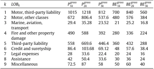
Table 3.2
Sensible values ofPgross’s andBEgross’s for all three IU’s (figures are in millions).
k LOBk P1grossk P gross 2k P
gross 3k BE
gross 1k BE
gross 2k BE
gross 3k
1 Motor, third-party liability 1015 1218 812 700 840 560
2 Motor, other classes 672 806.4 537.6 480 576 384
3 Marine, aviation, transport
29.4 35.28 23.52 21 25.2 16.8
4 Fire and other property damage
490 588 392 280 336 224
5 Third-party liability 558 669.6 446.4 360 432 288
6 Credit and suretyship 86.4 103.68 69.12 48 57.6 38.4
7 Legal expenses 28 33.6 22.4 20 24 16
8 Assistance 42 50.4 33.6 30 36 24
9 Miscellaneous 72.5 87 58 50 60 40
Our numerical examples assume an IG with three IU’s, i.e.n
=
3, and we report inTable 3.2the best estimate of liabilities and earned premiums for each IU and LOB. The values for the first IU are chosen to be similar to those of Aviva Insurance Limited which can be found on their publicly available statement of solvency. For the second IU, the best estimates of liabilities are taken to be 20% higher, while for the third IU they are 20% lower; the corresponding security loadings necessary for premium calculations are kept constant for all LOB’s. Note that the values forcikare computed via
the formula from the beginning of this section by usingnik
= ⌊
dik⌋
,for all 1
≤
i≤
nand 1≤
k≤
m. We consider a default probability of 0.05% and lete1=
0.
000624375 ande2=
0.
009371875. Thetotal assets held by each IU is our last input and these values are: 1406.020, 1687.224 and 1124.816 (figures are in millions).
The optimisation problem (A.2) is run under two different scenarios depending on the values of the recovery rates. In the first case, we assume that all IU’s have the same recovery rate of 0.5, while in the second case we assume that RecR1
=
0.
5, RecR2=
0.
6 andRecR3=
0.
4. The optimal solutions are displayedin Tables 3.3 and 3.4. It has been implicitly assumed that all IU’s are already operating, so that the costs of opening a new business unit are not included in this analysis. Otherwise, obtaining geographic diversification by expanding the IG would need to take into account the emerging friction costs.
We notice that the optimal risk transfer solutions are very sensitive to the recovery rates of each IU. Although some of
the weights remain the same (see for example the risk transfer performed by the first IU for the first five LOB and for the last one), most of them change. More importantly, we can analyse the effect of these recovery rates by computing the gain from transferring the risk versus the no-transfer case. We can define this gain as the relative difference between the objective function evaluated based on the optimal solutions and the trivial solution (i.e.xijk
=
1, foranyi
=
j, andxijk=
0 for anyi̸=
j). Under the same recoveryrate scenario, we notice that this difference is negligible, of around 5
·
10−6%. However, this is no longer the case for the secondscenario where the relative difference is around 0
.
01%. Thus, we have constructed a numerical example in which we showed that the recovery rate is an important factor in choosing the optimal risk transfer between insurance undertakings, and the gain by taking such a strategy can be quite significant.4. Conclusions
In this paper, we have translated the capital requirements for a non-life insurance company operating under Solvency II into math-ematical form and then considered the problem of determining the efficient allocation of risk across LOB’s by following the most re-cent Solvency II recommendations summarised in QIS5. The pro-portional allocation represented the set of feasible risk transfers, since the administration costs within the IG are very low and more importantly, due to the fact that proportional allocations are ac-ceptable to local regulators. One may consider non-proportional allocations that have a commercial purpose in order to be feasible from the local regulators’ point of view, but sharing the premiums in a ‘‘fair’’ manner is quite problematic and moreover, the adminis-tration costs may escalate. Therefore, non-proportional allocations may not be profitable to the IG and future investigations may clar-ify how beneficial it would be to an IG to allocate the risks in this fashion.
[image:7.595.119.469.523.619.2]The model contains a large number of parameters representing the features of each IU and LOB. We have not shown the sensitivity of the results to changes in all of the parameters since the optimal allocation is not sensitive to many of the underlying parameters. However, our work to date suggests that a key parameter is the recovery rate assumed for each IU. For numerical purposes, we
Table 3.3
Optimal intra-group transferring proportions for the problem defined in(A.2)with three IU with the same recovery rates.
k LOBk x∗11k x ∗ 21k x
∗ 31k x
∗ 12k x
∗ 22k x
∗ 32k x
∗ 13k x
∗ 23k x
∗ 33k
1 Motor, third-party liability 0.10 0.90 0.00 1.00 0.00 0.00 0.33 0.33 0.33
2 Motor, other classes 0.00 0.46 0.54 0.81 0.00 0.19 0.00 1.00 0.00
3 Marine, aviation, transport 1.00 0.00 0.00 0.59 0.00 0.41 0.00 1.00 0.00
4 Fire and other property damage 1.00 0.00 0.00 0.52 0.00 0.48 0.00 1.00 0.00
5 Third-party liability 1.00 0.00 0.00 0.66 0.00 0.34 0.54 0.46 0.00
6 Credit and suretyship 0.94 0.00 0.06 0.03 0.00 0.97 0.00 0.52 0.48
7 Legal expenses 0.16 0.68 0.16 0.34 0.38 0.28 0.57 0.00 0.43
8 Assistance 1.00 0.00 0.00 0.00 0.28 0.72 0.00 1.00 0.00
[image:7.595.120.471.657.753.2]9 Miscellaneous 0.59 0.41 0.00 0.00 0.18 0.82 0.81 0.19 0.00
Table 3.4
Optimal intra-group transferring proportions for the problem defined in(A.2)with three IU with different recovery rates.
k LOBk x∗11k x ∗ 21k x
∗ 31k x
∗ 12k x
∗ 22k x
∗ 32k x
∗ 13k x
∗ 23k x
∗ 33k
1 Motor, third-party liability 0.64 0.17 0.19 0.77 0.00 0.23 0.00 0.00 1.00
2 Motor, other classes 0.00 0.36 0.64 0.81 0.00 0.19 0.00 1.00 0.00
3 Marine, aviation, transport 1.00 0.00 0.00 0.19 0.00 0.81 0.50 0.00 0.50
4 Fire and other property damage 1.00 0.00 0.00 0.22 0.00 0.78 0.45 0.09 0.45
5 Third-party liability 0.43 0.00 0.57 0.00 0.00 1.00 1.00 0.00 0.00
6 Credit and suretyship 0.94 0.00 0.06 0.37 0.00 0.63 0.00 0.00 1.00
7 Legal expenses 0.00 0.74 0.26 0.35 0.30 0.35 0.79 0.00 0.21
8 Assistance 0.70 0.04 0.26 0.00 0.00 1.00 0.00 1.00 0.00
have illustrated the model with a simple, but realistic case study. This demonstrates that the optimisation routine does not lead to a trivial solution, so weightsxijkare not equal to one. In the
case study, we found that the optimal (total) capital requirements (included in our objective function) does not change much in relative terms (around 0.01%), but in absolute terms, the reduction in the level of required capital could be significant for a large IG.
Acknowledgements
The authors would like to thank an anonymous referee for help-ing in improvhelp-ing the paper. The authors would also like to acknowl-edge the practitioner advice received from Dr. Peter England on the choice of parameter values for the model. The second author would like to thank the Natural Sciences and Engineering Research Coun-cil of Canada (NSERC) for its continuing support.
Appendix
First, we note that the function f
(
·
)
from(3.1) is a convex function onℜ
2, and thus, any composition with an affine mappingforf
(
·
)
is a convex function as well, and in turn, the first term of the objective function from Eq.(3.1)is a convex function. In addition, the third term of the objective function from Eq.(3.1)is a convex function as well. Therefore, we deal with a convex optimisation problem as long as the simplified formulae from(2.9)holds. In other words, for an IG with a ‘‘good’’ credit risk, we can rewrite the optimisation problem as follows:min
(x,u)∈ℜn×n×m×ℜn×m
m
k=1 n
i=1
f
sk n
j=1
xijkajk
,
tk n
j=1 xijkbjk
+
cik n
j=1
xijkbjk
+
uik+
e1
j̸=i Fjk
(
x)
2+
e2
j̸=i F2
jk
(
x)
s.t. n
j=1
xijk
=
1,
xijk≥
0for all 1
≤
i,
j≤
nand 1≤
k≤
m,
α
k n
j=1
xijkbjk
≤
uik,
Pik≤
uikfor all 1
≤
i≤
nand 1≤
k≤
m,
m
k=1
f
sk n
j=1
xijkajk
,
tk n
j=1 xijkbjk
+
cik n
j=1
xijkbjk
+
uik+
e1
j̸=i Fjk
(
x)
2+
e2
j̸=i F2
jk
(
x)
≤
Ai+
j̸=i m
k=1
xijkajk
−
xjikaik
,
for all 1≤
i≤
n.
(A.1)
Here, the slack variablesuikare introduced in order to produce an
implementable (differentiable and convex) optimisation problem. Note that if relation(2.9)does not hold, there is an alternative solution to our optimisation problem, namely a Mixed Integer Nonlinear Programming (MINLP) formulation for(3.1)with the restriction from(3.2). Therefore,(A.1)is now replaced by a MINLP reformulation due to the min’s terms in both the objective function and constraint. In order to remove this term we need to add the binary variablesyik
∈
A= {
0,
1}
and the slack variablesv
ik. LetMbe a sufficiently large number. Then, the MINLP reformulation can be argued as inAsimit et al.(2015) and is given by:
min
(x,y,u,v)∈ℜn×n×m×An×m×ℜn×m×ℜn×m
m
k=1 n
i=1
f
sk n
j=1 xijkajk
,
tk n
j=1 xijkbjk
+
cik n
j=1
xijkbjk
+
uik+
v
ik
s.t.
n
j=1
xijk
=
1,
xijk≥
0 for all 1≤
i,
j≤
nand 1≤
k≤
m,
α
k n
j=1
xijkbjk
≤
uik,
Pik≤
uik,
j̸=i
Fjk
(
x)
+
M(
yik−
1)
≤
v
ik,
v
ik≤
j̸=i Fjk
(
x),
v
ik≤
e1
j̸=i Fjk
(
x)
2+
e2
j̸=i F2
jk
(
x)
and
e1
j̸=i Fjk
(
x)
2+
e2
j̸=i F2
jk
(
x)
−
Myik≤
v
ik,
for all 1
≤
i≤
nand 1≤
k≤
m,
m
k=1
f
sk n
j=1
xijkajk
,
tk n
j=1 xijkbjk
+
cik n
j=1
xijkbjk
+
uik+
v
ik
≤
Ai+
j̸=i m
k=1
xijkajk
−
xjikaik
,
for all 1≤
i≤
n.
(A.2)
Note that there are nonlinearities in both the objective function and constraints in the(A.2), and thus, it is possible to not be able to find an optimal solution in a reasonable time for large dimensional problem. This is not the case for practical problems, where it is not expected to have more than let say 10 IU’s, i.e.n
≤
10. Since we know thatk≤
13, then even for large IG with 10 subsidiaries, the dimension of our problem would be 102×
13+
3×
10×
13=
1690,which can be efficiently accommodated by a commercial solver such as GAMS. For example, in our case the optimal solution is found in less than a second using an Intel Core i7-2600, 3.40 GHz processor and 8 GB RAM.
References
Arrow, K.J.,1963. Uncertainty and the welfare economics of medical care. Amer. Econ. Rev. 53 (5), 941–973.
Asimit, V., Badescu, A., Tsanakas, A.,2013. Optimal risk transfers in insurance groups. Eur. Actuar. J. 3 (1), 159–190.
Asimit, A.V., Chi, Y., Hu, J.,2015. Optimal non-life reinsurance under solvency II regime. Insurance Math. Econom. 65, 227–237.
Borch, K., 1960. An attempt to determine the optimum amount of stop loss reinsurance. Transactions of the 16th International Congress of Actuaries, vol. I, pp. 597–610.
Cai, J., Tan, K.S., Weng, C., Zhang, Y.,2008. Optimal reinsurance under VaR and CTE risk measures. Insurance Math. Econom. 43 (1), 185–196.
Carlier, G., Dana, R.-A., Galichon, A.,2012. Pareto efficiency for the concave order and multivariate comonotonicity. J. Econom. Theory 147 (1), 207–229.
CEIOPS, 2009. Draft CEIOPS’s advice for LEVEL 2 implementing
mea-sures on solvency II: Article 85(d), Calculation of the Risk Margin, Consultation Paper 42, CEIOPS-CP-42/09. Available at: https://eiopa. europa.eu/fileadmin/tx_dam/files/consultations/consultationpapers/CP42/ CEIOPS-CP-42-09-L2-Advice-TP-Risk-Margin.pdf.
76 A.V. Asimit et al. / Insurance: Mathematics and Economics 66 (2016) 69–76
Cheung, K.C.,2010. Optimal reinsurance revisited—a geometric approach. Astin Bull. 40 (1), 221–239.
Chi, Y., Tan, K.S.,2011. Optimal reinsurance under VaR and CVaR risk measures: A simplified approach. Astin Bull. 41 (2), 487–509.
EIOPA, 2011. EIOPA Advice to the European Commission: Equivalence
Assessment of the Swiss Supervisory System in Relation to Articles 172, 227 and 260 of the Solvency II Directive. Available at: https:// eiopa.europa.eu/fileadmin/tx_dam/files/publications/submissionstotheec/ EIOPA-BoS-11-028-Swiss-Equivalence-advice.pdf.
European Commission, 2008. QIS4 technical specifications, MARKT/2505/08. Available at:.
European Commission, 2009. Directive 2009/138/EC of the European parliament and of the council of 25 November 2009 on the taking-up and pursuit of the business of insurance and reinsurance, solvency II, Official Journal of the European Union, p. L335.
European Commission, 2010. QIS5 technical specifications. Available at:http://ec. europa.eu/internal_market/insurance/docs/solvency/qis5/201007/technical_ specifications_en.pdf.
Filipović, D., Kupper, M., 2008. Optimal capital and risk transfers for group diversification. Math. Finance 18, 55–76.
Gatzert, N., Schmeiser, H.,2011. On the risk situation of financial conglomerates: Does diversification matter? Financ. Mark. Portfolio Manag. 25, 3–26.
Guerra, M., Centeno, M.L., 2008. Optimal reinsurance policy: The adjustment coefficient and the expected utility criteria. Insurance Math. Econom. 42 (2), 529–539.
Kaluszka, M., Okolewski, A.,2008. An extension of arrow’s result on optimal reinsurance contract. J. Risk Insurance 75 (2), 275–288.
Keller, P.,2007. Group diversification. Geneva Pap. Risk Insur.—Issues Pract. 32 (3), 382–392.
Kiesel, S., Rüschendorf, L.,2009. Characterization of optimal risk allocations for convex risk functionals. Statist. Risk Model. 26 (4), 303–319.
Kiesel, S., Rüschendorf, L.,2010. On optimal allocation of risk vectors. Insurance Math. Econom. 47 (2), 167–175.
Landsberger, M., Meilljson, I.,1994. Co-monotone allocations, Bickel–Lehmann dispersion and the arrow-pratt measure of risk aversion. Ann. Oper. Res. 52 (2), 97–106.
Ludkovski, M., Young, V.R.,2009. Optimal risk sharing under distorted probabilities. Math. Financ. Econ. 2 (2), 87–105.
Rüschendorf, L.,2013. Mathematical Risk Analysis. Springer, Berlin.
Schlütter, S., Gründl, H.,2012. Who benefits from building insurance groups? A welfare analysis based on optimal group risk management. Geneva Pap. Risk Insur.—Issues Pract. 37 (3), 571–593.
Van Heerwaarden, A.E., Kaas, R., Goovaerts, M.J.,1989. Optimal reinsurance in the relation to ordering of risks. Insurance Math. Econom. 8 (1), 11–17.
Verlaak, R., Beirlant, J., 2003. Optimal reinsurance programs: An optimal combination of several reinsurance protections on a heterogeneous insurance portfolio. Insurance Math. Econom. 33 (2), 381–403.