Quantification of temporal variations in base flow index using sporadic river data : application to the Bua catchment, Malawi

Article

Quantification of Temporal Variations in Base Flow

Index Using Sporadic River Data: Application to the

Bua Catchment, Malawi

Laura Kelly1,_{*, Robert M. Kalin}1_{, Douglas Bertram}1_{, Modesta Kanjaye}2_{, Macpherson Nkhata}2 and Hyde Sibande2

1 _{Department of Civil and Environmental Engineering, University of Strathclyde, Glasgow G1 1XJ, UK;}

[email protected] (R.M.K.); [email protected] (D.B.)

2 _{Ministry of Agriculture, Irrigation and Water Development, Government of Malawi, Tikwere House,}

City Centre, Private Bag 390, Lilongwe 3, Malawi; [email protected] (M.K.); [email protected] (M.N.); [email protected] (H.S.)

* Correspondence: [email protected]

Received: 30 March 2019; Accepted: 26 April 2019; Published: 29 April 2019

Abstract:This study investigated how sporadic river datasets could be used to quantify temporal variations in the base flow index (BFI). The BFI represents the baseflow component of river flow which is often used as a proxy indicator for groundwater discharge to a river. The Bua catchment in Malawi was used as a case study, whereby the smoothed minima method was applied to river flow data from six gauges (ranging from 1953 to 2009) and the Mann-Kendall (MK) statistical test was used to identify trends in BFI. The results showed that baseflow plays an important role within the

catchment. Average annual BFIs>0.74 were found for gauges in the lower reaches of the catchment,

in contrast to lower BFIs<0.54 which were found for gauges in the higher reaches. Minimal difference

between annual and wet season BFI was observed, however dry season BFI was>0.94 across all

gauges indicating the importance of baseflow in maintaining any dry season flows. Long term trends were identified in the annual and wet season BFI, but no evidence of a trend was found in the dry season BFI. Sustainable management of the investigated catchment should, therefore, account for the temporal variations in baseflow, with special regard to water resources allocation within the region and consideration in future scheme appraisals aimed at developing water resources. Further, this demonstration of how to work with sporadic river data to investigate baseflow serves as an important example for other catchments faced with similar challenges.

Keywords: baseflow; base flow index; hydrograph; groundwater; Malawi

1. Introduction

Understanding temporal variations in baseflow are crucial for sustainable water resources

management [1]. Baseflow is defined as the proportion of river flow derived from groundwater and

other stored sources [2,3]. Other stored sources may include connected lakes, wetlands, melting snow,

temporary storage in the banks of the river channel and slow-moving interflow [4]. Baseflow varies

spatially and temporally influenced by several factors including geology, topography, climatic season

and anthropogenic activities [5]. Baseflow can sustain river flows during prolonged periods of dry

weather. Although dry season flows are significantly reduced and in some rivers approach zero flow, this water can be a vital life source for those who depend on it. Although globally pertinent, it is

particularly crucial for semi-arid countries who experience long dry seasons each year [6]. Long term

changes in baseflow can indicate unsustainable catchment management practices. Baseflow is thus a key consideration in many sustainable management approaches such as integrated water resources

management (IWRM) and conjunctive water use. They are also a major focus of many worldwide initiatives including the United Nation Education Scientific and Cultural Organization (UNESCO)

International Hydrological Programme [7]. Subsequently, it can be considered to underpin the United

Nations Sustainable Development Goal (SDG) 6 ‘ensure availability and sustainable management of water and sanitation for all’.

There is a multitude of methods available to investigate baseflow which can be categorized into desk-based methods and field methods. Desk-based methods include hydrograph analysis (baseflow

separation [8], frequency analysis [9] and recession analysis [10]), hydrogeological mapping [11],

modelling [12] and mass balance [13]). Field methods, as described in Turner [14] include temperature

profiling, seepage flux measurement, seepage meters, environmental tracers, artificial tracers, geophysics, remote sensing and ecological indicators. In some countries, however, investigation methods are limited to hydrograph analysis, specifically baseflow separation, which utilizes existing river flow data and provides estimates of baseflow without the need for complex modelling, detailed

knowledge of soil characteristics or costly site investigations [15]. Such countries are usually those

who experience long dry seasons each year and where baseflow knowledge is perhaps most pertinent. These are also countries often challenged by limited technical knowledge, lack of financial resources

and experienced hydrological and hydrogeological staff.

Base flow index (BFI) is an important baseflow characteristic [16]. Originally developed as a

parameter to index catchment geology and the ability of a catchment to store and release water, BFI

is a numerical representation of the baseflow component of river flow [2]. BFI is calculated as the

ratio of the flow under the baseflow hydrograph (the baseflow volume) to the flow under the river

hydrograph (total flow volume) as presented in Equation (1) [17]. BFI is applied in hydrology and

hydrogeology where it is used as a catchment descriptor in low flow studies [6], a groundwater

availability indicator [18], and as a key engineering parameter for environmental flow requirements

(EFR), which set a minimum flow required in a river to sustain its ecological health [19]. BFI is a

popular means of providing a proxy indicator of groundwater discharge from the aquifer. [4,17,20]. A

relative measure with no units, BFI ranges from near 0.0 to 1.0. A BFI close to 0.0 means a river has a low proportion of baseflow, an example would be a flashy river with relatively impermeable geology and little groundwater. A BFI close to 1.0 has a high proportion of baseflow, an example would be a stable

river with relatively permeable geology and a lot of groundwater. [6,21]. In periods of dry weather,

river flows can be significantly reduced, however, rivers with high BFI indicate that groundwater inflow is sustaining these reduced flows. Many countries and academics are now recognizing the importance

of quantifying BFI including a global assessment based on over 3000 catchments worldwide [16],

a national scale assessment in New Zealand [22], regional studies such as the Loss Plateau, China [23]

and an experimental watershed in the Gulf Atlantic Coastal Plain, USA [4].

Equation (1) base flow index equation:

Base Flow Index(BFI) = Baseflow volume

Total flow volume (1)

Baseflow is particularly important in Malawi, a semi-arid country known as the warm heart of

Africa (Figure1a). Malawi is rich in both groundwater and surface water resources in comparison

in Malawi [9,24], there are no published studies confirming the over-abstraction of groundwater. The Ministry of Agriculture, Irrigation and Water Development has reported, based on internal assessments, a decline in groundwater levels and river flows which have resulted in the drying up of

major rivers [25].

To date, few studies have been published which investigate baseflow and quantify BFI in Malawi. Preliminary work done by the South Africa FRIEND (flow regimes from international experimental and network data) programme produced an annual BFI map for South Africa which included Malawi however, the project has been inactive for a long time and the data that were collected are largely

out of date [15]. More recently, a global BFI study reports estimates of annual BFI for Malawi [16]

and the International Water Management Institute’s tool; the Global Environmental Flow Information

System also includes Malawi and provides estimates of annual baseflow [26]. Studies which are more

site-specific, reporting annual BFI include Kumambala [27] who examined four stations along the

Shire River in Southern Malawi and Ngongondo [18] who examined the Mulunguzi catchment. Only

a few studies identify long term trends in baseflow; Ngongondo [18] identifies a trend in baseflow

in the Mulungzui river showing a decline of approximately 50% from 1954 to 1998. In contrast,

Kambombe et al. [28] identify an increase in baseflow in the Mulungzui catchment between 1970 and

1999. Kambombe et al. [28] also found a significant decreasing trend in baseflow of the Domasi,

Likangala and Thondwe catchments during that period [28]. Further, baseflow is currently evaluated

by the Surface Water Division of the Ministry of Agriculture, Irrigation and Water Development (MoAIWD) in Malawi, through use of their time series data management system ‘HYDSTRA’, however, focus appears to be mainly on annual baseflows. All these studies address BFI to a limited spatial and temporal coverage of flow data, with a focus on annual baseflow values. A gap in the research, therefore, exists to quantify seasonal and long-term trends in BFI for gauged catchments in Malawi.

This task is challenged by the lack of current data as river flow monitoring coverage has declined

in Malawi since around 2010 and indeed is representative of sub-Saharan Africa [29]. Further, the data

which is available is sporadic in nature, characterized by missing values.

This study demonstrates how to work with sporadic river flow data, using baseflow separation, to produce meaningful estimations on temporal variations in baseflow. We demonstrate this by using the Bua Catchment in Malawi as a case study, whereby the river data is considered representative of the wider Malawi. The objectives of this research were to (1) quantify the annual BFI; (2) quantify the seasonal BFI and (3) identify trends in the BFI. The results will provide important new insights on the behavior of baseflow in the catchment. It will also serve as an example to other catchments challenged by sporadic river data.

This study forms part of on-going research on baseflow in Malawi and has important implications

for the sustainable management of water resources in the country. It offers support to the Government

of Malawi in their journey towards SDG6 and as such, the research was conducted in a manner that will permit the exchange of knowledge with the water sector.

In Section2below, the study area is described in addition to the data and analysis methods.

Specifically, the decision procedure for selection of the baseflow separation method and the implementation tool is described and the baseflow separation steps followed are provided. The

results and discussion are discussed in Section3, while the conclusions are summarized in Section4.

2. Materials and Methods

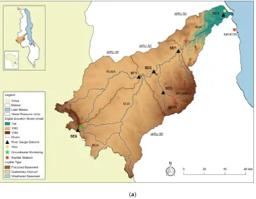
2.1. Study Area

The Bua river originates on the western border of Malawi and flows in a northeasterly direction

through Central Malawi to its outflow into Lake Malawi (Figure1a). The Bua is joined by five major

tributaries (Mphelele, Kasangadzi, Rusa, Ludzi and Namitete) and has numerous minor tributaries. It

has a catchment area of 10,658 km2which is approximately 186 km in length and its width varies from

The catchment comprises three distinct hydrological zones; the flat plateau, steep slopes on the

highland which rise from the plateau and the rift valley escarpment, and the lakeshore plain [30]. The

plateau is generally at 1000–1100 m above sea level (masl). Towards the southwest are the Mchinji mountains which rise to over 1750 masl. Towards the west, where the river meets the lakeshore plain, the catchment drops rapidly through a series of steep slopes. High levels of sedimentation occur at the lakeshore plain as the gradient becomes gentle.

The Bua catchment is assigned Water Resource Area (WRA) 5 within the National Water Resources

Master Plan (NWRMP) of Malawi [31]. WRA 5 is subdivided into four water resource units (WRUs)

named 5C, 5D, 5E and 5F (Figure1a). Both WRAs and WRUs are based on river basin boundaries.

WRA 5 lies within the administrative districts of Mchinji, Kasungu, Nkhotakota, Lilongwe, Dowa and Ntchisi.

Land use in WRA 5, as shown in Figure1c, mainly comprises cropland; arable agriculture of

mainly maize crops and tobacco, and forest land; including Mchinji Forest Reserve and Kasungu

National Park to the west, and Nkhotakota Game Reserve to the far east [32]. Wetlands or dambos

are also scattered throughout the catchment. These wetlands become saturated in the wet season and

provide a good source of water in the dry season [33]. The dambos are generally considered to drain

the plateau area [30].

The climate of WRA 5 can be generally represented as sub-tropical [31]. The climate is divided into

three weather variations; the warm wet season (1 November–30 April); the cool dry season (1 May–31 August); and the hot dry season (1 September–31 October), however, it’s generally accepted to be

bimodal referring to the wet season and the dry season [31]. Over 95% of the annual rainfall falls in the

warm wet season or rainy season. The exact length of the wet season varies depending on the location

within Malawi, reported to end in March in the south of the country, and April/May in the north [34].

No average annual rainfall or temperature values were available for the wet and dry season. The

average annual rainfall for WRA 5 is 897 mm, with a range of 800–1000 mm [33]. The average annual

temperature in WRA 5 ranges from 20 to 24◦C [33].

Water 2019, 11, x FOR PEER REVIEW 4 of 18

mountains which rise to over 1750 masl. Towards the west, where the river meets the lakeshore plain, the catchment drops rapidly through a series of steep slopes. High levels of sedimentation occur at the lakeshore plain as the gradient becomes gentle.

The Bua catchment is assigned Water Resource Area (WRA) 5 within the National Water Resources Master Plan (NWRMP) of Malawi [31]. WRA 5 is subdivided into four water resource units (WRUs) named 5C, 5D, 5E and 5F (Figure 1a). Both WRAs and WRUs are based on river basin boundaries. WRA 5 lies within the administrative districts of Mchinji, Kasungu, Nkhotakota, Lilongwe, Dowa and Ntchisi.

Land use in WRA 5, as shown in Figure 1c, mainly comprises cropland; arable agriculture of mainly maize crops and tobacco, and forest land; including Mchinji Forest Reserve and Kasungu National Park to the west, and Nkhotakota Game Reserve to the far east [32]. Wetlands or dambos are also scattered throughout the catchment. These wetlands become saturated in the wet season and provide a good source of water in the dry season [33]. The dambos are generally considered to drain the plateau area [30].

The climate of WRA 5 can be generally represented as sub-tropical [31]. The climate is divided into three weather variations; the warm wet season (1 November–30 April); the cool dry season (1 May–31 August); and the hot dry season (1 September–31 October), however, it’s generally accepted

to be bimodal referring to the wet season and the dry season [31]. Over 95% of the annual rainfall falls in the warm wet season or rainy season. The exact length of the wet season varies depending on the location within Malawi, reported to end in March in the south of the country, and April/May in the north [34]. No average annual rainfall or temperature values were available for the wet and dry season. The average annual rainfall for WRA 5 is 897 mm, with a range of 800–1000 mm [33]. The average annual temperature in WRA 5 ranges from 20 to 24 °C [33].

(a)

(b) (c)

Figure 1. (a) Location of Malawi in Africa (insert), location of the Bua catchment in Malawi (insert) and digital elevation model of the Bua catchment (WRA 5) with rivers, river gauges, weir, rainfall stations and groundwater monitoring; (b) aquifer type map [35]; (c) land use map [32].

Malawi’s groundwater occurrence is classified into three hydrogeological domains or aquifer

types; (1) alluvial aquifers, (2) sedimentary aquifers and (3) basement aquifers. The sedimentary aquifers are subdivided into semi consolidated and consolidated aquifers, and the basement is subdivided into weathered and fractured aquifers [31]. Figure 1b shows the aquifer types in WRA 5. The basement aquifer considered one of Malawi’s major aquifers underlays most of the Bua

catchment [35]. In the west, the weathered basement is present over most of the plateau area and fractured basement occurs in the area of the Mchinji Forest Reserve. In the east lakeshore plain, the basement is overlain by the other major aquifer type, the alluvium aquifer with some pockets of the fractured basement also present [35]. There has been little published work on the hydrogeology and soils of the Bua catchment, however, a bulletin from 1983 presents details of the soil’s patterns and

the hydrogeological conditions of the weathered basement aquifer of a plateau area [30].

2.2. Data

This study focused on data from six river gauges within the Bua catchment (Table 1). Other gauges do exist, however, there was no data available for them. Four gauges monitor the main Bua river (5C1, 5D1, 5D2 and 5E6) which is a regulated river with a weir located downstream of gauge 5C1. Photos of the weir taken January 2019 and are provided in the Supplementary Material, Figure S1. The Rusa river, a major tributary of the Bua, is monitored by a fifth gauge, 5F1, and the Mtiti river (a tributary to the Kasangadzi river) is monitored by the final gauge, 5D3. Daily flow rate data were available for each gauge as follows; 5C1 (1957–2009), 5D1 (1958–2007), 5D2 (1953–2007), 5D3 (1958–

2003), 5E6 (1970–2008) and 5F1 (1964–2005). Data coverage appears substantial ranging from 38–52 years, however, it is expected to have missing values throughout. Data were obtained from the Surface Water Division of the Department of Water Resources of Malawi.

Where possible, rainfall and groundwater data in the vicinity of the river gauges were also examined to provide support for the BFI analysis. Daily rainfall data for Nkhota station (18 km away from gauge 5C1 in a southeasterly direction) and Mponela station (13 km away from 5D3 in a southwesterly direction) were used. Stations are managed by the Department of Meteorological Services who provided the data. The rainfall data is of very good coverage with minimal missing values. Groundwater levels are monitored in WRA 5 via four monitoring boreholes, constructed around 2009/2010. The boreholes are managed by the Groundwater Division of the Department of Water Resources who provided the data. Only one of the monitoring boreholes, at Mchinji Water Office (GN196), had enough data coverage (2009–2013) to examine.

Figure 1.(a) Location of Malawi in Africa (insert), location of the Bua catchment in Malawi (insert) and digital elevation model of the Bua catchment (WRA 5) with rivers, river gauges, weir, rainfall stations and groundwater monitoring; (b) aquifer type map [35]; (c) land use map [32].

Malawi’s groundwater occurrence is classified into three hydrogeological domains or aquifer types; (1) alluvial aquifers, (2) sedimentary aquifers and (3) basement aquifers. The sedimentary aquifers are subdivided into semi consolidated and consolidated aquifers, and the basement is subdivided into

weathered and fractured aquifers [31]. Figure1b shows the aquifer types in WRA 5. The basement

aquifer considered one of Malawi’s major aquifers underlays most of the Bua catchment [35]. In the

west, the weathered basement is present over most of the plateau area and fractured basement occurs in the area of the Mchinji Forest Reserve. In the east lakeshore plain, the basement is overlain by the other major aquifer type, the alluvium aquifer with some pockets of the fractured basement also

present [35]. There has been little published work on the hydrogeology and soils of the Bua catchment,

however, a bulletin from 1983 presents details of the soil’s patterns and the hydrogeological conditions

of the weathered basement aquifer of a plateau area [30].

2.2. Data

This study focused on data from six river gauges within the Bua catchment (Table1). Other gauges

do exist, however, there was no data available for them. Four gauges monitor the main Bua river (5C1, 5D1, 5D2 and 5E6) which is a regulated river with a weir located downstream of gauge 5C1. Photos of the weir taken January 2019 and are provided in the Supplementary Material, Figure S1. The Rusa river, a major tributary of the Bua, is monitored by a fifth gauge, 5F1, and the Mtiti river (a tributary to the Kasangadzi river) is monitored by the final gauge, 5D3. Daily flow rate data were available for each gauge as follows; 5C1 (1957–2009), 5D1 (1958–2007), 5D2 (1953–2007), 5D3 (1958–2003), 5E6 (1970–2008) and 5F1 (1964–2005). Data coverage appears substantial ranging from 38–52 years, however, it is expected to have missing values throughout. Data were obtained from the Surface Water Division of the Department of Water Resources of Malawi.

Where possible, rainfall and groundwater data in the vicinity of the river gauges were also examined to provide support for the BFI analysis. Daily rainfall data for Nkhota station (18 km away from gauge 5C1 in a southeasterly direction) and Mponela station (13 km away from 5D3 in a southwesterly direction) were used. Stations are managed by the Department of Meteorological Services who provided the data. The rainfall data is of very good coverage with minimal missing values. Groundwater levels are monitored in WRA 5 via four monitoring boreholes, constructed

around 2009/2010. The boreholes are managed by the Groundwater Division of the Department of

Water Resources who provided the data. Only one of the monitoring boreholes, at Mchinji Water Office

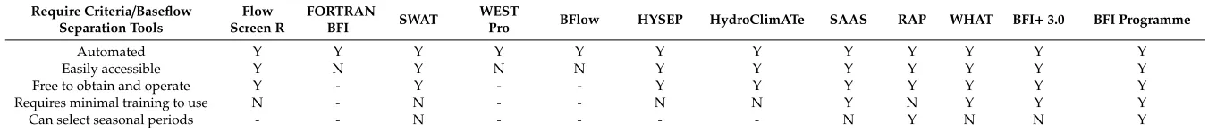
Table 1.Evaluation of baseflow separation tools against required criteria.

Require Criteria/Baseflow Separation Tools

Flow Screen R

FORTRAN

BFI SWAT

WEST

Pro BFlow HYSEP HydroClimATe SAAS RAP WHAT BFI+3.0 BFI Programme

Automated Y Y Y Y Y Y Y Y Y Y Y Y

Easily accessible Y N Y N N Y Y Y Y Y Y Y

Free to obtain and operate Y - Y - - Y Y Y Y Y Y Y

Requires minimal training to use N - N - - N N Y N Y Y Y

Can select seasonal periods - - N - - - - N Y N N Y

2.3. Decision Procedure for Selection of Baseflow Separation Method and Implementation Tool

Baseflow separation was selected to analyze the river data and determine BFI. Baseflow separation is categorized into graphical methods which are performed manually, and filtering methods which are

automatically performed by a computer. [36]. There are a wide variety of filtering methods available,

and a significant number of computer programs to implement the chosen method [37]. Although there

is subjectivity involved in selecting an appropriate filtering method and an associated tool to implement

it, merit holds in use of any of them as long as the use is consistent throughout the study [6,15,37]. The

decision to select a filtering method and implementation tool is generally based on the criteria required for the study.

In this study, the selection of an appropriate implementation tool took precedence over the selection of a filtering method. The tool was required to meet certain criteria to allow the exchange of knowledge with the Government of Malawi. The tool needed to be automated, easily accessible, free to obtain and operate, require minimal training to use and capable of selecting seasonal periods from input data to quantify BFI. Several tools were evaluated against the required criteria including Flow Screen

package for R [38], Formula Translation (FORTRAN) BFI program [39], Soil and Water Assessment Tool

(SWAT) [40], Water Engineering Time Series PROcessing Tool (WEST PRO) [41], web-based BFlow [42],

HYSEP [43], HydroClimATe: hydrologic and climate analysis toolkit [44], Streamflow Analysis and

Assessment Software (SAAS) [45], River Analysis Package (RAP) [46], Web-based Hydrograph Analysis

Tool (WHAT) [47], BFI+3.0 of Hydro Office [48] and the BFI programme [6]. The evaluation assessment

is presented in Table1. As the BFI Programme [6] met all of the criteria it was selected for analysis.

The BFI programme is an excel based tool developed by Martin Morawietz at the Department of Geosciences in the University of Oslo, Norway. It was originally prepared for the textbook;

Hydrological Drought-Processes and Estimation Methods for Streamflow and Groundwater [6]. It is

free to download on the European Drought Centre websitehttp://europeandroughtcentre.com/. The

textbook provides working examples of how to use the tool. The tool implements the filtering method

called the ‘smoothed minima procedure’ [21]. It uses smoothing and separation techniques to process

a river hydrograph. Daily river flow data is partitioned into 5-day increments and the minimum

flow in each period is identified [49]. Turing points are identified in the series of minimum flows and

connected to draw the baseflow hydrograph. The precise details of the procedure are provided in the

Low Flow Studies Report No 3 by the Institute of Hydrology [21] and by Wahl [39].

2.4. Baseflow Separation Steps

The raw river data were screened prior to baseflow separation to identify the periods of missing data. Before proceeding to analysis, there were two options available to deal with the missing data; (1) infill the missing data or (2) ignore the missing data and analyze only the raw data. Although there

are merits to infilling data [50,51], most studies agree with the recommendation by Ladson et al. [52]

that BFI should be determined from raw data only [20,23,53,54]. As such, this study did not infill data

and analyzed the raw river flow data only. To do this, the flow data were prepared by dividing into

periods of non-missing values [52].

The assessment periods selected were annual and seasonal periods defined by months. The annual period was taken as the hydrological year in Malawi as used by the Government of Malawi Water Resources Department and coincides with the start of the wet season and runs to the end of the dry season (1 November–31 October). The seasonal periods selected were the wet season defined as 1 November–30 April, and the dry season defined as 1 May–31 October. These periods are based on the weather variations recognized in Malawi and used in water resources assessments by the

Water Resources Department [55] and the country’s national irrigation master plan and investment

framework [56].

(1) The baseflow separation was performed for each year of river data (1957–2009) producing a separate annual BFI value for each year where there was enough data in the period. It is commonly recommended in the literature to determine the long-term BFI which uses all the data

successively [6,15], however here, it was not possible due to missing data. The mean annual BFI

was therefore determined based on the individual years;

(2) The baseflow separation was performed for each season of data (1957–2009) in the same manner

as the annual period described above;

(3) The total flow, baseflow and surface runoffflow from each baseflow separation were summed for

each period;

(4) Descriptive statistics (average, maximum and minimum, standard deviation and coefficient of

variation) were determined for the annual and seasonal periods.

2.5. Statistical Trend Analysis

The non-parametric Mann-Kendall (MK) statistical test [57,58] was used to identify if the BFI results

had statistically significant increasing or decreasing trends. The test is prominently used in hydrology

studies. For example, it is popular when identifying trends in streamflow [50,59–61], baseflow [50],

BFI [4,62,63] and the vertical exchange fluxes between streambeds and connected aquifers [64]. It is

also widely applied in identifying trends in rainfall [59,60]. Application of non-parametric testing is

appropriate due to hydrological data not being normally distributed [61]. One of the main advantages

of the MK test is that it is insensitive to missing data, which was a key challenge with the data in this study.

The hypothesis for the test, H0, was defined as ‘there is no trend in the data’, and the alternative

hypothesis, Ha, was defined as ‘there is a trend in the data’. If thep-value calculated was lower than

the significance level, the H0 was rejected and the alternative Ha accepted, and a trend was indicated.

If thep-value was greater than the significance level, no trend was indicated. The significance level is

referred to as a Type 1 error and is the probability of rejecting the null hypothesis when it is true [61].

The direction of the trend was indicated by the test statistic, S, where a negative S value indicates a declining trend and a positive S value indicates an increasing trend. Details of the MK equations can

be found in the literature [58].

The selection of the test parameters is important in statistical testing as they have a direct impact on the resulting trend. In this study, the following parameters were selected for the MK test; the ‘exact p’ method was used, the significance level was set to 0.01 (or 1%) and the equations were set to ignore missing data. Further, the ‘normal’ MK test was selected over the ‘seasonal’ MK test. Due to the decision not to infill data in this study, the BFI data was partitioned into annual and seasonal periods and as such the normal MK was applicable. If the data had been infilled, and there was no need to partition the data, the use of the seasonal MK test would have allowed comparison of the seasonal

periods. The statistical programme XLSTAT, available atwww.xlstat.comwas used to perform the MK

test [65].

3. Results and Discussion

3.1. Annual and Seasonal BFI Analysis Coverage

Annual and seasonal BFI was calculated for gauges 5C1, 5D1, 5D2, 5D3, 5E6 and 5F1. The results

of the analysis for 5C1 are presented in Table2and the results of the other gauges are presented in

Table 2.Results of the annual and seasonal BFI (base flow index) analysis (tabular) for the Bua River, gauge station 5C1, 1957–2009 (52 years).

Period Annual BFI

Wet Season

BFI

Dry Season

BFI

Period Annual BFI

Wet Season

BFI

Dry Season

BFI

1957/1958 - - 0.94 1983/1984 - -

-1958/1959 0.66 0.65 0.85 1984/1985 - -

-1959/1960 0.53 0.48 0.96 1985/1986 - 0.80

-1960/1961 - 0.44 - 1986/1987 0.81 0.80 0.99

1961/1962 0.83 0.81 0.91 1987/1988 0.62 0.58 0.95

1962/1963 - - 0.99 1988/1989 - -

-1963/1964 0.77 0.75 0.98 1989/1990 0.77 0.75 0.92

1964/1965 0.79 0.77 0.96 1990/1991 0.76 0.74 0.97

1965/1966 - 0.69 - 1991/1992 0.43 0.41 0.87

1966/1967 0.48 0.40 0.94 1992/1993 - 0.50

-1967/1968 0.58 0.54 0.83 1993/1994 - - 0.95

1968/1969 - - 0.81 1994/1995 0.60 0.60 0.91

1969/1970 - - - 1995/1996 0.54 0.53 0.84

1970/1971 - - - 1996/1997 0.76 0.75 0.89

1971/1972 - 0.64 - 1997/1998 0.90 0.90 0.87

1972/1973 - 0.47 - 1998/1999 0.76 0.74 0.92

1973/1974 0.68 0.62 0.94 1999/2000 0.75 0.73 0.87

1974/1975 0.72 0.72 0.99 2000/2001 - - 0.95

1975/1976 0.69 0.61 0.95 2001/2002 0.94 0.88 0.98

1976/1977 0.81 0.77 0.99 2002/2003 - 0.85

-1977/1978 - - 0.91 2003/2004 - - 0.99

1978/1979 0.80 0.76 0.99 2004/2005 0.84 0.82 0.92

1979/1980 - 0.65 - 2005/2006 0.90 0.82 0.98

1980/1981 0.75 0.71 0.99 2006/2007 0.87 0.81 0.96

1981/1982 - - - 2007/2008 0.92 0.87 0.99

1982/1983 - 0.64 - 2008/2009 0.88 0.81 0.99

- denotes no BFI determined due to insufficient data in that period.

As expected, the river data was characterized by missing values and this was seen across all datasets. This meant it was not possible to determine a BFI for all periods. To quantify the coverage of analysis, the number of periods for which a BFI was determined was counted and converted to a

percentage based on the number of years of data (Table3). For example, for 5C1, a BFI was determined

for 30 full annual data periods, 39 wet seasons, and 37 dry seasons which equates to 58%, 75% and 71 % coverage for the respective periods. Data for each gauge ranged from 38 to 52 years and the percentage of coverage for each period (annual, wet and dry season) was consistently over 50%, with

some periods as high as 80% coverage (Table3). The results show, despite the sporadic nature of river

flow data in Malawi, that such datasets can be analyzed to extract observations on baseflow. This is an important finding for Malawi and countries which hold similar datasets. They can begin to utilize such datasets and assess baseflow using minimal labor and financial resources.

Table 3.Percentage of data coverage in annual and seasonal BFI analysis for the gauges in WRA 5.

Gauge ID

River Name

Period of Data Coverage

No of Years of Available Data; No of Annual, Wet Season, Dry Season Periods with Data

Annual Wet Season

Dry Season

5C1 Bua 1957–2009 52; 30, 39, 37 58% 75% 71%

5D1 Bua 1958–2007 49; 25, 29, 31 51% 59% 63%

5D2 Bua 1953–2005 52; 34, 42, 35 65% 81% 67%

5D3 Mtiti 1958–2003 45;27, 30, 36 60% 67% 80%

5E6 Bua 1970–2008 38; 23, 27, 26 61% 61% 68%

5F1 Rusa 1964–2005 41; 24, 28, 27 59% 68% 66%

3.2. Average Annual BFI

Average annual BFI for the gauges were determined based on the BFI analysis results in Section3.1.

Traditionally BFI has been determined on an annual basis. This study found high average annual BFIs for the gauges located on the lower elevation reaches of the Bua; 0.74 for 5C1, 0.75 for 5D1 and 0.76 for 5D2. This indicates that the river has a moderately high baseflow component of approximately 74–76% of the total annual river flow in the lower catchment. This finding is consistent with the annual BFI of 0.71 for 5C1 and 0.86 for 5D1 sourced from the HYDSTRA system in use by the Malawi Surface

Water Division [33]. It also matches BFIs reported by Smith-Carington [30] of 0.85 (5D1) and 0.86 (5D2).

Previous studies by UNESCO [15] and Beck et al. [16] reported similar annual BFI for Malawi in the

range of 0.6 to 0.7 and 0.6 to 0.8 respectively. A moderately high baseflow was also found for 5F1 on the Rusa with a BFI of 0.80, or 80% of the total annual river flow which compares with a BFI of 0.81 from HYDSTRA.

In contrast, lower BFI values were found for the gauges located at higher elevations in the catchment. A BFI of 0.54 was found for 5E6, the highest gauged reach of the Bua. This doesn’t match the BFI of 0.74 found from HYDSTRA. Finally, 5D3 on the Mtiti found a BFI of 0.48. There was no BFI available from HYDSTRA. Comparisons are provided for context only, it is important to bear in mind,

that it’s not generally recommended to compare BFIs across studies as different baseflow separation

techniques and different data lengths will produce different baseflow volumes and this will affect

the BFI [52]. Based on this study’s annual average values, the Bua, the Rusa and the Mtiti rivers are

considered perennial in nature with a stable flow regime.

3.3. Average Seasonal BFI (Wet and Dry Season)

Recent studies in BFI have sought to make seasonal adjustments, appreciating the variations that occur in baseflow both temporally and spatially and that annual BFI may not represent the true

picture [66]. This study presents the first findings on seasonal BFI in the Bua catchment. Average

seasonal BFI for the gauges was determined based on the BFI analysis results in Section3.1. The results

are presented in Figure2and Table4.

For all gauges assessed, the results found minimal difference between the annual and the wet

season BFI, however, in the dry season, all BFIs increased to over 0.80 (or 80% of the dry season flow

was attributed to baseflow) as shown in Figure2and Table4. For example, 5C1 had a BFI of 0.69 in

the wet season increasing to 0.94 in the dry season. The increase in dry season BFI is indicative of the catchment geology. As mentioned in the literature, a high BFI indicates permeable catchment conditions whereby the catchment is storing water during the wet season and discharging it to the

river during the dry season [6,17]. To support these BFI findings, it would have proved useful to

compare river levels to groundwater levels near each gauging station. Unfortunately, however, of the groundwater data available there was none suitable for such a comparison.

Water 2019, 11, x FOR PEER REVIEW 11 of 18

3.3. Average Seasonal BFI (Wet and Dry Season)

Recent studies in BFI have sought to make seasonal adjustments, appreciating the variations that occur in baseflow both temporally and spatially and that annual BFI may not represent the true picture [66]. This study presents the first findings on seasonal BFI in the Bua catchment. Average seasonal BFI for the gauges was determined based on the BFI analysis results in Section 3.1. The results are presented in Figure 2 and Table 4.

Figure 2. Results of annual and seasonal BFI analysis for the gauges in WRA 5 (graphical).

Table 4. Results of annual and seasonal BFI analysis for the gauges in WRA 5 (tabular).

Gauge ID (River) 5C1 (Bua) 5D1 (Bua) 5D2 (Bua) 5D3 (Mtiti) 5E6 (Bua) 5F1 (Rusa) Data record 1957–2009 1958–2007 1953–2005 1958–2003 1970–2008 1964–2005

ANNUAL

Average BFI 0.74 0.75 0.76 0.48 0.54 0.80 Minimum Average BFI 0.43 0.43 0.11 0.05 0.37 0.26 Maximum Average BFI 0.94 0.94 0.98 0.84 0.70 0.98 Standard Deviation 0.13 0.17 0.24 0.28 0.09 0.18

WET SEASON

Average BFI 0.69 0.74 0.74 0.45 0.46 0.46 Minimum Average BFI 0.40 0.41 0.11 0.05 0.25 0.25 Maximum Average BFI 0.90 0.93 0.98 0.77 0.90 0.90 Standard Deviation 0.14 0.17 0.22 0.26 0.13 0.13

DRY SEASON

Average BFI 0.94 0.93 0.84 0.83 0.90 0.89 Minimum Average BFI 0.83 0.55 0.55 0.00 0.47 0.61 Maximum Average BFI 0.99 1.00 1.00 1.00 0.98 1.00 Standard Deviation 0.05 0.11 0.11 0.23 0.12 0.10

For all gauges assessed, the results found minimal difference between the annual and the wet season BFI, however, in the dry season, all BFIs increased to over 0.80 (or 80% of the dry season flow was attributed to baseflow) as shown in Figure 2 and Table 4. For example, 5C1 had a BFI of 0.69 in the wet season increasing to 0.94 in the dry season. The increase in dry season BFI is indicative of the catchment geology. As mentioned in the literature, a high BFI indicates permeable catchment conditions whereby the catchment is storing water during the wet season and discharging it to the river during the dry season [6,17]. To support these BFI findings, it would have proved useful to compare river levels to groundwater levels near each gauging station. Unfortunately, however, of the groundwater data available there was none suitable for such a comparison.

0.00 0.10 0.20 0.30 0.40 0.50 0.60 0.70 0.80 0.90 1.00

5C1 (Bua) 5D1 (Bua) 5D2 (Bua) 5D3 (Mtiti) 5E6 (Bua) 5F1 (Rusa)

B ase Fl o w In d e x

Average Annual Average Wet Season Average Dry Season

Table 4.Results of annual and seasonal BFI analysis for the gauges in WRA 5 (tabular).

Gauge ID (River) 5C1 (Bua) 5D1 (Bua) 5D2 (Bua) 5D3 (Mtiti) 5E6 (Bua) 5F1 (Rusa)

Data record 1957–2009 1958–2007 1953–2005 1958–2003 1970–2008 1964–2005 ANNUAL

Average BFI 0.74 0.75 0.76 0.48 0.54 0.80

Minimum Average BFI 0.43 0.43 0.11 0.05 0.37 0.26

Maximum Average BFI 0.94 0.94 0.98 0.84 0.70 0.98

Standard Deviation 0.13 0.17 0.24 0.28 0.09 0.18

WET SEASON

Average BFI 0.69 0.74 0.74 0.45 0.46 0.46

Minimum Average BFI 0.40 0.41 0.11 0.05 0.25 0.25

Maximum Average BFI 0.90 0.93 0.98 0.77 0.90 0.90

Standard Deviation 0.14 0.17 0.22 0.26 0.13 0.13

DRY SEASON

Average BFI 0.94 0.93 0.84 0.83 0.90 0.89

Minimum Average BFI 0.83 0.55 0.55 0.00 0.47 0.61

Maximum Average BFI 0.99 1.00 1.00 1.00 0.98 1.00

Standard Deviation 0.05 0.11 0.11 0.23 0.12 0.10

Interestingly, from the wet season BFI results (Figure2), there are two gauges which don’t follow

the high BFI seen in the other gauges; the 5D3 (Mtiti) and the 5E6 (Bua). The lower wet season BFI of these gauges can be attributed to the spatial variations in geology and topography which control baseflow. For example, both gauges are located at elevations of 1200masl, compared to the much lower elevations of 550–1000 masl for the other gauges. 5E6 is located on the headwaters of the Bua and drains the entirety of the Mchinji Forest Reserve (Figure S3) and 5D3 drains part of the Dowa Hills (Figure S4).

There is considerable variability seen across all gauges in the BFI within the annual and wet

season periods shown by the minimum and maximum BFIs (Table4). The coefficient of variation

(CV) of the dry season BFI was low, compared to the annual and wet season BFI which was, as expected, much larger. For example, at gauge 5C1, the dry season CV was 6%, compared to the

annual CV of 18%, and the wet season of 20%. This difference in variability highlights the varying

behavior of baseflow. As mentioned in the literature, BFI is used in hydrology and hydrogeology

in a range of applications [6,18,19]. Where there are variations between annual and seasonal values,

as seen in these results, it is important to use the appropriate value as the use of an incorrect BFI could lead to inaccurate assessments. Several future scheme appraisals in Malawi would benefit from considering the seasonal BFI results of this study. For example, previous assessments for new investments in Malawi’s water sector, which have taken account of EFRs and thus BFI values. The Water Resources Investment Strategy (WRIS) project, under the National Water development Program

(NWDP), produced water resource assessments for the 17 WRAs in Malawi, including WRA 5 [33].

The project produced estimates for potential abstractable groundwater and sustainable surface water yield. Further, the National Irrigation Master Plan and Investment Framework (2014–2035), which sets out new investments for expansion of the irrigation sector in Malawi, is also centered around EFR, with one new dam proposed in the lower Bua catchment. It is presumed that these estimations have used annual BFI values which may lead to overestimation of available water resources. Seasonal variations are evidenced in this study and should be considered.

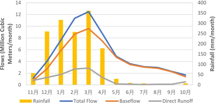
3.3.1. River Flow, Rainfall and Groundwater Patterns

Examining rainfall, river and groundwater patterns support the variation in wet and dry season

BFI found above. For example, river flow and rainfall patterns for gauge 5C1 are shown in Figure3.

The baseflow separation divided the daily river flow into its daily baseflow and daily surface runoff

components for each annual and seasonal period. Average monthly values for each flow component

were determined for the years with no missing data; 30 in total. Figure3shows the average monthly

Rainfall is high during the wet season (November–April) and in response the total river flow volume

and the direct runoffincreases. The baseflow also increases but to a much lesser extent. River flows

start to decrease after the peak river discharge in March. During the dry season (May–October), rainfall

and direct runoffare reduced to a minimum. However, the baseflow remains relatively stable and

sustains the river. The ratio of baseflow to total river flow is much higher in the dry season than in the wet season, thus resulting in a higher BFI. This pattern is considered generally representative of the

other gauges in the catchment.Water 2019, 11, x FOR PEER REVIEW 13 of 18

Figure 3. Average monthly flow volumes (total flow, baseflow, direct runoff), for the Bua River, Gauge 5C1, 1957–2009. Rainfall data for Nkhota station, 1960–2009.

There was not enough groundwater monitoring data available in the vicinity of gauge 5C1 for analysis. However, groundwater monitoring data at Mchinji Water Office (2009–2013), located 2 km from gauge 5E6 and at the same topographical elevation did have enough data. The data shows seasonal fluctuations in groundwater levels in line with the rainfall and river patterns above (Figure 4).

Figure 4. Daily rainfall (at Mchinji Boma) and sporadic groundwater levels (at Mchinji Water Office, GN196), located 2 km from the Bua River, Gauge 5E6, 2009–2013.

3.3.2. Comments on the Source of Baseflow

The baseflow separation approach used in this study assumes that baseflow is derived entirely from groundwater discharge from the aquifer, however, other stored sources can also contribute. The true source of baseflow is impossible to distinguish from baseflow separations alone and would require detailed site investigations to map each flow path [2]. It may be useful to provide some comments on the expected source of baseflow.

Based on the presence of aquifers identified through the literature and geological maps, we conceptualize that groundwater discharge from the local aquifers is the main contributor to baseflow during the wet and dry seasons. For example, an alluvium aquifer is present in the downstream reach of the Bua (5C1) and fractured basement dominates the entire upper catchment of the Bua (5E6) presenting good conditions for water to discharge to the river. Weathered basement aquifers

0 50 100 150 200 250 300 350 400 0 2 4 6 8 10 12 14

11月 12月 1月 2月 3月 4月 5月 6月 7月 8月 9月 10月

R ai n fal l (m m /m o n th ) Fl o ws (M ill io n Cu b ic M e te rs/m o n th )

Rainfall Total Flow Baseflow Direct Runoff

0 1 2 3 4 5 6 7 8 9 0 10 20 30 40 50 60 70 80 90

2009/10/9 2010/1/9 2010/4/9 2010/7/9 2010/10/9 2011/1/9 2011/4/9 2011/7/9 2011/10/9 2012/1/9 2012/4/9 2012/7/9 2012/10/9 2013/1/9 2013/4/9 2013/7/9 2013/10/9 Gr

o u n d wat e r Level (m b e lo w gr o u n d ) R ai n fal l (m m /d ay )

Rainfall at Mchinji Boma Groundwater level at Mchinji Water Office, GN196

Figure 3.Average monthly flow volumes (total flow, baseflow, direct runoff), for the Bua River, Gauge 5C1, 1957–2009. Rainfall data for Nkhota station, 1960–2009.

There was not enough groundwater monitoring data available in the vicinity of gauge 5C1 for

analysis. However, groundwater monitoring data at Mchinji Water Office (2009–2013), located 2 km

from gauge 5E6 and at the same topographical elevation did have enough data. The data shows

seasonal fluctuations in groundwater levels in line with the rainfall and river patterns above (Figure4).

Water 2019, 11, x FOR PEER REVIEW 13 of 18

Figure 3. Average monthly flow volumes (total flow, baseflow, direct runoff), for the Bua River, Gauge 5C1, 1957–2009. Rainfall data for Nkhota station, 1960–2009.

There was not enough groundwater monitoring data available in the vicinity of gauge 5C1 for analysis. However, groundwater monitoring data at Mchinji Water Office (2009–2013), located 2 km from gauge 5E6 and at the same topographical elevation did have enough data. The data shows seasonal fluctuations in groundwater levels in line with the rainfall and river patterns above (Figure 4).

Figure 4. Daily rainfall (at Mchinji Boma) and sporadic groundwater levels (at Mchinji Water Office, GN196), located 2 km from the Bua River, Gauge 5E6, 2009–2013.

3.3.2. Comments on the Source of Baseflow

The baseflow separation approach used in this study assumes that baseflow is derived entirely from groundwater discharge from the aquifer, however, other stored sources can also contribute. The true source of baseflow is impossible to distinguish from baseflow separations alone and would require detailed site investigations to map each flow path [2]. It may be useful to provide some comments on the expected source of baseflow.

Based on the presence of aquifers identified through the literature and geological maps, we conceptualize that groundwater discharge from the local aquifers is the main contributor to baseflow during the wet and dry seasons. For example, an alluvium aquifer is present in the downstream reach of the Bua (5C1) and fractured basement dominates the entire upper catchment of the Bua (5E6) presenting good conditions for water to discharge to the river. Weathered basement aquifers

0 50 100 150 200 250 300 350 400 0 2 4 6 8 10 12 14

11月 12月 1月 2月 3月 4月 5月 6月 7月 8月 9月 10月

R ai n fal l (m m /m o n th ) Fl o ws (M ill io n Cu b ic M e te rs/m o n th )

Rainfall Total Flow Baseflow Direct Runoff

0 1 2 3 4 5 6 7 8 9 0 10 20 30 40 50 60 70 80 90

2009/10/9 2010/1/9 2010/4/9 2010/7/9 2010/10/9 2011/1/9 2011/4/9 2011/7/9 2011/10/9 2012/1/9 2012/4/9 2012/7/9 2012/10/9 2013/1/9 2013/4/9 2013/7/9 2013/10/9 Gr

o u n d wat e r Level (m b e lo w gr o u n d ) R ai n fal l (m m /d ay )

Rainfall at Mchinji Boma Groundwater level at Mchinji Water Office, GN196

Figure 4.Daily rainfall (at Mchinji Boma) and sporadic groundwater levels (at Mchinji Water Office, GN196), located 2 km from the Bua River, Gauge 5E6, 2009–2013.

3.3.2. Comments on the Source of Baseflow

detailed site investigations to map each flow path [2]. It may be useful to provide some comments on the expected source of baseflow.

Based on the presence of aquifers identified through the literature and geological maps, we conceptualize that groundwater discharge from the local aquifers is the main contributor to baseflow during the wet and dry seasons. For example, an alluvium aquifer is present in the downstream reach of the Bua (5C1) and fractured basement dominates the entire upper catchment of the Bua (5E6) presenting good conditions for water to discharge to the river. Weathered basement aquifers underlay much of the middle reaches (5D1 and 5D2) and may contain pockets of perched aquifers. Further, interflow is expected to contribute to baseflow across all gauges during the wet season, though will not be a major source in the dry season. Finally, Dambos will also contribute to baseflow during the wet season and at the beginning of the dry season. Water is temporarily stored in the dambos and released slowly at the beginning of the dry season whereby it discharges to the river. Once the dambos have

drained, the baseflow is maintained entirely from groundwater from the aquifers [30]. Dambos are

present in much of the plateau area and the Rusa catchment (5F1) and have been previously identified

as contributing to baseflow in the middle reaches of the Bua (5D1 and 5D2) [30].

3.4. Long Term Behavioral Changes in BFI—Statistical Trend Results

Detecting trends in BFI can help us understand the possible links between hydrological processes, anthropogenic activities and environmental changes. The MK test was used to identify increasing or

decreasing statistically significant trends in the BFI results obtained in Section3.1. The MK results

are presented in Table5. This study presents the first findings on detecting trends in BFI in the

Bua catchment.

Table 5.Mann Kendall statistical results for BFI for gauges in WRA 5.

Gauge ID (River) 5C1 (Bua) 5D1 (Bua) 5D2 (Bua) 5D3 (Mtiti) 5E6 (Bua) 5F1 (Rusa) Data record 1957–2009 1958–2007 1953–2005 1958–2003 1970–2008 1964–2005

ANNUAL

MK Statistic ‘S’ 151 −₁₆₆ −_{107 125} −₉₀ −₂₉

Trend (1% sig. level) Increasing Decreasing No trend Increasing No trend No trend WET SEASON

MK Statistic ‘S’ 241 −₂₁₄ −_{188 161} −₁₀₂ −₅₀

Trend (1% sig. level) Increasing Decreasing Decreasing Increasing No trend No trend DRY SEASON

MK Statistic ‘S’ 62 −₁₄₂ −_{82 16 4} −₁₇

Trend (1% sig. level) No trend No trend No trend No trend No trend No trend

An increasing trend in BFI in the annual and wet season data was found at 5C1 (Bua) and 5D3 (Mtiti), however, no trend was found in the dry season data. Increases in baseflow have previously been

linked to increases in groundwater levels as a result of prolonged increases in rainfall [3]. However, no

trends in rainfall were detected in the annual, wet or dry season data from nearby rainfall stations; Nkhota station (close to 5C1) from 1960–2009, and Mponela station (close to 5D3) from 1960–2003 (Table S6). In contrast, a decreasing trend in BFI for the annual and wet season data was found for 5D1 (Bua) and 5D2 (Bua), however, no trend was found in dry season data. Decreases in BFI could be linked to prolonged over-abstraction of groundwater. Declining groundwater levels have been reported in Malawi; however, sparse monitoring of groundwater levels lends to lack of evidence of such trends. The natural vegetation of the plateau area was reported as Miombo woodland but had been cleared for

cultivation in the 1980s which may have resulted in major changes to the hydrological cycle [30].

These findings suggest that long term behavioral changes have occurred in the annual and wet season baseflow at several gauges in the Bua catchment as described above. Based on the tests being conducted at a significance level of 1%, there is a 1% risk of being wrong or a confidence level of 99% in the results. The trend results should, however, be interpreted with caution as further work is recommended to quantify the magnitude of the trends and examine potential drivers for such changes

in baseflow behavior [61].

The above resultsprovide new evidence of temporal variations in baseflow in the Bua catchment. This will be of interest to the new National Water Resources Authority within the Malawi Government for catchment planning.

4. Conclusions

The main aim of this study was to demonstrate, using a case study, how to use sporadic river datasets to produce meaningful observations on temporal variations in baseflow. The findings can be summarized in terms of their contribution to knowledge.

4.1. Catchment Originality

This is the first study to quantify temporal variations in baseflow in the Bua catchment. Annually,

average BFIs>0.74 were found for gauges in the lower reaches of the catchment, with lower BFIs<0.54

found for gauges in higher reaches. Seasonally, minimal difference was found between the annual and

wet season BFI, however, baseflow increased in the dry season across all gauges with BFI all found to

be>0.80. Long term trends were found in the annual and wet season BFI indicating behavioral changes

in baseflow have occurred within the catchment. No trend was found in the dry season BFI. The source of baseflow is expected to be mainly groundwater discharge from the aquifers underlain the rivers, however, interflow and dambo storage may also play a role. An implication of these findings is that temporal variations in baseflow should be considered in future scheme appraisals in the catchment such as the proposed irrigation infrastructure. Further, the results should be included in catchment management plans set by the new National Water Resources Authority within the Malawi Government, to inform the seasonal allocation of water resources in the catchment.

4.2. Generic Relevance to the Reader and the Wider Research Community

Apart from the Bua catchment case study, this article serves as an important example for other gauged catchments in Malawi, and indeed other countries, which are required to assess variations in baseflow to underpin IWRM and SDG 6, but are faced with similar challenges of sporadic river data. Further research is now needed to quantify temporal variations in baseflow for all gauged catchments in Malawi. Our on-going baseflow research seeks to do this by using the approach demonstrated in this study.

Supplementary Materials: The following are available online athttp://www.mdpi.com/2073-4441/11/5/901/s1; Supplementary Material word document containing the following Figures and Tables.Figure S1. Pictures of the weir located on the Bua river downstream of gauge 5C1, taken January 2019 by Oliver Phiri;Figure S2. Results of the annual and seasonal BFI analysis (graphical) for the Bua River, gauge station 5C1, 1957–2009 (52 years); Figure S3. River gauge 5E6 on the Bua river, draining Mchinji Forest Reserve, Google Earth Image, February 2019; Figure S4. River gauge 5D3 on the Mtiti river, draining part of the Dowa Hills, Google Earth Image, February 2019; Table S1. Results of the annual and seasonal BFI analysis (tabular) for the Bua river, gauge station 5D1, 1958–2007 (49 years);Table S2. Results of the annual and seasonal BFI analysis (tabular) for the Bua river, gauge station 5D2, 1953–2005 (52 years);Table S3. Results of the annual and seasonal BFI analysis (tabular) for the Mtiti river, gauge station 5D3, 1958–2003 (45 years);Table S4. Results of the annual and seasonal BFI analysis (tabular) for the Bua river, gauge station 5E6, 1970–2008 (38 years);Table S5. Results of the annual and seasonal BFI analysis (tabular) for the Rusa river, gauge station 5F1, 1964–2005 (41 years);Table S6. Mann Kendall statistical results for rainfall stations in WRA 5; Nkhota (1960–2009) and Mponela (1960–2003).

Funding:This research was funded by the Scottish Government under the Scottish Government Climate Justice Fund Water Futures Programme, research grant HN-CJF-03 awarded to the University of Strathclyde (R.M. Kalin).

Acknowledgments:The authors would like to gratefully acknowledge our partners the Malawi Government, in particular, the Surface Water Division and the Groundwater Division of the Department of Water Resources, and the Department of Meteorological Services for providing data for this study. A specific thank you to those who helped to facilitate and process the data requests; Jolamu Nkhokwe, Grey Muthali, Yobu Ezra Kachiwanda and Adams Chavula from the Department of Meteorological Services, Piasi Kaunda from the Surface Water Division.

Conflicts of Interest: The authors declare no conflict of interest. The funders had no role in the design of the study; in the collection, analyses, or interpretation of data; in the writing of the manuscript, or in the decision to publish the results.

References

1. Brodie, R.; Sundaram, B.; Tottenham, R.; Hostetler, S.; Ransley, T.An Adaptive Management Framework for Connected Groundwater-Surface Water Resources in Australia; Bureau Rural Sciences: Canberra, Australia, 2007. 2. International Commission on Groundwater. Surface Water and Groundwater Interaction. InA Contribution to

the International Hydrological Programme; The United Nations Educational, Scientific and Cultural Organization (UNESCO): Paris, France, 1980.

3. Fetter, C.W.Applied Hydrogeology, 4th ed.; Lynch, P., Ed.; Prentice Hall Inc.: Upper Saddle River, NJ, USA, 2001. 4. Bosch, D.D.; Arnold, J.G.; Allen, P.G.; Lim, K.-J.; Park, Y.S. Temporal variations in baseflow for the Little

River experimental watershed in South Georgia, USA.J. Hydrol. Reg. Stud.2017,10, 110–121. [CrossRef] 5. Smakhtin, V.U. Low flow hydrology: A review.J. Hydrol.2001,240, 147–186. [CrossRef]

6. Tallaksen, L.M.; Van Lanen, H.A.Hydrological Drought: Processes and Estimation Methods for Streamflow and Groundwater; Elsevier: Amsterdam, The Netherlands, 2004; Volume 48.

7. International Hydrological Programme of UNESCO.Groundwater Resources Assessment under the Pressures of Humanity and Climate Changes GRAPHIC; UNESCO: Paris, France, 2006.

8. Mei, Y.; Anagnostou, E.N. A hydrograph separation method based on information from rainfall and runoff records.J. Hydrol.2015,523, 636–649. [CrossRef]

9. Chimtengo, M.; Ngongondo, C.; Tumbare, M.; Monjerezi, M. Analysing changes in water availability to assess environmental water requirements in the Rivirivi River basin, Southern Malawi.Phys. Chem. Earth Parts A/B/C2014,67, 202–213. [CrossRef]

10. Tallaksen, L. A review of baseflow recession analysis.J. Hydrol.1995,165, 349–370. [CrossRef]

11. Bloomfield, J.; Allen, D.; Griffiths, K. Examining geological controls on baseflow index (BFI) using regression analysis: An illustration from the Thames Basin, UK.J. Hydrol.2009,373, 164–176. [CrossRef]

12. Rassam, D.W.; Werner, A.Review of Groundwater-Surfacewater Interaction Modelling Approaches and Their Suitability for Australian Conditions; eWater Cooperative Research Centre: Canberra, Australia, 2008. 13. Capesius, J.P.; Arnold, L.R.Comparison of Two Methods for Estimating Base Flow in Selected Reaches of the South

Platte River, Colorado; US Geological Survey: Reston, VA, USA, 2012.

14. Turner, J.V.Estimation and Prediction of the Exchange of Groundwater and Surface Water: Field Methodologies, eWater Technical Report; eWater Cooperative Research Centre: Canberra, Australia, 2009.

15. UNESCO Southern Africa FRIEND IHP-V Project 1.1 Technical Documents in Hydrology No.15; UNESCO: Paris, France, 1997.

16. Beck, H.E.; van Dijk, A.I.J.M.; Miralles, D.G.; de Jeu, R.A.; Bruijnzeel, L.A.; McVicar, T.R.; Schellekens, J. Global patterns in base flow index and recession based on streamflow observations from 3394 catchments. Water Resour. Res.2013,49, 7843–7863. [CrossRef]

17. Gustard, A.; Bullock, A.; Dixon, J. Low Flow Estimation in the United Kingdom; Institute of Hydrology: Wallingford, UK, 1992.

18. Ngongondo, C.S. An analysis of long-term rainfall variability, trends and groundwater availability in the Mulunguzi river catchment area, Zomba mountain, Southern Malawi.Quat. Int.2006,148, 45–50. [CrossRef] 19. Hughes, D.A.; Hannart, P. A desktop model used to provide an initial estimate of the ecological instream

flow requirements of rivers in South Africa.J. Hydrol.2003,270, 167–181. [CrossRef]

21. Institute of Hydrology.Low Flow Studies Report No 3; Institute of Hydrology: Wallingford, UK, 1980. 22. Singh, S.K.; Pahlow, M.; Booker, D.J.; Shankar, U.; Chamorro, A. Towards baseflow index characterisation at

national scale in New Zealand.J. Hydrol.2019,568, 646–657. [CrossRef]

23. Zhang, J.; Song, J.; Cheng, L.; Zheng, H.; Wang, Y.; Huai, B.; Sun, W.; Qi, S.; Zhao, P.; Wang, Y.; Li, Q. Baseflow estimation for catchments in the Loess Plateau, China.J. Environ. Manag.2019,233, 264–270. [CrossRef] 24. Hudak, A.T.; Wessman, C.A. Deforestation in Mwanza District, Malawi, from 1981 to 1992, as determined

from Landsat MSS imagery.Appl. Geogr.2000,20, 155–175. [CrossRef]

25. Chitete, S. The Nation “Malawi Drying up”. Available online:https://mwnation.com/malawi-drying-up/

(accessed on 16 April 2019).

26. Sood, A.; Smakhtin, V.; Eriyagama, N.; Villholth, K.G.; Liyanage, N.; Wada, Y.; Ebrahim, G.; Dickens, C. Global Environmental Flow Information for the Sustainable Development Goals; International Water Management Institute (IWMI): Colombo, Sri Lanka, 2017; Volume 168.

27. Kumambala, P.G. Sustainability of Water Resources Development for Malawi with Particular Emphasis on North and Central Malawi. Ph.D. Thesis, University of Glasgow, Glasgow, UK, 2010.

28. Kambombe, O.; Odongo, V.; Mutua, B.; Wambua, R. Impact of climate variability and land use change on streamflow in lake Chilwa basin, Malawi.Int. J. Hydrol.2018,2, 364–370.

29. Houghton-Carr, H.; Fry, M.; Wallingford, U. The decline of hydrological data collection for development of integrated water resource management tools in Southern Africa.IAHS Publ.2006,308, 51.

30. Smith-Carington, A. Hydrological bulletin for the Bua Catchment: Water resource unit number 5. In Groundwater Section; Department of Lands, Valuation and Water: Lilongwe, Malawi, 1983.

31. Government of Malawi, T.National Water Resources Master Plan 2017. Main Report: Existing Situation; Government of Malawi: Lilongwe, Malawi, 2017.

32. Government of Malawi.Malawi Land Use Map; Forestry Commission: Lilongwe, Malawi, 2018.

33. Government of Malawi.Water Resources Investment Strategy. Component 1—Water Resources Assessment, Annex I(ii) for WRAs 5-10; Government of Malawi: Lilongwe, Malawi, 2011.

34. Government of Malawi.Final Report for consultancy services related to detailed design of the upgraded Kamuzu Barrage; Extracts from Main Report Chapters 4–11 related to Hydrology–Hydraulics–Water Demand; Ministry of Water Development and Irrigation: Lilongwe, Malawi, 2013.

35. Government of Malawi. Malawi Hydrogeological and Water Quality Map 2018; Ministry of Agriculture, Irrigation and Water Development: Lilongwe, Malawi, 2018.

36. Brodie, R.; Sundaram, B.; Tottenham, R.; Hostetler, S.; Ransley, T. An Overview of Tools for Assessing Groundwater-Surface Water Connectivity; Bureau of Rural Sciences: Canberra, Australia, 2007; Volume 133. 37. Eckhardt, K. A comparison of baseflow indices, which were calculated with seven different baseflow

separation methods.J. Hydrol.2008,352, 168–173. [CrossRef]

38. Dierauer, J.R.; Whitfield, P.H.; Allen, D.M. Assessing the suitability of hydrometric data for trend analysis: The “FlowScreen”package for R.Can. Water Resour. J./Revue Canadienne Resour. Hydriques2017,42, 269–275. [CrossRef]

39. Wahl, K.L.; Wahl, T.L. Determining the flow of comal springs at New Braunfels, Texas.Unknown1995,95, 16–17.

40. Arnold, J.G.; Moriasi, D.N.; Gassman, P.W.; Abbaspour, K.C.; White, M.J.; Srinivasan, R.; Santhi, C.; Harmel, R.; Van Griensven, A.; Van Liew, M.W. SWAT: Model use, calibration, and validation.Trans. ASABE2012,55, 1491–1508. [CrossRef]

41. Willems, P. A time series tool to support the multi-criteria performance evaluation of rainfall-runoffmodels. Environ. Model. Softw.2009,24, 311–321. [CrossRef]

42. Younghun Jung, Y.S.N.-I.W.; Lim, K.J. Web-Based BFlow System for the Assessment of Streamflow Characteristics at National Level.Water2016,8, 384. [CrossRef]

43. Sloto, R.A.; Crouse, M.Y.HYSEP: A Computer Program for Streamflow Hydrograph Separation and Analysis; US Department of the Interior, US Geological Survey: Reston, VA, USA, 1996.

44. Dickinson, J.E.; Hanson, R.T.; Predmore, S.K.HydroClimATe: Hydrologic and Climatic Analysis Toolkit; US Department of the Interior, US Geological Survey: Reston, VA, USA, 2014.

46. CRC for Catchment Hydrology. River Analysis Package (RAP) Brochure. 2003. Available online: https: //toolkit.ewater.org.au/Tools/RAP(accessed on 2 August 2018).

47. Lim, K.J.; Engel, B.A.; Tang, Z.; Choi, J.; Kim, K.-S.; Muthukrishnan, S.; Tripathy, D. Automated Web GIS Based Hydrograph Analysis Tool, WHAT 1. JAWRA J. Am. Water Resour. Assoc. 2005,41, 1407–1416. [CrossRef]

48. Gregor, B.BFI+3.0 Users’s Manual; Department of Hydrogeology, Faculty of Natural Science, Comenius University: Bratislava, Slovakia, 2010; 21p.

49. Combalicer, E.; Lee, S.; Ahn, S.; Kim, D.; Im, S. Comparing groundwater recharge and base flow in the Bukmoongol small-forested watershed, Korea.J. Earth Syst. Sci.2008,117, 553–566. [CrossRef]

50. St. Jacques, J.-M.; Sauchyn, D.J. Increasing winter baseflow and mean annual streamflow from possible permafrost thawing in the Northwest Territories, Canada.Geophys. Res. Lett.2009,36. [CrossRef]

51. Harvey, C.L.; Dixon, H.; Hannaford, J. Developing best practice for infilling daily river flow data. InRole of Hydrology in Managing Consequences of a Changing Global Environment, Proceedings of the BHS Third International Symposium, Newcastle, UK, 19–23 July 2010; British Hydrological Society: London, UK, 2010; pp. 816–823. 52. Ladson, A.R.; Brown, R.; Neal, B.; Nathan, R. A standard approach to baseflow separation using the Lyne

and Hollick filter.Aust. J. Water Resour.2013,17, 25–34. [CrossRef]

53. Hodgkins, G.A.; Dudley, R.W. Historical summer base flow and stormflow trends for New England rivers. Water Resour. Res.2011,47. [CrossRef]

54. Oki, D.S.Trends in Streamflow Characteristics at Long-Term Gaging Stations, Hawaii, U.S Geological Survey Scientific Investigations Report 2004-5080; US Department of the Interior, US Geological Survey: Reston, VA, USA, 2004.

55. Government of Malawi.Water Resources Investment Strategy. Component 1—Water Resources Assessment. Annex II—Surface Water; Government of Malawi: Lilongwe, Malawi, 2011.

56. Government of Malawi.National Irrigation Master Plan and Investment Framework; Ministry of Agriculture, Irrigation and Water Development: Lilongwe, Malawi, 2015.

57. Mann, H.B. Nonparametric tests against trend.Econ. J. Econ. Soc.1945, 245–259. [CrossRef] 58. Kendall, M.G.Rank Correlation Methods, 4th ed.; Griffin: London, UK, 1975.

59. Gumindoga, W.; Makurira, H.; Garedondo, B. Impacts of landcover changes on streamflows in the Middle Zambezi Catchment within Zimbabwe.Proc. Int. Assoc. Hydrol. Sci.2018,378, 43–50. [CrossRef]

60. Da Silva, R.M.; Santos, C.A.; Moreira, M.; Corte-Real, J.; Silva, V.C.; Medeiros, I.C. Rainfall and river flow trends using Mann-Kendall and Sen’s slope estimator statistical tests in the Cobres River basin.Nat. Hazards 2015,77, 1205–1221. [CrossRef]

61. Yue, S.; Pilon, P.; Cavadias, G. Power of the Mann-Kendall and Spearman’s rho tests for detecting monotonic trends in hydrological series.J. Hydrol.2002,259, 254–271. [CrossRef]

62. Techamahasaranont, J.; Shrestha, S.; Babel, M.S.; Shrestha, R.P.; Jourdain, D. Spatial and temporal variation in the trends of hydrological response of forested watersheds in Thailand.Environ. Earth Sci.2017,76, 430. [CrossRef]

63. Zhang, X.S.; Amirthanathan, G.E.; Bari, M.A.; Laugesen, R.M.; Shin, D.; Kent, D.M.; MacDonald, A.M.; Turner, M.E.; Tuteja, N.K. How streamflow has changed across Australia since the 1950s: Evidence from the network of hydrologic reference stations.Hydrol. Earth Syst. Sci.2016,20, 3947. [CrossRef]

64. Anibas, C.; Schneidewind, U.; Vandersteen, G.; Joris, I.; Seuntjens, P.; Batelaan, O. From streambed temperature measurements to spatial-temporal flux quantification: Using the LPML method to study groundwater-surface water interaction.Hydrol. Process.2016,30, 203–216. [CrossRef]

65. Addinsoft XLSTAT Statistical and Data Analysis Solution; XLSTAT: Long Island, NY, USA, 2019.

66. Zhang, J.; Zhang, Y.; Song, J.; Cheng, L. Evaluating relative merits of four baseflow separation methods in Eastern Australia.J. Hydrol.2017,549, 252–263. [CrossRef]