City, University of London Institutional Repository
Citation:
Perin, C., Wun, T., Pusch, R. and Carpendale, S. (2017). Assessing the
Graphical Perception of Time and Speed on 2D+Time Trajectories. IEEE Transactions on
Visualization and Computer Graphics, doi: 10.1109/TVCG.2017.2743918
This is the accepted version of the paper.
This version of the publication may differ from the final published
version.
Permanent repository link:
http://openaccess.city.ac.uk/18384/
Link to published version:
http://dx.doi.org/10.1109/TVCG.2017.2743918
Copyright and reuse: City Research Online aims to make research
outputs of City, University of London available to a wider audience.
Copyright and Moral Rights remain with the author(s) and/or copyright
holders. URLs from City Research Online may be freely distributed and
linked to.
City Research Online:
http://openaccess.city.ac.uk/
[email protected]
Assessing the Graphical Perception of Time and Speed on
2D+Time Trajectories
Charles Perin, Tiffany Wun, Richard Pusch, and Sheelagh Carpendale
STRAIGHT 2D+TIME TRAJECTORY CURVED 2D+TIME TRAJECTORY
(no encoding)
Ø
CONSTANT SPEED TIME ENCODING
SPEED ENCODING
VARYING SPEED
(no encoding)
Ø
(a)
SIZE Min Speed Max Speed Ø (no encoding)
(b)
(no encoding)
Ø COLORVALUEMin Time Max Time
(c)
COLOR VALUE
Min Speed Max Speed
SIZE Min Time Max Time
(d)
(no encoding)
Ø SEGMENTLENGTH
Time Unit Min Time Max Time
(e)
COLOR VALUE
Min Speed Max Speed
SEGMENT LENGTH Time Unit
Min Time Max Time
[image:2.612.85.542.151.280.2](f)
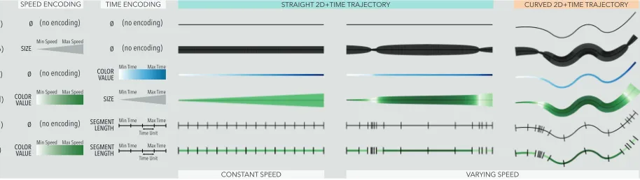
Fig. 1. Different encodings of time and speed for straight and curved 2D+time trajectories. Both constant speed and varying speed (two slow sections near the start and end, high speed in the middle) are shown. (a) Neither time nor speed are visually conveyed; (b) size (or stroke width) conveys speed; (c) color value conveys time elapsed; (d) color value conveys speed and size conveys time elapsed; (e) segment length (spacing between ticks) conveys time distribution, from which speed can be inferred (the closer two ticks, the slower); and (f) color value conveys speed on top of segment length. Results from studying nine visual encodings suggest that (e) and (f) are the best choices for conveying both time and speed and that (d) is the next best.
Abstract— We empirically evaluate the extent to which people perceive non-constant time and speed encoded on 2D paths. In our graphical perception study, we evaluate nine encodings from the literature for both straight and curved paths. Visualizing time and speed information is a challenge when the x and y axes already encode other data dimensions, for example when plotting a trip on a map. This is particularly true in disciplines such as time-geography and movement analytics that often require visualizing spatio-temporal trajectories. A common approach is to use 2D+time trajectories, which are 2D paths for which time is an additional dimension. However, there are currently no guidelines regarding how to represent time and speed on such paths. Our study results provide InfoVis designers with clear guidance regarding which encodings to use and which ones to avoid; in particular, we suggest using color value to encode speed and segment length to encode time whenever possible.
Index Terms—Trajectory visualization, visual encoding, movement data, graphical perception, quantitative evaluation.
1 INTRODUCTION
Temporal data is prevalent in many fields such as history, meteorology, finance, geography, industrial processes and social movements. The most common way of representing time is to assign it to one of the spatial axes using the positional variablesxorybecause position is the most powerful visual variable [55] – for example a line chart typically maps time to thex-axis. However, sometimes it is not possible to map time to position because positional variables are already encoding other dimensions of the data, such as geographical locations on a map or more abstract dimensions in a scatterplot.
In the simple example of travel, one could be interested in visualizing where one has travelled, where one is at a given point in time, and how time has passed while travelling. Typically, a 2D path drawn on a map would show the route taken, but might omit contextual details such as travel speed, allowable speed, or how long it takes to traverse a route.
• Charles Perin is with City, University of London and University of Calgary. E-mail: [email protected].
• Tiffany Wun, Richard Pusch, and Sheelagh Carpendale are with University of Calgary. E-mail:{twwun,rapusch,sheelagh}@ucalgary.ca.
This is the author version of the work
The literature is full of examples where encoding information about time and/or speed on these 2D paths, or2D+time trajectories, is impor-tant (see Figures 4, 6, and 7). Researchers and InfoVis designers have encoded speed and time along 2D paths using visual variables such as size (e.g., [1, 9, 10]), color brightness or value (e.g., [1, 9, 23, 32, 71]), and segment length (e.g., [10, 70]). Although InfoVis designers often have to decide how to visually encode time and speed information on 2D+time trajectories, so far no studies have been conducted to assess the relative interpretability of these visual encodings and no guidelines exist for helping designers in making such decisions.
To fill this gap, we studied thegraphical perception[20] of nine time and speed encodings for 2D+time trajectories (Figure 1(b–f) shows five of these encodings). We selected these nine encodings based on our review of the visual variables that have been used in the literature to encode time and speed. 18 participants performed two tasks (perceiving speed and perceiving time), for two path shapes (straight and curved), and for all nine encodings, multiple times. For simple straight or curved paths (no complex shape, sharp angles or loops), and when it is important to estimate the speed and/or time value at a point on the path, our results in terms of accuracy and completion time indicate that:
1. The best choices are either to encode speed with brightness/color value and time with segment length, or to encode both time and speed using segment length only.
2D+time trajectories range from very simple to very complex. Our results apply to the very simple cases, in situations where the shapes of the paths are either straight or smoothly curved. These results open the door to a wealth of opportunities for running studies towards developing a fuller understanding of how to best encode time and speed on 2D+time trajectories. In particular, now that we have identified encodings that should be avoided, future studies can build on this work and focus on encodings that perform well for new tasks and trajectory types.
2 BACKGROUND ANDRELATEDWORK
There exists a wide variety of techniques for representing time in visualization such as line graphs, small multiples, and animation (see [1, 6, 8] for comprehensive reviews). In this paper, we focus on a technique called time flattening. We first explain the space-time cube metaphor and time flattening. This provides a framework to describe 2D+time trajectories. Then, we survey the ways of encoding time and speed on 2D trajectories. Lastly, we discuss related graphical perception studies.
2.1 Space-Time Cube and Time Flattening
Spatio-temporal data in 2D consists of data points which have two spatial dimensions and a temporal dimension. When time cannot be mapped to eitherxory, it can be mapped to the other spatial dimension, z. This creates aspace-time cube[38], which refers to the treatment of time as a third dimension in addition to two spatial dimensions [54]. The space-time cube metaphor has often been taken literally to visualize 2D data in 3D, for example in geo-visualization (e.g., [34, 48, 50]) and for the visual analytics of movement data [4, 5, 7]. Bach et al. [8] clarify that“a space-time cube does not need to involve spatial data.” The space-time cube representation has in fact been used to visualize non-spatial, abstract data, such as in Configurable Spaces [44]. The 3D space-time cube, however, suffers from 3D visualizations problems, such as occlusion [75] and inconsistent perception across rotations [39]. Using the space-time cube conceptually instead of literally provides alternatives to 3D visualizations. Bach et al. [8] calltime-flatteningthe technique that “aggregates a space-time volume into a plane orthogonal to the time axis” [8, page 9]. The result is similar to the one of long exposure photography, where several frames of an image changing over time in a time interval are collapsed into a single image.
Time flattening an object’s 2D position over time creates a 2D+time trajectory, such as a travel itinerary on a map. For example, Minard’s comparison of Hannibal’s and Napoleon’s campaigns [58] in Figure 2 shows the 2D position of armies over time. In this example, the thick-ness of the 2D path encodes the size of the army. Neither time nor speed are visually encoded. In a visualization context, spatial 2D+time trajectories where conveying temporal information is important are prominent in, e.g., movement analysis [7] and eye tracking data [14]. Time-flattening non-spatial data also creates 2D+time trajectories. For example, in Hans Rosling’s famous TED talk [62], the dots of scatter-plots change position according to time. Dots follow trajectories in two non-spatial dimensions, such as lifespan and income. Similarly, Dim-pVis [46] shows 2D+time trajectories of abstract data for navigating in time via the direct manipulation of graphical elements in visualizations. In this paper, we focus on time-flattened 2D+time trajectories.
2.2 Encoding Time and Speed on 2D+time Trajectories
When looking at 2D+time trajectories, both the absolute time, and the relative speed can be of interest. Here, we describe the visual variables that have been used to encode time and speed on 2D+time trajectories.
Sizeis sometimes used to encode time on 2D+time trajectories [1]. Figure 3 (left) shows time being mapped to the size (or stroke-width) of the path. Bertin provides examples of using size for encodingmovement data [10] (see Figure 5(b)). Bach et al. [9] discussed encoding the duration between two consecutive events on a trajectory by varying the curve’s thickness. In that case, a thicker curve represents a long time interval between two events, which corresponds to a slow speed.
Color value/brightness(we refer tovaluein this paper) frequently
[image:3.612.313.551.48.255.2]encodes time on 2D+time trajectories [1]. Figure 3 (right) illustrates mapping time to brightness. Figure 4 showscolored time flattening[8], where each data item on aTime Curve[9] has been assigned a color
Fig. 2. Minard’s comparison of Hannibal’s second Punic war campaign (top) and Napoleon’s Russian campaign (bottom) [58].
Time Time
y
x t
y
[image:3.612.320.539.306.414.2]x t
Fig. 3. Encoding time on a 2D trajectory using line-width (left) and brightness (right). Reproduction from [1] with added Legends.
[image:3.612.330.540.466.592.2]Time
Fig. 4. Evolution of temperature over time using time curves [9]. The color of time points encodes their timestamp. Legend was added.
(a) (b) (c) (d)
[image:3.612.308.559.639.698.2]according to its timestamp. Time has also been color-coded on strokes to show the stroke order when writing Chinese characters [77], and in abstract graphs [23]. Value has also been used to encode speed, either in grayscale [32] or on a color ramp [18, 71] (see Figure 6 for an example created using Tableau). It is also common to map velocity in a vector field to a color ramp in flow visualization (e.g., [12, 73]).
Segment lengthhas been used intime geographyto create Linear
Cartograms. Linear Cartograms move spatial points on maps such that travel time between two points is encoded by the length of the link between these two points [13, 43, 64]. As a result, Linear Cartograms do not remain faithful to the spatial position – or 2D attributes – of data points. To solve this issue, Linear Cartograms with Fixed Vertex Positions [16] maintain the position of points, and instead, create sinu-soidal links whose length represents time between points. Visits [70] uses a similar approach: position along the horizontal axis represents time, while sizes of the circles encode duration. Bertin [10] proposed marking time units using ticks to convey both time and speed without distorting the 2D path: time ticks convey time elapsed, and spaces between ticks (i.e., segment lengths) convey speed (see Figure 5(c)). Bertin [10] used time ticks to convey speeds of ships on a map (see Fig-ure 7). He also proposed using segment length and size simultaneously to double encode speed, as shown in Figure 5(d). Arrows, which are often used to encode velocity in vector fields in flow visualization [51], could encode time/speed along a trajectory. Although we did not find an example of such, arrows would be similar to time ticks (segment length), except they would also provide direction along the trajectory.
Summary.Several visual variables (size, color value, and length)
have been used for encoding either the time or speed of 2D+time trajec-tories in time flattened visualizations. However, to our knowledge, no study has assessed the graphical perception of these visual encodings.
2.3 Studies on Graphical Perception
Graphical perception is “the visual decoding of the quantitative and qualitative information encoded on graphs” [19], or more generally, the ability to understand the visual encoding of information [53].
Graphical perception studies for statistical data graphics have a long history with studies of factors such as types of representations and shapes dating back to 1926 [26, 27, 33, 61]. Researchers in cartography have ranked the effectiveness of visual variables (e.g., [54, 65]). Sim-ilarly, in information visualization during the 1980s and early 1990s, Cleveland and McGill [19–22] and Spence [67] conducted graphical perception studies to experimentally rank visual variables. These stud-ies confirmed Bertin’s [10] rankings of visual variables according to their effectiveness for encoding nominal, ordinal, and quantitative data. This method has been used to study how people use bar charts, pie charts, scatterplots, and tables [52, 66, 68, 72] among others. It has been used to study changes of variable rankings when looking at large dis-plays [11,76], the perception of uncertainty in visualizations [15,37,63], and the perception of mean and error representations [24].
Guidelines that are derived from these studies provide guidelines about which encodings to use, thus inform to the grammar of visualiza-tion [78] and are used in automatic presentavisualiza-tion software [55, 56] such as Tableau. Our new graphical perception study adds guidance on how to best encode time and speed on 2D paths.
3 STUDYRATIONALE
Many factors could play a role in the graphical perception of time and speed on 2D+time trajectories, including:
• The choice of tasks participants are asked to perform.
• The 2D path, including its curvature, direction, length, range of angles (abrupt changes of direction), and crossings.
• The time function (ranges of speeds and time distributions). • The background, with its color and texture (e.g., a map). Our goal was to establish which visual encodings to use to encode time and speed on 2D+time trajectories. Therefore, we prioritized the number of encodings to study at the cost of constraining other factors in order to i) limit the influence of confounding factors; ii) ensure consistent difficulty between datasets and tasks; and iii) limit the duration of the experiment.
Speed
[image:4.612.317.569.50.135.2]10 30
Fig. 6. A dual color ramp encodes speed along the path of a bike ride.
La Havana
La Jamaica
Ocoa Puerto rico
LES ANTILLES
LES CANARIES
La Trinidad Caracas Cartagena
Fig. 7. Reproduction of Bertin’s [10] map where time ticks convey both the total travel time and the speed of a ship.
3.1 Choice of Tasks
Graphical perception tasks are often either value comparison tasks (e.g., [20, 41, 67]) or value estimation tasks (e.g., [61, 66]). We decided for the latter, specifically inverse lookup elementary tasks in Andrienko and Andrienko’s [6] task taxonomy for time-varying data.
In the TIMEtask, participants had to find the point on the trajectory that represents a certain amount of time elapsed (e.g., 50% of the total time). In the SPEED, task, they had to find the point where the speed is maximal or minimal. These two low-level tasks are often involved in compound higher-level real world tasks. For example, the SPEED
task could be used to determine where a cyclist was struggling up a hill or comparing where two race cars reach their maximum speed, since this involves finding points on a trajectory where speed is at its lowest or highest. To illustrate an example where the TIMEtask is useful, when conducting eye tracking experiments, it is helpful to know at which point in time a participant was looking at a particular feature in a visualization, or how long a participant took to find an object.
These standard tasks were well suited to our study for three reasons. First, the purpose of this study was to assess how people can quickly read time and speed (bottom-up process), as opposed to more complex tasks with higher cognitive load (such as comparing the speed of two segments). For this reason, we selected the simplest tasks that require reading information about time and speed, which lay the ground for studying more complex tasks [2]. Second, the same input method can be used to perform both time and speed related tasks (clicking a point on the path), limiting participants’ overhead of learning different input methods. Finally, time is monotonically increasing along the 2D path. This ensures that there is a unique correct answer for each task. Because speed is not monotonous, we used the task where participants have to find extrema as it ensures that there is a unique answer to each task.
3.2 Paths and Time Functions Generation
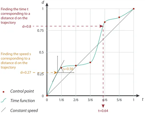
[image:4.612.315.568.173.270.2]t d
1
0.75
0.5
0.25
0
0 1/6 2/6 3/6 4/6 5/6 1
Time function
Constant speed Control point
d=0.8
d=0.27
t=0.64
s=0.56
Finding the time t corresponding to a distance d on the trajectory
[image:5.612.45.297.50.246.2]Finding the speed s corresponding to a distance d on the trajectory
Fig. 8. A sample time function. Control points are evenly distributed
along the time axist, but are assigned random, increasing heights along
the distance axisd. Shown are approximations for finding timetgiven
distance along the pathd, and the speed (i.e., tangent).
path shapes to only straight or smoothly curved. We included this factor because changes in curvature are common in 2D+time trajectories and may change the perception of visual encodings. We tested both straight paths and curved paths with a fixed direction from left to right, no sharp angles and no crossings (see Figure 1).
We generated curved paths using B-Splines with six control points to produce smooth curves with simple variations. We evenly spaced control points by 140px horizontally and assigned each a randomy value between -200 and 200px. We used a fixed increment for the xvalue of control points for two reasons: it ensures the path always travels from left to right, so thedirectionof the path is clear, and it ensures the path does not have loops or self-intersections. We fixed theycoordinate of control points to be in a 400px range so that the
maximum bounding box of the paths was 700×400px.
The constraints for curved paths informed the constraints for the straight ones, specifically to limit the confounding factor of pathlength. We determined the range of lengths for straight paths by generating one million curved paths. The distribution of their lengths was pseudo-normal and 86% of the lengths were in the range 750–1000px. Thus, we constrained the straight paths to have a random length in the range 750–1000px so that straight and curved paths had comparable lengths. We generated time functionsT:t7→d, witht∈[0,1]the time value, andd∈[0,1]the distance along the path fort. We used B-Splines with seven control points to generate time functions (see Figure 8). To ensureT are monotone increasing functions (the distance along the curve increases with time), we generated control points as follows: 1) create a setDof valuesdi∈D, with|D|=7,d0=0,d6=1, andd1...5
is a random value in[0,1]; 2) sort the values inDin ascending order; 3) create seven control points,C, with eachCi= (i/6,di). This results
in monotone increasing functions whose control points are evenly distributed along thetaxis, withT(0) =0 andT(1) =1.T are smooth functions with no sharp corners, but they can vary wildly with moments of extreme speed or slowness, depending on the values inD. To retrieve tgivend, we simply applyT−1, the inverse ofT. To retrieve the speed s(t)at(t,d), we find the slope of the tangent of the time function at
(t,d). BecauseT is monotonically increasing,s(t)∈[0,π/2]. Initially, approximately 40% of the generated time functions had
minimum or maximum speed att=0 ort=1, which would bias the
results for speed questions. To remove this bias, we constrained the time functions for speed-related tasks to have minimum and maximum speeds withint∈[0.03,0.97].
3.3 Choice of Encodings
While many encodings can be used to encode time and/or speed on 2D+time trajectories, we chose to study encodings that have been used in the literature to encode real-world data. As a result, we study the encodings that academics and practitioners in the field have considered appropriate to encode time and/or speed, which we presented in Sec-tion 2:size, colorvalue, and segmentlength. To refer to an encoding, our notation uses the letter S or T to indicate speed or time, followed by a icon showing its specific visual variable. For example, encoding speed using color value is referred to as
S
VALUE.We also studied both single encodings (either time or speed is en-coded using one visual variable) and double encodings (both time and speed are encoded using two visual variables). This decision was driven by two reasons. First, segment length conveys both time and speed (Figure 5). This made it a requirement to compare this encoding to encodings that also convey both time and speed, i.e., double encodings. Second, time and speed are dependant variables. Studying double en-codings made it possible to explore the effects of encoding one variable on top of the other and how these two visual variables may interact with each other. We call encodings that can show two data dimensions double encodings. This contrasts withredundant encodings[47] that show the same data dimension. For example, the double encoding
VALUE
S
T
LENGTH encodes speed using color value, and time using segment length. If speed or time is not encoded, we useS
ØorS
T
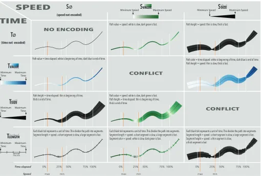
Ø.Figure 9 shows the nine studied encodings. They are combinations of encoding speed and/or time, using value, size, and length.
• Speed-only encodings: color value
S
VALUE, and sizeS
SIZE. • Time-only encodings: color valueS
VALUET
, size SIZES
T
and segmentlength
T
LENGTH.• Speed and time double encodings:
– Speed as color with time as size
S
VALUE SIZES
T
,– Speed as color with time as segment length
S
VALUET
LENGTH,– Speed as size with time as color
S
SIZES
VALUET
,– Speed as size with time as segment length
S
SIZET
LENGTH.3.3.1 Color Value
We picked two color ramps fromhttp://colorbrewer2.org/, using green for speed (
S
VALUE) and blue for time (S
VALUET
), in order to avoid confusion when changing from a time-color encoding to a speed-color encoding. Speed (S
VALUE):The color value at any point on the path conveys the speed at this point. A paler green means slower speed; a darker green means faster speed, no variations in color means constant speed.The
S
VALUEmapping function required particular attention. Wegener-ated 10 million time functions like Figure 8, and found that there was a pseudo-normal distribution of speeds (angles). Due to the difficulty in perceiving slight changes in color, we usedhistogram equalization, a technique which is recommended for lookup tasks [1] such as our SPEEDtask. Histogram equalization consists of subdividing the value range intonuniform bins and counting the number of data values in each bin. The color scale is sampled according to the cumulative fre-quencies of the bins, i.e., a bin containing many data values is attributed a bigger slice of the color ramp. Using histogram equalization ensured that the scale of colors reflected the data’s value distribution, and also improved discriminability of values, especially in high density regions.
Time (
S
VALUET
):The color value at any point conveys the time at this point. The palest blue means 0% of time elapsed; the darkest blue means 100% of time elapsed; a linear gradient change means linear time. In contrast toS
VALUE,S
VALUET
did not need histogram equalization asall values of time are shown equally.
3.3.2 Size
The visual variable size changes the thickness of the path.
Speed (
S
SIZE):The path thickness at any point conveys the speed at this point. A thinner path means slower speed; a thicker path means faster speed; no variation in thickness means constant speed.Time ( SIZE
S
TIME
SPEED
(speed not encoded)
Minimum Speed Maximum Speed Minimum Speed Maximum Speed
0% 25% 50% 75% 100%
0%
max min max min max min
25% 50%
Time elapsed
Speed
75% 100% 0% 25% 50% 75% 100%
CONFLICT
CONFLICT NO ENCODING
Path value = speed: white is slow, dark green is fast. Path height = time elapsed: thin is beginning of time, thick is end of time.
Path value = speed: white is slow, dark green is fast.
Each black tick represents a unit of time. This divides the path into segments. Segment length = speed: a short segment is slow, a large segment is fast. Segment color = speed: white is slow, dark green is fast.
Path color = time elapsed: white is beginning of time, dark blue is end of time. Path height = speed: thin is slow, thick is fast.
Path height = speed: thin is slow, thick is fast.
Each black tick represents a unit of time. This divides the path into segments. Segment length = speed: a short segment is slow, a large segment is fast. Segment height = speed: a thin segment is slow,
a thick segment is fast Path value = time elapsed: white is beginning of time, dark blue is end of time.
Path height = time elapsed: thin is beginning of time, thick is end of time.
Each black tick represents a unit of time. This divides the path into segments. Segment length = speed: a short segment is slow, a large segment is fast.
Ø
S
(time not encoded)
Ø
T
VALUE
S
Minimum Time MaximumTime
VALUE
T
SIZE
S
Minimum Time MaximumTime
SIZE
T
Minimum Time
Time Unit Maximum
Time
LENGTH
[image:6.612.58.568.47.392.2]T
Fig. 9. Time and speed encodings on 2D paths. Speed can be: not encoded (
S
Ø) or encoded usingvalue(S
VALUE) orsize(S
SIZE). Time can be: notencoded (
S
T
Ø) or encoded usingvalue(S
VALUET
),size(SIZES
T
), orlength(T
LENGTH). We tested all nine encodings that convey at least one of speed and time.3.3.3 Segment Length
We used the visual variable length by creating time ticks orthogonal to the path (similar to Figure 7). These ticks resemble Linear Cartograms with Fixed Vertex Positions [16], but they do not distort the path.
T
LENGTH is a particular encoding in that it conveys both time and speed.Speedcan be inferred by assessing a segment’s length. The space between two ticks represents the distance travelled in each of these time ”units”. A larger gap between two ticks means that more distance is covered within one time unit, implying faster speed. A smaller gap implies slower speed.
Timecan be inferred by assessing the distribution and frequency of ticks. Evenly distributed ticks means linear time. We chose to sample time at 23 evenly spaced intervals and to draw ticks at each resulting position on the path. We chose 23 ticks for two reasons: i) it is a sufficient number of ticks to indicate small and large trends in the data; and ii) it is prime, ensuring that no ticks will fall exactly on common milestones such as one-third or one-half of the time elapsed.
3.3.4 Null Encodings
Mapping speed or time to the null encoding means that this information is not explicitly encoded. Five of the nine encodings do not explicitely encode either speed (
S
Ø) or time ( ØS
T
).3.3.5 Double Encodings
Among the encodings shown in Figure 9, fourdouble encodespeed and time. These four encodings are
S
VALUE SIZES
T
,S
VALUET
LENGTH,S
SIZES
VALUET
,and
S
SIZET
LENGTH. We did not study theS
ØS
T
Ø encoding, which encodes neither speed nor time. Although such a condition can sometimes be used as a baseline, in our study, asking participants to assess time and speed without any indication would have resulted in a random baseline not suited for comparison.4 STUDY OFENCODINGS
The purpose of the study was to determine the differences between the nine visual encodings we presented, in performing time- and speed-related tasks on 2D+time trajectories.
4.1 Experimental Design
The three factors were ENCODING(the nine visual encodings), TASK
(TIMEand SPEED), and SHAPEof the path (STRAIGHTand CURVED). We used a within-participant design, where all participants perform the exact same trials. We counterbalanced ENCODINGand TASKin order to mitigate learning effects.
The experiment consisted of 9 encoding blocks. Each encoding block was split into two task blocks. Each task block consisted of training trials followed by 12 recorded repetitions (6 STRAIGHT, then 6 CURVED). A participant always performed the task blocks in the same order for all encoding blocks. To summarize, the experiment consisted
of 18participants×9 ENCODING×2 TASK(TIME, SPEED)×2
SHAPE(STRAIGHT, CURVED)×6repetitions=3888 trials.
4.2 Dataset and Tasks
We generated a dataset for measured trials. For all 36 (ENCODING
× TASK × SHAPE) combinations, we created six repetitions with
a 2D path, a time function, and a value the participant had to lo-cate on the path, each randomly generated. This resulted in 216 tu-ples{ENCODING,TASK,SHAPE, 2D path, time function, value}, that were used by all participants. For TIME, the values to locate were 25%, 50%, and 75% of the total elapsed time, with each value appearing twice. For SPEED, the values to locate wereminimumandmaximum, with each value appearing three times. Within each TASK×SHAPE
4.3 Dependent Measures: Time and Accuracy
For each trial, we measured the time participants took to complete the task and the error of their answers.
The error for each trial is the absolute value of the difference between a participant’s answer and the correct answer. Because all possible values of timet∈[0,1]are visible and encoded for TIME, this measure of error is consistent across TIMEtrials. In contrast, only a subset of speed valuess∈[0,π/2]are encoded for each SPEEDtrial, according to the time functionT. To ensure consistency of measure across SPEED
trials, we normalized the error measurement for each trial according to the minimum and maximum speed for the current trial:
error=
pAnswer−cAnswer max−min
, with
pAnswer the participant answer cAnswer the correct answer
min the trial minimum time or speed value
max the trial maximum time or speed value
Because for TIME, min=0 andmax=1 for all trials, error=
|pAnswer−cAnswer|for TIMEtrials.
4.4 Hypotheses
Our hypotheses for this experiment were:
Hnull speed worse For SPEED, we expect encodings that do not encode speed (
S
ØS
T
VALUE andS
Ø SIZES
T
) to result in larger errors thanØ
S
T
LENGTH (from which speed can be deduced), which in turn should result in larger errors than encodings that encode speed.Hnull time worse For TIME, we expect encodings that do not encode time (
S
VALUE ØS
T
andS
SIZE ØS
T
) to result in larger errors than those that encode time.Hvalue time bad For TIME, we expect encodings mapping time to
S
VALUET
to result in larger errors than those mapping time to either SIZE
S
T
orLENGTH
T
, as perceiving small color variations is delicate.4.5 Apparatus and Participants
The setup consisted of a desktop computer equipped with a mouse, a keyboard, and a 24” LCD display with a resolution of 1920x1080 pixels. Trajectories were shown in a 700×400 pixel area. To make sure the color ramps were equally visible at each end of the scale, we used a light gray background. Participants sat at a distance of approximately 65 cm from the display.
We recruited 18, non-color blind, participants (12 females, 5 males, 1 chose not to say) aged 18–45 (mean 25.4), via posters displayed in the university. There were 16 students, 3 of which were studying Computer Science. 5 participants had prior knowledge of information visualization (see Figure 11).
4.6 Procedure
1. Introduction.Participants filled out a demographic questionnaire.
They were then asked to follow the instructions from the study software on the screen. The software consisted of an introduction followed by perception tasks for the 9 ENCODINGblocks. Participants progressed through the software by pressing the “N” key in instruction screens, and pressing the “space” key in trial screens. They were instructed to answer as accurately as possible, and to make their best guess whenever they did not know the answer.
The first introduction screens consisted of a series of images showing a person driving home from work along a route displayed on a map. The text explained how stopping at traffic lights and speeding along a highway impacted the time and speed along the journey. The goal of the explanation was to ensure that participants would correctly interpret the paths as 2D+time trajectories, not as time axes.
2. Perception tasks.At the beginning of each of the 18 ENCODING×
TASKblocks, an instruction screen explained how to read the encoding, with three example images illustrating either TIMEor SPEEDon i) a STRAIGHTpath with a linear time function; ii) a STRAIGHTpath with a non-linear time function; and iii) a CURVEDpath with a non-linear
time function. Each instruction screen was followed by a minimum of two training trials (one STRAIGHT, one CURVED), with randomly generated paths and time functions. Thus participants were asked to practice for every task for every encoding.
During the training trials, an encoded path was shown alongside a statement explaining the task. For TIME, the statement was“Click the point on the path where the time that has elapsed is:X”, with X being one of 25%, 50%, and 75%. For SPEED, it was“Click the point on the path where the speed is:X”, with X being eitherfastestorslowest.
Each trial displayed the encoding for 10 seconds, with a timer bar shown on screen. When 10 seconds had elapsed, the path remained on the screen but the encoding disappeared and the participant answered with their best estimation. We set this 10 second limit for two reasons. First, it ensured that the study would be completed within a reason-able amount of time to prevent participant fatigue. Second, we fixed this limit because the goal of this study was to assess theimmediate graphical perception of visual encodings. Our pilot studies revealed that completion times longer than 10 seconds occurred only when par-ticipants were attempting to measure the size of the path or to count the number of ticks very carefully, and perception, not careful reading, was the focus of this study. To answer, the participant moved the mouse along the path and clicked when they were satisfied. An orange circle tracked the mouse position along the path to make it explicitly clear which point on the path the participant is about to select.
To ensure that each participant understood the encoding while train-ing, the software showed the correct answer’s location on the path after they gave an answer. For SPEED, the software also showed their accu-racy (i.e., 1 - error), since answers that are very close to correct may not be physically near the location of the true maximum or minimum speed. Participants were encouraged to generate as many new training trials as they liked by pressing the “R” key.
Once participants completed the training for any TASK×ENCOD
-ING, the software warned them that measured trials would start. Par-ticipant then performed the six STRAIGHTtrials, followed by the six CURVEDtrials. Measured trials were identical to training trials, except participants were not allowed to retry and the software did not provide any information about the correct answer or the answer’s accuracy. We recorded the participant’s answer and the time spent for each trial.
3. Concluding the study. After completing all trials, participants
indicated how effective each encoding was for performing each task on a 1–5 Likert scale (1: very bad, 3: neutral, 5: very good). We reminded them of the encodings using images. Participants scored each technique twice, for TIMEand SPEED. The whole experiment took approximately one hour, and participants received $20 remuneration.
4.7 Results
To report the results of our study, we follow the recommendation from APA [3] and base our analyses onestimationusing bootstrapped [45] confidence intervals [28] instead of p-values. A 95% confidence interval contains the true mean 95% of the time and conveys effect sizes [28], making it possible toestimatedifferences between encodings. This approach has been recommended for reporting statistical results in HCI over the traditional null hypothesis significance testing (with p-values only), which leads to dichotomous thinking [31]. It has seen increased use recently in HCI and visualization (e.g., see [17, 30, 42, 69, 74, 79]). We prespecified analyses before conducting the experiment and tested on pilot data. For 3% of the trials (118/3888), participants reached the 10 seconds timeout. We discarded from the analysis the 138 SPEEDtrials and the 19 TIMEtrials witherror> .5. The rationale for discarding these trials is that such large errors indicate that participants performed the inverse task of what was expected, e.g., they identified the point at which the speed was minimum while they were asked to identify the point at which it was maximum.
0 % 5 % 10 % 15 % 20 %
0 % 5 % 10 % 15 % 20 %
Mean error
Task SPEED
Task TIME
Mean completion time Time
Speed SpeedTime
S
TRAIGHT
CURVED
S
TRAIGHT
CURVED
Ø
Ø Ø
Ø Ø
Ø Ø Ø
Ø Ø Ø
Ø Ø
Ø
Ø
Ø Ø Ø
Ø
Ø
0 s 2 s 4 s 6 s 8 s
0 2 4 6 8
Ø
Ø Ø
Ø Ø
Ø Ø
Ø Ø Ø Ø
Ø
Ø Ø
Ø
Ø
Ø
Ø Ø
Ø
Fig. 10. Error and completion time mean 95% confidence intervals for each visual encoding by TASKand SHAPE, sorted according to mean estimate.
Confidence intervals were computed according to EquationE1to remove individual differences [25].
1. Computing participant estimates for each condition.
Letep,{ENCODING,TASK,SHAPE}be the error estimate for participant
pfor each ENCODING×TASK×SHAPEcondition. The error
estimate is the mean error of the six trials for this condition. 2. Computing participant mean across conditions.
LetEp,{TASK,SHAPE}be the mean error for participantpfor each
TASK×SHAPEcondition, i.e., across all ENCODING. 3. Computing overall mean across conditions.
LetE{TASK,SHAPE}be the mean error for all participants for each TASK×SHAPEcondition, i.e., across all ENCODING.
4. Removing individual differences.We compute the adjusted error for each participant and each condition using EquationE1.
εp,{ENCODING,TASK,SHAPE}=
ep,{ENCODING,TASK,SHAPE}−Ep,{TASK,SHAPE}+E{TASK,SHAPE} (E1)
Figure 10 shows error and completion times adjusted using Equa-tionE1, by ENCODING, TASK, and SHAPEusing 95% bootstrapped
confidence intervals. Black dots are mean point estimate, i.e., the best guess, and the black lines represent confidence intervals, whose length conveys effect sizes. Figure 11 shows participants’ demographics and Likert Scale answers for each encoding. Note that the encoding ratings for P1 and P2 are missing due to a technical error in the data collection of the post-questionnaire.
5 DISCUSSION
Completion times show that participants were much faster than 10 sec-onds to complete both tasks, regardless of the encodings. Completion times are also less discriminating than errors (almost all confidence intervals overlap in Figure 10 – Mean completion time). Therefore, we focus on the error measure to analyze the results and mention comple-tion time wherever there is a notable result. We use the notacomple-tionA>B to express that participants made smaller errors with encodingAthan with encodingB, andA>=Bto express that there are indications that there may be a small difference between encodingAand encodingB. We first discuss the perception of speed (SPEEDtask) then the percep-tion of time (TIMEtask). We provide overall recommendations, discuss the limitations and indicate possible future work.
P1 P2 P18P10P3 P5 P6 P15P13P7 P17P8 P4 P9P11 P12P14P16 AVERAGE
Ø Ø
Ø Ø
Ø
Ø Ø
Ø Ø
Ø VERY GOOD
GOOD
BAD
VERY BAD NEUTRAL
DOMINANT HAND RIGHT LEFT
STUDENT STATUS NO YES
GENDER MALE FEMALE
AGE
0 20 10 30 40 50
FIELD OF STUDY
OR EXPERTISE COMPUTER SCIENCE
OTHER SCIENCE NON-SCIENCE
HIGHEST LEVEL
OF EDUCATION SOME UNIVERSITYGRADUATE MASTERSPhD
MISSING DATA FOR TASK
SPEED
SPEED SPEED
FOR TASK TIME
TIME TIME
DATA ANALYSIS OR STATISTICS
EXPERIENCE
IN
INFORMATION VISUALIZATION
> 2 YEARS NEVER
A FEW DAYS A FEW MONTHS
A FEW YEARS
Fig. 11. Participant demographics and 1–5 Likert scale answers for each encoding and task. Participants were reordered using Bertifier [59] according to the similarity of the scores they gave to each encoding.
Encodings were vertically reordered independently for SPEEDand for
5.1 Perceiving Speed on 2D+Time Trajectories
For perceiving speed on 2D+time trajectories,
S
VALUE>=S
SIZE>S
Ø. This confirmsHnull speed worse. Encodings that do not encode speed directly (S
ØS
T
VALUE andS
Ø SIZES
T
) resulted in much larger errors than those that do. This also means that inferring speed from an encoding that maps time to either SIZES
T
orS
VALUET
is difficult. We also found thatencodings with
S
VALUEtend to result in smaller errors (as well as faster completion times) than those withS
SIZE. While the differences are not definitive and small for STRAIGHT, they are pronounced for CURVED. However, participants were able to reasonably deduce speed fromØ
S
T
LENGTH for STRAIGHT, and they made only small errors with this encoding with CURVEDpaths (similar errors to encodings withS
VALUE). This seems to contradict our findings thatS
Øis the worst for perceiving speed, butT
LENGTHis a particular encoding in that it also showslinearly discretizedspeeds, which overcomes the lack of a direct speed encoding. Participants also performed better withS
ØT
LENGTH than with encodings usingS
SIZEfor CURVED. This indicates thatT
LENGTHis more robust to the shape of the trajectory thanS
SIZE. This is not surprising as the size of the trajectory is greatly distorted on curved paths.For STRAIGHTpaths,
S
ØT
LENGTH also resulted in longer completion times than the three encodings withS
VALUEand theS
SIZET
LENGTH encoding. This result is likely due toT
LENGTHnot being a direct mapping of speed. Results for CURVEDpaths are less definite but there may be a similar, weaker effect. One intriguing result is that for CURVED,S
ØT
LENGTH>=
S
VALUET
LENGTH. The difference is both small and weak, but mightindicate that while both
S
VALUEandT
LENGTHaccurately convey speed, combining both may result in a less accurate encoding. It is difficult to speculate on the reasons for this possible effect without conducting a new study, as there is no obvious explanation.Interestingly, adding
T
LENGTHon top ofS
SIZEdid not improve the read-ing of speed (S
SIZET
LENGTH ≈S
SIZE ØS
T
). This may be because consecutive segments blend together when they have similar speeds.Participants gave the best ratings for performing SPEED(see Fig-ure 11) for the two encodings that also resulted in the smallest er-rors:
S
VALUET
LENGTH andS
ØT
LENGTH. Also, while participants made small errors withS
VALUE SIZES
T
, they found this encoding to be bad for speed-related tasks. Unsurprisingly, participants gave the lowest scores to encodings that do not show speed. They also gave low scores toSIZE
S
T
LENGTH, possibly due to how this encoding may mask the time divisions when consecutive segments have similar speed.5.2 Perceiving Time on 2D+Time Trajectories
For reading time on 2D+time trajectories,
T
LENGTH> SIZES
T
>=S
VALUET
>S
T
Ø. This agrees withHnull time worseandHvalue time bad. Participants made larger errors with encodings that do not explicitly encode time than with those that do (Hnull time worse). Among the encoding that explicitly encode time, they made larger errors withS
VALUET
, althoughnot confidently.
T
LENGTHclearly led to the lowest errors for STRAIGHT, and led to lower-or-similar errors than other encodings for CURVED. We found two exceptions to this high-level result. These involve theSIZE
S
ØS
T
andS
SIZET
LENGTH encodings.First,Hnull time worseis confirmed except for
S
SIZE ØS
T
. As weexpected, participants made large errors with this encoding which does not encode time. However, for the CURVEDpaths, they made relatively low errors. Because this result was unexpected, we examined the
six tuples that corresponded to this ENCODING×TASK× SHAPE
block. While each tuple had a non-trivial time function that appeared to add complexity to the task, the correct answer for five of six trials occurred very close to the correct answer if it were a linear time function. The remaining trial had an average accuracy of 79%, with only one participant having less than 10% error. While we do not discard these results, this suggests that the encoding did not play a role in aiding the perceptibility of time, as participants would make errors lower than expected simply by answering as if the encoding was not there.
Second,
T
LENGTHdid not always result in low errors for TIME. While participants made small errors withS
VALUET
LENGTH andS
ØT
LENGTH,SIZE
S
T
LENGTH resulted in large errors for both STRAIGHTand CURVED. The interaction betweenS
SIZEandT
LENGTHthat we found for SPEEDalso occurs for TIME:S
SIZET
LENGTH is worse thanS
ØT
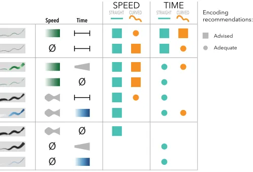
LENGTH.Encoding recommendations: SPEED
Advised
Adequate TIME
Ø
Ø
Ø
Ø
Ø
CURVED CURVED STRAIGHT STRAIGHT
[image:9.612.309.558.48.217.2]Time Speed
Fig. 12. Summary of our recommendations for encoding time and speed on 2D+time trajectories, according to the shape of the path and the information to convey.
One noteworthy result is that
S
VALUET
is not good at conveying time.This confirms our hypothesis that discriminating small variations in color value is difficult. It is worth noting that the TIMEtask, where this result occurs, asks for participants to find specific non-extremum values along an increasing gradient. In that sense, it is different from the SPEEDtask which asks only for a maximum or minimum value on a path. The nature of the tasks may explain why the value encoding is much worse for TIMEthan SPEED, but the properties of the data (time monotonically increases while speed can go up and down) encourage different tasks. Despite our findings, the literature is full of examples where time is mapped to value (e.g., [9,23,77]). In contrast, SIZE
S
T
, whichleads to more accurate perception of time than
S
VALUET
, is almost neverused for encoding time on 2D paths. Interestingly, participants were the fastest with
S
ØS
VALUET
, while making large errors. One explanationis that participants gave up and rapidly gave a best guess once they had realized that reading time is difficult with this encoding.
It is also important to note that while participants made small er-rors with
S
VALUET
LENGTH andS
ØT
LENGTH, their completion times with these encodings were slightly higher than with some other encodings. While the result are not definite and the differences are small, it raises questions about how humans decodeT
LENGTH. We can safely assume that comparing multiple segment sizes requires more effort than e.g. finding the darkest color value withS
VALUE. This is particularly true for CURVED, where segments get distorted and become harder to compare as they can have varying curvatures.Participants (see Figure 11) scored high two encodings with
T
LENGTH:VALUE
S
T
LENGTH andS
ØT
LENGTH. As for SPEED,S
SIZET
LENGTH got low scores. Interestingly, they slightly preferredS
ØT
LENGTH overVALUE
S
T
LENGTH, while it resulted in slightly larger errors for CURVED; this may be because addingS
VALUEon top ofT
LENGTHadds visual clutter.5.3 Recommendations
Most of the differences between encodings are small. However, they are consistent across TASKand SHAPE. Participants’ subjective judge-ments broadly align with quantitative findings. They found encodings with
T
LENGTHto be very good at conveying both time and speed, with the exception ofS
SIZET
LENGTH. They also foundS
VALUET
to be bad at conveyingtime. While the subjective preferences are consistent across participants for SPEED, they are less clear for TIME, as no encoding unanimously received positive judgement despite some clear differences in terms of error measure. This suggests that people may be less conscious of the efficacy of encodings when estimating time than when estimating speed. This may also be due to the fact that for the SPEEDtask, partici-pants were always looking for an extremum value, while for the TIME
To best encode speed only:
RS1 We advise encoding speed withvalue
S
VALUE. If value cannot beused (e.g., color is already used extensively), we advise conveying speed by mapping time tosegment length
T
LENGTH.RS2 If a visualization containsstraightpaths only and the important
information to convey isspeed, then any speed encoding (and LENGTH
T
) can be used. If it containscurvedpaths, we discourageencoding speed withsize
S
SIZE.To best encode time only:
RT1 We advise encoding time withsegment length
T
LENGTH, in the formof time ticks.
RT2 We discourage encoding time with value
S
VALUET
. To best encode both time and speed simultaneously:RTS1 We advise usingsegment length
T
LENGTHwhenever possible toconvey both time and speed. Encoding speed with value
S
VALUEon top of
T
LENGTHcan improve perceiving time, but may slightly interfere with perceiving speed.RTS2 If the number of available variables is limited, we advise using
segment lengthalone
S
ØT
LENGTH as this encoding conveys bothtime and speed.
RTS3 If using segment length
T
LENGTHis not possible or not desirable within the context of a visualization, we advise encoding speedwithvalueand time withsize
S
VALUE SIZES
T
.Our results are consistent with geography guidelines [49] and urban planning and traffic maps [36]. They provide quantifiable evidence that confirms existing empirical knowledge, such as that size should not be used to encode time. Also, although we do not explicitly rank the visual variables, our results are consistent with Mackinlay’s ranking of visual variables [55]. One difference is that because our results are not the same for straight and curved paths, we expect this ranking to change according to both the shape of the 2D path and the time distribution of more complex 2D+time trajectories.
5.4 Limitations and Future Work
This first empirical evaluation of visual encodings of time and speed on 2D+time trajectories allowed us to draw recommendations regarding which encoding to use for conveying time and speed independently or in combination. More than providing Infovis designers with a set of clear rules, these results open the door to a wealth of opportunities for running new studies and developing a fuller understanding of the challenges of encoding temporal data on 2D paths.
As for any perceptual study, our results and recommendations are valid within the scope of the study. In particular, we favored the diversity of encodings at the expense of constraining other factors. Our findings apply to simple shapes and value estimation tasks. However, like other focused controlled studies, our results provide precision rather than generalizability [57] and may not generalize to more complex tasks and path shapes. Perhaps the most generalizable results are those where encodings poorly conveyed either time or speed; if these encodings fail for simple tasks and paths, they should also fail for more complex tasks and path shapes. Specifically, building on our results, future studies can discard
S
VALUET
and SIZES
T
for encoding time and avoidS
SIZEfor encoding speed. We think the following factors are worth studying in the future.The pathof a 2D trajectory can be complex in many ways. We
tested path curvature, finding different results for straight and curved paths. Other path characteristics that could affect the accuracy of encodings include path direction, length, angles, and crossings:
Path Direction.While the paths in our study all started from the left and ended on the right, this is unlikely to be the case in a real-world context. Representing the direction of a 2D+time trajectory is often important (e.g., in connected scatterplots [40] and for eye-tracking scan-paths [35]), and related work indicates that humans have a leftward bias of attention [29]. This makes direction worth studying in the context of 2D+time trajectories. One could also study how time encodings provide direction on complicated paths. For example, SIZE
S
T
andS
VALUET
provide direction, while
T
LENGTHdoes not. To convey direction when mapping time toT
LENGTH, one could also map time toS
VALUET
, althoughVALUE
S SVALUE
VALUE
T
SIZE
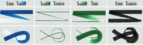
[image:10.612.325.559.51.126.2]S TLENGTH TSIZE SSIZE TLENGTH
Fig. 13. Some encodings for paths with sharp corners and loops.
this would prevent using
S
VALUEto encode speed. An alternative is to mark time ticks with arrowheads instead of perpendicular lines.Path Length.We tested paths with similar lengths. Further studies could assess the effect of path length on the perception of encodings. We envision that encodings which show the absolute value of time at each point along the path in a continuous manner (SIZE
S
T
andS
VALUET
) willlead to larger errors as the length of the path increases, as this puts further stress on our ability to perceive small variations. One could increase the maximum size of the path with SIZE
S
T
, but this would clutter the visualization. In contrast, we expectT
LENGTH– which scales well since it shows relative time – to be robust to longer paths.Path Angles.Our paths had smooth angles. While this can be the case (e.g., Figures 2 and 7), paths often have sharp corners, e.g., road trips can feature 90 degree turns. Sharp corners encoded with
S
SIZEorSIZE
S
T
may be less useful due to visual artifacts and overlaps (Figure 13). Path crossings. We tested individual paths that do not cross. The perception of encodings will be affected if one or more paths cross (see Figure 13). For example,S
VALUEandS
VALUET
will be difficult to read when they overlap.S
SIZEand SIZES
T
suffer from the same problem if theencoding is fully opaque, but transparency may improve the result. We expect
T
LENGTHto be more robust for paths that cross.The contextsurrounding a 2D+time trajectory plays an important
role in the perception of graphical encodings. We used a light gray background so that color ramps can contain white. In many cases, mapping time or speed to color will not be an option if surrounding elements already make use of a variety of colors. To a lesser extent, the context can affect
T
LENGTH. For example, latitude lines on a map (see Figure 7) or contour lines on a contour map would conflict with time ticks and make it more difficult to decode time and speed. Also,S
SIZEand SIZE
S
T
are likely to impact the surroundings because they take much screen real estate. Finally, when objects are represented on 2D+time trajectories, such as players on a soccer field [60], fixation times on eye-tracking scanpaths [35], or the data points in Figure 4, the manner of their representation may constrain which encoding can be used.The time functionof a 2D+time trajectory can affect the perception
of encodings. In this study, we used a variety of time functions. Future work could study the differences between various time distributions and ranges of speeds. Some encodings may be better for small and smooth variations, some for large and abrupt variations, and others may be more robust to the whole spectrum of possible distributions.
6 CONCLUSIONS
Results of our graphical perception study of nine visual encodings provide advice for encoding time and speed on simple 2D+time trajec-tories. However, it is important to remember that 2D+time trajectories are more general than spatio-temporal trajectories. Our findings ap-ply not only to spatial data, but also to abstract representations that need to convey speed and/or time but already make use of the two dimensions of the plane. This is the case for example with connected scatterplots [40], eye-tracking data [14] and other time-evolving ab-stract data graphics [46]. We hope that these initial results will help researchers design new studies to develop a fuller understanding of how to best visually encode 2D+time trajectories.
7 ACKNOWLEDGMENTS
REFERENCES
[1] W. Aigner, S. Miksch, H. Schumann, and C. Tominski.Visualization of time-oriented data. Springer, Berlin, Germany, 2011.
[2] R. Amar, J. Eagan, and J. Stasko. Low-level components of analytic activity in information visualization. InProc. INFOVIS ’05, pp. 15–. IEEE Computer Society, Washington, DC, USA, 2005. doi: 10.1109/INFOVIS. 2005.24
[3] American Psychological Association. The Publication manual of the American psychological association. American Psychological Association Washington, Washington, DC, 6th ed., 2013.
[4] F. Amini, S. Rufiange, Z. Hossain, Q. Ventura, P. Irani, and M. J. McGuffin. The impact of interactivity on comprehending 2d and 3d visualizations of movement data. IEEE Transactions on Visualization and Computer Graphics, 21(1):122–135, Jan 2015. doi: 10.1109/TVCG.2014.2329308 [5] G. Andrienko, N. Andrienko, and S. Wrobel. Visual analytics tools for analysis of movement data.SIGKDD Explor. Newsl., 9(2):38–46, Dec. 2007. doi: 10.1145/1345448.1345455
[6] N. Andrienko and G. Andrienko. Exploratory Analysis of Spatial and Temporal Data: A Systematic Approach. Springer-Verlag New York, Inc., Sankt Augustin, Germany, 2005.
[7] N. Andrienko and G. Andrienko. Visual analytics of movement: An overview of methods, tools and procedures. Information Visualization, 12(1):3–24, 2012.
[8] B. Bach, P. Dragicevic, D. Archambault, C. Hurter, and C. Sheelagh. A review of temporal data visualizations based on space-time cube opera-tions. InEurographics Conference on Visualization. Eurographics, IEEE, Swansea, Wales, UK, 2014.
[9] B. Bach, C. Shi, N. Heulot, T. Madhyastha, T. Grabowski, and P. Dragice-vic. Time curves: Folding time to visualize patterns of temporal evolution in data. IEEE Transactions on Visualization and Computer Graphics, 22(1):559–568, Jan 2016. doi: 10.1109/TVCG.2015.2467851
[10] J. Bertin.Semiology of Graphics. University of Wisconsin Press, Wiscon-sin, US, 1983.
[11] A. Bezerianos and P. Isenberg. Perception of visual variables on tiled wall-sized displays for information visualization applications.IEEE Transac-tions on Visualization and Computer Graphics, 18(12):2516–2525, 2012. [12] H. Bhatia, S. Jadhav, P. T. Bremer, G. Chen, J. A. Levine, L. G. Nonato, and V. Pascucci. Flow visualization with quantified spatial and temporal errors using edge maps.IEEE Transactions on Visualization and Computer Graphics, 18(9):1383–1396, Sept 2012. doi: 10.1109/TVCG.2011.265 [13] S. Bies and M. Van Kreveld. Time-space maps from triangulations. In
International Symposium on Graph Drawing, pp. 511–516. Springer, Springer, Berlin, Heidelberg, 2012.
[14] T. Blascheck, K. Kurzhals, M. Raschke, M. Burch, D. Weiskopf, and T. Ertl. State-of-the-Art of Visualization for Eye Tracking Data. In R. Borgo, R. Maciejewski, and I. Viola, eds.,EuroVis - STARs. The Eurographics Association, 2014. doi: 10.2312/eurovisstar.20141173 [15] N. Boukhelifa, A. Bezerianos, T. Isenberg, and J. D. Fekete. Evaluating
sketchiness as a visual variable for the depiction of qualitative uncertainty.
IEEE Transactions on Visualization and Computer Graphics, 18(12):2769– 2778, Dec 2012. doi: 10.1109/TVCG.2012.220
[16] K. Buchin, A. van Goethem, M. Hoffmann, M. J. van Kreveld, and B. Speckmann. Travel-time maps: Linear cartograms with fixed ver-tex locations. InProc. GIScience, pp. 18–33. Springer, Berlin, Heidelberg, 2014. doi: 10.1007/978-3-319-11593-1 2
[17] F. Chevalier, P. Dragicevic, and S. Franconeri. The not-so-staggering effect of staggered animated transitions on visual tracking.IEEE Transactions on Visualization and Computer Graphics, 20(12):2241–2250, Dec 2014. doi: 10.1109/TVCG.2014.2346424
[18] L. Chittaro, R. Ranon, and L. Ieronutti. Vu-flow: A visualization tool for analyzing navigation in virtual environments.IEEE Transactions on Visualization and Computer Graphics, 12(6):1475–1485, Nov 2006. [19] W. Cleveland and R. McGill. Graphical Perception and Graphical Methods
for Analyzing Scientific Data.Science, 229(4716):828, 1985.
[20] W. S. Cleveland and R. McGill. Graphical perception: Theory, experimen-tation, and application to the development of graphical methods.Journal of the American statistical association, 79(387):531–554, 1984. [21] W. S. Cleveland and R. McGill. An experiment in graphical perception.
International Journal of Man-Machine Studies, 25(5):491–500, 1986. [22] W. S. Cleveland and R. McGill. Graphical perception: The visual decoding
of quantitative information on graphical displays of data.Journal of the Royal Statistical Society. Series A (General), 150(3):192–229, 1987. [23] C. Collberg, S. Kobourov, J. Nagra, J. Pitts, and K. Wampler. A system for
graph-based visualization of the evolution of software. InProc. SoftVis, pp. 77–ff. ACM, New York, NY, USA, 2003. doi: 10.1145/774833.774844 [24] M. Correll and M. Gleicher. Error bars considered harmful: Exploring
alternate encodings for mean and error. IEEE Transactions on Visual-ization and Computer Graphics, 20(12):2142–2151, Dec 2014. doi: 10. 1109/TVCG.2014.2346298
[25] D. Cousineau. Confidence intervals in within-subject designs: A simpler solution to loftus and massons method.Tutorial in Quantitative Methods for Psychology, 1(1):42–45, 2005.
[26] F. E. Croxton and H. Stein. Graphic comparisons by bars, squares, circles, and cubes.Journal of the American Statistical Association, 27(177):54–60, 1932.
[27] F. E. Croxton and R. E. Stryker. Bar charts versus circle diagrams.Journal of the American Statistical Association, 22(160):473–482, 1927. [28] G. Cumming and S. Finch. Inference by eye: Confidence intervals and
how to read pictures of data.American Psychologist, 60(2):170, 2005. [29] C. A. Dickinson and H. Intraub. Spatial asymmetries in viewing and
remembering scenes: Consequences of an attentional bias? Attention, Perception, & Psychophysics, 71(6):1251–1262, 2009. doi: 10.3758/APP. 71.6.1251
[30] E. Dimara, A. Bezerianos, and P. Dragicevic. The attraction effect in infor-mation visualization.IEEE Transactions on Visualization and Computer Graphics, PP(99):1–1, 2016. doi: 10.1109/TVCG.2016.2598594 [31] P. Dragicevic. Fair statistical communication in hci. InModern Statistical
Methods for HCI, pp. 291–330. Springer, Berlin, Heidelberg, 2016. [32] J. Dykes and D. Mountain. Seeking structure in records of spatio-temporal
behaviour: visualization issues, efforts and applications.Computational Statistics & Data Analysis, 43(4):581 – 603, 2003. Data Visualization. doi: 10.1016/S0167-9473(02)00294-3
[33] W. C. Eells. The relative merits of circles and bars for representing compo-nent parts.Journal of the American Statistical Association, 21(154):119– 132, 1926.
[34] P. Gatalsky, N. Andrienko, and G. Andrienko. Interactive analysis of event data using space-time cube. InProc. IV, pp. 145–152. IEEE, London, UK, July 2004. doi: 10.1109/IV.2004.1320137
[35] J. H. Goldberg and J. I. Helfman. Visual scanpath representation. In
Proceedings of the 2010 Symposium on Eye-Tracking Research & Applications, ETRA ’10, pp. 203–210. ACM, New York, NY, USA, 2010. doi: 10.1145/1743666.1743717
[36] K. P. Goldsberry. Real-time traffic maps.
[37] T. Gschwandtner, M. Bogl, P. Federico, and S. Miksch. Visual encodings of temporal uncertainty: A comparative user study.IEEE Transactions on Visualization and Computer Graphics, 22(1):539–548, 2016.
[38] T. H¨agerstrand. Wath about people in regional science? Regional Science Association, 24:7–21, 1970.
[39] M. Hancock, M. Nacenta, C. Gutwin, and S. Carpendale. The effects of changing projection geometry on the interpretation of 3d orientation on tabletops. InProc. ITS ’09, pp. 157–164. ACM, New York, NY, USA, 2009. doi: 10.1145/1731903.1731934
[40] S. Haroz, R. Kosara, and S. L. Franconeri. The connected scatterplot for presenting paired time series. IEEE Transactions on Visualization and Computer Graphics, 22(9):2174–2186, Sept 2016. doi: 10.1109/TVCG. 2015.2502587
[41] Y. Jansen and K. Hornbaek. A psychophysical investigation of size as a physical variable.IEEE Transactions on Visualization and Computer Graphics, 22(1):479–488, Jan 2016. doi: 10.1109/TVCG.2015.2467951 [42] Y. Jansen and K. Hornbæk. A psychophysical investigation of size as a physical variable.IEEE Transactions on Visualization and Computer Graphics, 22(1):479–488, 2016.
[43] C. Kaiser, F. Walsh, C. J. Farmer, and A. Pozdnoukhov. User-centric time-distance representation of road networks. InInternational Conference on Geographic Information Science, pp. 85–99. Springer, Springer Verlag, Berlin, Heidelberg, 2010.
[44] T. Kapler, R. Eccles, R. Harper, and W. Wright. Configurable spaces: Temporal analysis in diagrammatic contexts. InProc. VAST, pp. 43–50. IEEE Computer Society, Red Hook, NY, USA, Oct 2008. doi: 10.1109/ VAST.2008.4677355
[45] K. N. Kirby and D. Gerlanc. BootES: An r package for bootstrap confi-dence intervals on effect sizes.Behavior research methods, 45(4):905–927, 2013.
![Fig. 2. Minard’s comparison of Hannibal’s second Punic war campaign(top) and Napoleon’s Russian campaign (bottom) [58].](https://thumb-us.123doks.com/thumbv2/123dok_us/1426043.95257/3.612.313.551.48.255/minard-comparison-hannibal-second-campaign-napoleon-russian-campaign.webp)