A comparative study of discrete velocity methods for low-speed rarefied gas flows

(1)

Contents lists available at ScienceDirect

Computers

and

Fluids

journal homepage: www.elsevier.com/locate/compfluid

A

comparative

study

of

discrete

velocity

methods

for

low-speed

rareﬁed

gas

ﬂows

Peng Wang

a

_{, Minh Tuan Ho}

a

_{, Lei Wu}

a

_{, Zhaoli Guo}

b

_{, Yonghao Zhang}

a,∗

a_James_Weir_Fluids_Laboratory,_Department_of_Mechanical_and_Aerospace_Engineering,_University_of_Strathclyde,_Glasgow_G1_1XJ,_UK b_State_Key_Laboratory_of_Coal_Combustion,_Huazhong_University_of_Science_and_Technology,_Wuhan_430074,_China

a

r

t

i

c

l

e

i

n

f

o

Articlehistory: Received8July2017 Revised26October2017 Accepted12November2017 Availableonline13November2017

Keywords: Gaskineticequation Rareﬁedﬂow

Discretevelocitymethod Discreteuniﬁedgaskineticscheme

a

b

s

t

r

a

c

t

Inthestudy ofrarefiedgasdynamics,thediscrete velocitymethod(DVM) hasbeenwidelyemployed tosolvethegaskineticequations.AlthoughvariousversionsofDVMhavebeendeveloped,their perfor-mance,intermsofmodelingaccuracyandcomputationalefficiency,isyettobecomprehensivelystudied inalltheflowregimes.Here, thetraditionalthird-ordertime-implicitGodunovDVM(GDVM)and the recentlydevelopeddiscreteunifiedgas-kineticscheme(DUGKS)areanalysedinfindingsteady-state so-lutionsofthelow-speedforce-drivenPoiseuilleandlid-drivencavityflows.Withthemolecularcollision andfreestreamingbeingtreatedsimultaneously,theDUGKSpreservesthesecond-orderaccuracyinthe spatialandtemporaldiscretizationsinallflowregimes.Towardsthehydrodynamicflowregime,notonly istheDUGKSfasterthantheGDVMwhenusingthesamespatialmesh,butalsorequireslessspatial res-olutionthanthatoftheGDVMtoachievethesamenumericalaccuracy.Fromthesliptofreemolecular flowregimes,however,theDUGKSisslowerthantheGDVM,duetothecomplicatedfluxevaluationand therestrictivetimestepwhichissmallerthanthemaximumeffectivetimestepoftheGDVM. There-fore,theDUGKSispreferable forproblemsinvolvingdifferentflowregimes,particularlywhenthe hy-drodynamicflowregimeisdominant.Forhighlyrarefiedgasflows,ifthesteady-statesolutionismainly concerned,theimplicitGDVM,whichcanboosttheconvergencesignificantly,isabetterchoice.

1. Introduction

Multi-scale flows, wheredifferent temporal and spatial scales are presented, are often found in nature and engineering, which represent a modeling and simulation challenge. The gas flow at different scales can be categorizedby the Knudsen number(Kn), defined as the ratio of the mean free path of gas molecules to thecharacteristiclengthoftheflowfield.Itiswellrecognizedthat thecomputationalfluiddynamicsbasedontheNavier-Stokes(NS) equations andthedirect simulationMonte Carlo (DSMC)method [1]aretwo dominantmethods fortheefficientandaccurate sim-ulation of the hydrodynamic (Kn_<10−3 ) and rarefied gas (tran-sition, 0.1<Kn<10; free molecular, Kn>10) flows, respectively. However, intheslipregime(10−3 <Kn<0.1),theNS solversand theDSMCmethodbecome eitherinaccurate orinefficient:theNS equationsareinappropriate todescriberarefied(non-equilibrium) gas flows because they are derived basedupon the near equilib-rium hypothesis, while the particle nature of the DSMC method

∗ _{Corresponding}_author.

E-mailaddress:[email protected](Y.Zhang).

restricts its application in near hydrodynamic regime [2], as the temporalandspatialresolutionsmustbesmallerthanthe molec-ularcollisiontime andmeanfreepath,respectively.Therefore,for multi-scalegasflows,itisintuitive tousecontinuum-particle hy-bridmethodsthatsolvetheflowfieldsindifferentregimesby ap-propriate solvers [3–6]. However, hybridmethods may encounter great difficulties forflows with a continuousand complex varia-tionofflowphysics[7].

TheBoltzmannequationisafundamentalmodelfordilutegas flows in all the flow regimes, which uses single-particle veloc-itydistribution functiondefinedinasix-dimensionalphasespace todescribe the systemstate. Near the hydrodynamicregime, the NS equations can be derived through the Chapman–Enskog ex-pansion.However, thenumericalsolutionoftheBoltzmann equa-tion remains a research challenge. In the past two decades, de-terministicnumerical methods have beendeveloped to solve the Boltzmannequation [8],mostofwhich arebased onthediscrete velocity method (DVM) [9–13] that approximates the continuous molecularvelocityspacebydiscretevelocitypoints,sothatthe re-sultingequationscan besolvednumerically[10].Manyfull Boltz-mannsolvers [14–19],especiallythefastspectralmethod[19–21],

https://doi.org/10.1016/j.compﬂuid.2017.11.006

(2)

provideaccurate numerical results,which canserve asthe refer-encesolutions. However, thehighcomputational cost in calculat-ingthecomplicatedcollisionoperatormakesthemimpracticalfor manyapplications[8]. Therefore,the Boltzmannequation is usu-ally replaced by simpliﬁed kinetic model equations, such asthe Bhatnagar–Gross–Krook(BGK)[22],ellipsoidalstatistical(ES)[23], andShakhov [24] models. And most of DVMsare developed for theseBoltzmannmodelequations.

In the traditional DVM, the Boltzmannmodel equation is ex-plicitlysolved through the operator splitting method[15], where thetime stepandcellsizeare limitedbythemeancollisiontime andmean free path ofgas molecules,respectively. Consequently, liketheDSMCmethod,theDVMworkswellforhighlyrarefiedgas flows, but encounters great difficulties for near-continuum flows [25,26].Some semi-implicit andimplicit DVMshave been devel-opedto remove therestriction ofthe time stepandimprove the efficiency[10,27,28].

In orderto develop an efficientDVM forall theflow regimes, significant efforthas been made recently to develop the asymp-toticpreserving(AP) schemes[11,27–31].An APmethodis stable withrespecttoKn,andwhenKnisverysmall,itisconsistentwith theChapman-Enskogrepresentationinthecontinuumlimit[8,31]. Therefore,theAPpropertyiscriticaltoamulti-scalemethod. Un-fortunately,mostAPschemescanonlyrecovertheEulersolutions inthehydrodynamiclimit,exceptfortherecentlydeveloped uni-fiedgas-kineticscheme(UGKS)[25,26,31–33]andthediscrete uni-fied gas-kinetic scheme (DUGKS) [34–39], which recover the NS solutions. Boththe UGKS and DUGKSshare the same merit that themoleculartransportprocessiscoupledwiththemolecular col-lision,sothatthetimestepandmeshsizeareindependentofthe collisiontimeandthemeanfreepath,respectively[25].

The maindifferencebetweentheUGKSandDUGKSliesinthe constructionof thedistributionfunction across thecell interface: theUGKSusesthelocalintegrationsolutionofthekinetic model, whiletheDUGKSadoptsitsdiscretecharacteristicsolution,thereby avoidscomputing thecomplicated gradients ofmacroscopic vari-ables. Also, owing to auxiliary functions introduced, the DUGKS onlyupdatessingledistributionfunctionintheevolutionprocess, whileintheUGKSmacroscopicvariablesanddistributionfunction areupdatedwithin onetime step.Therefore,theDUGKSisbetter than the UGKS in terms of simplicity and eﬃciency, while their accuraciesareatthesamelevel[40,41].

So far, the DVM can be roughly classifiedinto two types: the traditional DVM and new AP DVM. The detailed comparison of thesetwomethods willprovideessentialinformationforusersto choosetheappropriateone forapplications.Inthispaper,wewill perform a comparative study ofthese two type DVMsin all the flowregimes,aimingtoclarifytheirapplicabilityfordifferentflow problems.Itisusuallyrecognizedthat itisnoteasy fora second-order accurate traditional DVM to simulate the continuum flow dueto thelimitationsofmeshsize andtime step,hencea third-orderaccuratetime-implicitGodunovDVM(GDVM)[10]isadopted hereinall the flow regimes includingthe hydrodynamicregime. Ontheother hand,it hasbeendemonstratedthat theDUGKS,as anewly developedAPDVM,candynamically describeflows from the free molecular to hydrodynamic regimesand simultaneously preservea second-order accuracy inboth the spatialand tempo-ralspaces[36,40,42].Althoughthetwomethodsare derivedfrom thesamemodelequation,differentalgorithmswillleadtosolution discrepancy.Inthiswork,wewillanalyzethesetwotypicalDVMs intermsofaccuracyandefficiency.

The remaining part of this paperis organized as follows.We ﬁrst make a brief introduction of the time-implicit GDVM and DUGKS, as well as an analysis of both methods in Section 2. The detailed comparison of these two methods regarding

accu-racy andeﬃciencyisgiven inSection 3,followed by conclusions inSection4.

2. Numericalmethods

In this section, the GDVM [10] and DUGKS [35] are used to solvetheShakhovmodelequationformonatomicgases[24].

2.1. TheShakhovmodel

In the absence of external force, the Shakhov kinetic model equationcanbewrittenas

∂

f

∂

t +

ξ

·

∇

f=−

1

τ

f−fS

_, ₍₁₎

where f₌ f

(

x_,

ξ

_,t

)

is the velocity distribution function of gas molecules with the molecular velocity

ξ

=

(

c2 RT −5

)

= feq₊_f

Pr, (2)

wherePristhePrandtl number,c₌

ξ

₋U isthepeculiarvelocity withUbeingthemacroscopicﬂowvelocity, q= 1

2 cc2 fd

ξ

isthe heatﬂux, Risthe speciﬁcgasconstant, andT isthetemperature ofthegas.Thecollisiontime

τ

inEq.(1)isrelatedtothedynamic viscosity

μ

andpressurepby

τ

=

μ/

p.The Maxwellian distribu-tionfunctionfeq_is_given_by

feq₌

ρ

(

ρ

E)T_are_calculated_from thevelocitymomentsofthedistributionfunction:

W =

ψ

fd

ξ

, (4)

where

ψ

=

1,

ξ

,1 2

ξ

2

T

and

ρ

E= 1

2

ρ

2 _g₊_h

₎

_d

_ξ

_,

q= 1 2 c

(

c

2 _g₊_h

₎

_d

_ξ

_. ₍₆₎

Thegoverningequationsforthetworeduceddistribution func-tionscanbededucedfromEq.(1)as

∂

g

∂

t +

ξ

·

∇

g=

g=−

1

τ

g−gS

_, _(7a)

∂

h

∂

t +

ξ

·

∇

h=

h=−

1

τ

(3)

wherethereducedreferencedistributionfunctionsgS _and_hS_are

2

π

RT exp

− c2

2RT

, (9a)

heq=RTgeq, (9b)

gPr =

(

1−Pr

)

₅c_pRT·q

c2 RT −4

geq, (9c)

hPr =

(

1−Pr

)

₅c_pRT·q

c2 RT −2

heq. (9d)

ItisclearthattheupdatingrulesforgandhinEq.(8)havethe samestructure

∂φ

∂

t +

ξ

·

∇

φ

=

=−

1

τ

φ

−

φ

S

, (10) wherethegenericsymbol

φ

isusedtodenotegorh.

Notethat thedynamicviscosity

μ

λ

ref as

λre f

=

μre f

p

π

RTre f

2 . (12)

UsingtheKnudsennumber(Kn),Machnumber(Ma)andReynolds number(Re),whicharerespectivelydeﬁnedas

Kn=

λre f

Lre f

, Ma= Ure f

γ

RTre f

, Re=

ρre f

Ure fLre f

μre f

, (13)

andtheyarerelatedby

Kn=

πγ

2

Ma

Re, (14)

where

γ

isthespeciﬁcheat ratio,L_ref,U_ref and

ρ

_ref are the refer-encelength,velocityanddensity,respectively.

2.2. Thetraditionaldiscretevelocitymethod

The traditional DVM we adopt here is also based on Eq. (10) which is discretized in time by the fully time-implicit Godunov-typescheme[10,43]:

₁

tn +

ξ

·

∇

+ 1

τ

n

j =

⎧

⎨

⎩

2 φn j+1+3 φ

n j−6 φ

n j−1+φ

n j−2

6x ,

ξ

x > 0 −2 φn

j−1−3 φnj+6 φnj+1−φnj+2

can besmallerthan 1tocapturethetransient behavior, it can also be set aslarge as 104 for steady-state ﬂow problems.

2.3.Discreteuniﬁedgas-kineticscheme

The DUGKS is an explicit ﬁnite-volume method to solve Eq.(10).Thecomputationaldomainisﬁrstdividedintosome con-trol cells; then integrating Eq. (10) in a cell Vj (centered at xj) from time tn to tn+1

(

t=tn+1 −tn

)

, and using the trapezoidal andmiddle-pointrulesforthetimeintegrationofthecollisionand convectionterms,respectively,we canobtain theevolution equa-tionofDUGKS:

˜

φ

n+1

j =

φ

˜+, n j −

t

|

Vj

|

F

n+1/2

j , (17)

where

˜

φ

=

φ

−

t 2

=

2

τ

+

t

2

τ φ

−

t

τ

+

t

φ

˜+

2

t

2

τ

+

t

φ

S_, _(18b)

aretwoauxiliarydistributionfunctions,and

Fn+1 /2 ₌

ξ

2

g+

h

)

d

ξ

=0,we can

E=1₂

(

ξ

2 _g_˜₊_h˜

₎

_d

_ξ

_, ₍₂₀₎

andtheheatﬂuxfrom

q= 2

τ

2

τ

+

˜ istoevaluatethe micro-ﬂux F, which is solely determined by the gas distribution function

φ

n+1 /2

₍

_x

f,

ξ

)

on the cell interface xf and at the half time step

tn+1 /2 . To do so, in the DUGKS, Eq. (10) is integrated along the characteristiclinewithinahalftimesteps=

t/2,

φ

n+1 /2

₍

_x

f,

ξ

)

−

φ

n

(

xf−

ξ

s,

ξ

)

= s

2

n+1 /2

₍

_x

f,

ξ

)

+

n

(

xf−

ξ

s,

ξ

)

(4)

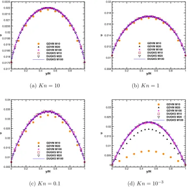
Fig.1. Thevelocityproﬁles(normalizedbyξ0)alongthechannelcross-sectionat(a)Kn=10,G=0.01(b)Kn=1,G=0.01(c)Kn=0.1,G=0.01and(d)Kn=10−3,

G=10−4_obtained_from_the_DUGKS_and_GDVM_simulations_with_different_spatial_{discretizations.}_M10,_M20_and_M100_represent_the_results_with_10,₂₀_and₁₀₀_grid_points

alongthechannelcrosssection,respectively.Thesamenotationsarealsousedinthefollowingﬁgures.

wheretime integration of the collision term is approximated by the trapezoidal rule. Again, in order to remove the implicity of Eq.(22),twodistributionfunctionsareintroduced

¯

φ

=

φ

− s 2

=

2

τ

+s

2

τ φ

−

s

2

τ φ

S_, _(23a)

¯

φ

+₌

_φ

₊ s 2

=

2

τ

−s

2

τ

+s

φ

¯−

2s

2

τ

+s

φ

S_. _(23b)

ThenEq.(22)isexpressedexplicitlyas ¯

φ

n+1 /2

₍

_x

f,

ξ

)

=

φ

¯+,n

(

xf−

ξ

s,

ξ

)

, (24)

where

φ

¯+,n_is_constructed_as

¯

φ

+,n

₍

_x

f−

ξ

s,

ξ

)

=

φ

¯+,n

(

xj,

ξ

)

+

(

xf−xj−

ξ

s

)

·

σ

j,

(

xf−

ξ

s

)

∈Vj, (25)

_x f,

ξ

)

=

2

+s

φ

S,n+1 /2

₍

_x f,

ξ

)

,

(26)

where

φ

S,n+1 /2

₍

_x

b,

ξ

)

isdeterminedbytheconservedvariablesand the heat ﬂux on the cell interface xb and at the half time step

E=1 2

(

ξ

2 _g_¯₊_h¯

₎

_d

_ξ

_, ₍₂₇₎

and

q= 2

τ

2

τ

+sPrq¯, withq¯= 1 2 c

(

c

2 _g_¯₊_h¯

₎

_d

_ξ

_. ₍₂₈₎

Thenthemicro-ﬂuxcanbecomputedbyEq.(26).Finally

φ

˜ atthe cellcentercanbeupdatedaccordingtoEq.(17).Notethatthetime stepintheDUGKSissolelydeterminedbytheCFLcondition.

BoththeGDVMandDUGKSpresentedabovearebasedon con-tinuousvelocity spaceforconvenience. Inactual implementation, the continuous velocity spaceis discretized into a ﬁnite discrete velocity set {

ξ

i} the same as that of the traditional DVM [10]. For example,in the DUGKS,the distribution functionsi.e., g˜and ˜

h are approximated at these discrete velocity points as g˜i and ˜

hi. Properquadraturerule, such asthe Newton-Cotesand Gauss-Hermitequadratures,areadoptedtoapproximatethemoments,

ρ

= i

ig˜i,

ρ

U=

i

ξ

ig˜i,

ρ

E= 1 2

i

ξ

2

ig˜i+h˜i

,

[image:4.595.109.483.56.425.2]

(5)

Fig.2. Apparentgaspermeability(normalizedbyGH2₎_in_the_Poiseuille_ﬂow_at_different_Kn_:₍_a₎_0.1_≤_Kn_≤_10,₍_b₎₁₀−4_≤_Kn_≤₀_.₁_.

whereϖi istheweightcoeﬃcientsforthecorresponding quadra-turerule.

2.4. AnalysisoftheDUGKSandGDVM

Boththe DUGKSandGDVMare derivedfrom thesame Boltz-mann model equation, butdifferent considerations in their algo-rithmsdeterminetheirdistinctivebehaviorsinﬂowsimulations.

Inthe DUGKS,theﬂux issolelydetermined by molecular dis-tributionfunctionsacrossthecellinterfaces,whichisconstructed onbasisofthediscretecharacteristicsolutionofthekineticmodel. BasedonEqs.(23),(24)and(26),itcanberewrittenas

φ

n+1 /2

₍

_x f,

ξ

)

=

2

τ

2

τ

+s

φ

¯+,

n

₍

_x

f−

ξ

s,

ξ

)

+

s

2

tiscomparableto

τ

,therebyboththekineticand hydrody-namicphysicsareimportant.Therefore,withvariationoftheratio of

t/

τ

, the DUGKS can dynamically describe the ﬂow fromthe freemolecular tohydrodynamicregimes.It alsohasbeen demon-strated that with the coupled treatment of molecular transport andcollision processes,the numericaldissipation in DUGKSis at

O

(

x2

)

+O

(

t2

)

[38].

Incontrast,intheGDVM,themodelequationisdirectlysolved using the implicit finite-difference method, and the convection term is approximated by the upwindscheme, which means that molecules transport across two grid points freely. Therefore, for flow regimesin which mesh size is much larger than the mean free path, the use of upwind scheme is obviously inappropriate, since molecules will physically encounter many collisions when theytransportsuchalongdistanceinameshsizescale.Thus,the GDVM requiresmuch finer mesh to resolvethe flow in the near continuumregimes[26].Notethattheadoptionofthethird-order upwindapproximationEq.(16)fortheconvectionterminthe ex-plicit part of Eq. (15) may improve the GDVM’s performance in

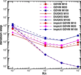
Fig.3. Iterationstepsrequiredtoreachthestead-statedeﬁnedbyEq.(33)at dif-ferentKnandmeshes.NotethattheconvergencecriteriaforimplicitGDVMis esti-matedforonetimestep.

thecontinuum andnear-continuum regimes.Itis alsonotedthat thisﬁnite-difference DVM computes lessequilibrium state distri-bution functions than the DUGKS with a ﬁnite-volume formula-tion,thus,withthesameCFLnumber,theGDVMshouldbefaster than DUGKS for each iteration. In addition, it should be bear in mindthat theGDVM becomesan implicit methodwhen usinga largerCFLnumber(

η

1), anditwill leadtofastconvergenceof theGDVM.

Therefore,the DUGKSmay work well inall the flow regimes, and the GDVM is preferable for highly rarefied flows, but may encounter great difficulty in the continuum andnear continuum regimes.Itshouldbenotedthatalthoughthetimestep

tinthese twomethodsarebothdeterminedbytheCFLcondition,forGDVM,

tisapseudo-timestepandhasnocontributiontothenumerical error,thereby the results obtainedby theGDVM with smallCFL numberandthe implicitGDVMwithlargerCFL numberhavethe sameaccuracy. Theabove pointswillbe veriﬁedinthe following simulations.

3. Numericalresultsanddiscussions

3.1. Force-drivenPoiseuilleﬂow

[image:5.595.122.488.55.232.2] [image:5.595.357.518.257.404.2]

(6)

-Fig.4. ComparisonoftheapparentgaspermeabilityofthePoiseuilleﬂowdriven byaforceandapressuregradient.Themeshpointsof20and10areappliedinthe GDVMandDUGKSsimulations,respectively,inwhichthemeshindependentresults areobtained.

direction,sothattheShakhovmodelEq.(10)becomes

∂φ

∂

t +

ξ

y

∂φ

∂

y =

+Fx, (31)

whereFxistheforceterm.Supposethemagnitudeoftheexternal accelerationGis verysmall,the force termcan be approximated

by

Fx=−G

∂φ

∂ξ

x ≈ −

G

∂φ

eq

∂ξ

x ,

(32)

where

φ

eq _is_formed_in_Eqs._(9a)_and_(9b)_.

In the GDVM, Eq.(31) is directly solved by considering Fx as a source term, while in the DUGKS, the Strang splitting method isused [44]: atthebeginning ofeach time step,the distribution function

φ

˜n _is_updated _within _a _half _time _step _by

_∂

t

φ

˜=

tFx/2, andthentheprocedureofDUGKSisexecuted followedby updat-ing

φ

˜n+1 _within_a _half _time _step_in _the_same _way_as_that _at_the beginningofeachiteration.

Inoursimulations,weuse10,20,and100uniformmeshpoints betweentwoparallelplateswiththedistanceH₌1.Thegasﬂow fromthehighlyrareﬁedto thehydrodynamicregimes(the Knud-sen number from 10 to 10−4 ) is simulated by varying the gas pressure. The diffuseboundary condition is applied on both the plates.Thehard-spheregasisconsidered,wheretheexponent

ω

in Eq.(11)is0.5.Asamatteroffact,whenthemagnitudeofexternal forceissmall,theflowisnearlyisothermal,sothatthemassflow rateis not affected by the temperature-dependence of the shear viscosity.Oursimulationsstartfromaglobalequilibriumstate.The convergencecriterionforthesteady-stateisdefinedby

t−100

t

)

|

u

(

t

)

|

< 10−

6 _. ₍₃₃₎

The discretizationof themolecular velocity space dependson the rarefaction level of the gas ﬂow. In this study, we focus on

[image:6.595.78.240.56.203.2] [image:6.595.112.476.363.730.2]

(7)

Fig.6. TheresultsofthecavityflowatKn=1:(a)U-velocityalongtheverticalcenterline,(b)V-velocityalongthehorizontalcenterline,(c)theheatfluxQxalongthe verticalcenterlineand(d)theheatfluxQyalongthehorizontalcenterline.

the low-speed flows, so for the near hydrodynamic regime, the highlyaccurateGauss–Hermiteintegrationwithfewerdiscrete ve-locity points is usually applied, while the Newton–Cotes formu-las withmore discrete velocity pointscould be adopted to cap-turediscontinuitiesin thedistribution function inhighlyrarefied regime.Therefore,forthecasesof1_≤Kn_≤10and0.1_≤Kn_<1,we, respectively, use the 100×100 and 50×50 non-uniform discrete velocity points[19]atfiniterangeof[−4,4]×[−4,4]to approxi-matethecontinuousmolecularvelocity space,whileforthecases of0.01≤Kn<0.1and10−4 ≤Kn<0.01,the28×28and8×8 half-range Gauss-Hermit discrete velocity points are applied, respec-tively.Notethatalltheparameterspresentedinthispaperare di-mensionless, wherethe spatiallength andmolecular velocity are scaledbyHand

ξ

₀=√2RTw,respectively.

ThevelocityprofilesalongthechannelcrosssectionatKn=10, 1,0.1, and10−3 are plottedinFig.1.The numerical resultsof the DUGKS withgridpoints of100 can beregarded asthe reference solutions. It is found that the DUGKS can give adequately accu-rate results with just 10 grid points in all the flows, while for the GDVM, 20 and100 mesh pointsare respectively requiredin highly rarefied and near-continuum regimes. For example, when

Kn₌10−3 _,theGDVMwith20meshpointsunderpredicts the ve-locity in the channel center by 16%, while that of the DUGKSis only2%evenwithacoarsermeshof10,seeFig.1(d).

Wethencomparetheapparentgaspermeability

κ

predictedby theGDVMandDUGKS,whichisdeﬁnedby[48]

κ

= √2Kn

π

GH2

H

0 u

(

y

)

dy. (34)

[image:7.595.119.488.55.422.2]

(8)

Fig.7. TheresultsofthecavityflowatKn=0.1:(a)U-velocityalongtheverticalcenterline,(b)V-velocityalongthehorizontalcenterline,(c)theheatfluxQxalongthe verticalcenterlineand(d)theheatfluxQyalongthehorizontalcenterline.

Table1

ThetotalCPUtimecosts(insecond)oftheimplicitGDVM andDUGKSwhentheresultsareinreasonableaccuracy. TheconvergencycriteriaforimplicitGDVMismeasuredat onetimestep.

Kn 0.001 0.1 1 10

tDUGKS 12.61 17.39 43.22 183

timplicit GDVM 1485 3.79 3.53 1.25

tDUGKS/timplicit GDVM 0.0068 4.59 12.24 146.4

suchlargeCFLnumber,theGDVMisstillaboutoneorderof mag-nitudeslower than the DUGKS in thehydrodynamic regime, i.e.,

Kn<0.001.

Moreover,asshowninFigs.1and2,inordertoobtainthesame accurate results, for the cases of Kn≤0.1 and Kn≥1, the GDVM needs100and20grid points,respectively,whiletheDUGKSonly requires10mesh pointsin thewholeregime. So toproduce rea-sonably accurate results, the DUGKS requires fewer mesh points thantheGDVM.Asaresult,theeﬃciencyofDUGKScanbe signif-icantlyimproved. Thetotal CPU time costs of theimplicit GDVM andDUGKSarepresented inTable 1.Itis found thatthe DUGKS isabouttwo orders of magnitudefaster than theimplicit GDVM innearhydrodynamicregime, whileasKn increases,the implicit GDVMturnsout tobeabouttwoordersofmagnitudefasterthan theDUGKSinthehighlyrareﬁedregime.

It should be emphasized that for the Poiseuille flow in a straight infinitechannel, theflowdriven byan externalforceand a pressuregradientare equivalent,which isconfirmedby the re-sults of the apparent gas permeability at 0.1≤Kn≤10 asshown in Fig. 4. It is found that, the mesh independent results for the force-driven andpressure-driven flows obtained from the GDVM andDUGKSareinexcellentagreement.

3.2. Lid-drivencavityﬂow

In addition to the force-driven Poiseuille flow, the compara-tivestudybetweentheGDVMandDUGKSisalsoperformedona 2Dlid-drivencavityflow,whichisastandardbenchmarkproblem to validate numerical accuracy andefficiency [26,34,36,45]. Here, theKnudsen numberis chosen tobe Kn=10, 1,0.1, 0.0259, and 6_.47_×10−4 _,sothattheflowsvaryfromthefreemolecularto hy-drodynamicregimes.ForthecasesofKn=0.0259and6.47×10−4 , thecorrespondingReynoldsnumbersareRe=10and400, respec-tively.Thelengthandheightofthecavityarebothsettobe1.The Mach numberdefinedby the velocity ofthe top-wall Uw is0.16, whilethe otherthree wallsarestationary.The temperatureofall the walls is fixed atTw=1, andthe diffuseboundary condition [34]isused.

Inthesimulations,whenKn=10and1,weuse100×100 non-uniform discrete velocity points [19] in a ﬁnite range [−4,4]×

[image:8.595.111.479.56.423.2] [image:8.595.70.247.513.557.2]

(9)

Fig.8. TheresultsofthecavityflowatKn=0.0259(Re=10):(a)U-velocityalongtheverticalcenterline,(b)V-velocityalongthehorizontalcenterline,(c)theheatfluxQx alongtheverticalcenterlineand(d)theheatfluxQyalongthehorizontalcenterline.

points, respectively. Independence of results with respect to the number of discrete velocity point is already validated. The CFL number

η

in both methods are set to be 0.5 unless otherwise stated. Itshould be notedthatinwhat followsthe“resolved” re-sultmeansthesolutionismeshindependent;thevelocityandheat ﬂuxpresentedarenormalizedbyUwandp0 Uw,respectively,where

p₀istheinitialpressure.

Figs.5–7showthevelocityandheatfluxprofilesalongthe hor-izontalandverticalcenterlinesofthecavitywhenKn₌10_,1and 0.1,respectively.Inordertocompareaccuracyofthesetwo meth-ods, the resultson different meshresolutions are presented, and witha meshof642 theresults arealreadywell-resolved.The re-sults of the full Boltzmann equation solved by the fast spectral method(FSM)arealsoincludedforcomparison[18,19].Aswecan see,the resolvedvelocity profiles agreewell withthosefromthe FSM,however,discrepanciesareobservedfortheheatflux,despite thattheresolvedresultsoftheGDVMandDUGKSagreewellwith each other.This can be attributedtothat the GDVMandDUGKS are obtained basedon the simplified Boltzmannmodel equation, while the FSM solves the full Boltzmann model.In addition, the heat flux, ahigh-order moment ofthe velocitydistribution func-tion,ismoresensitivetothecollisionmodelthanlow-orderones. In addition, as shown in Figs. 5(d), 6(d) and 7(d), the GDVM with32×32gridpointsunderestimatesthepeakvalueofthe ver-ticalheatfluxQy adjacenttotherightwall, whiletheDUGKS re-sultswiththesamecoarsemeshareinreasonableagreementwith

thoseoftheﬁnemeshof642 .Forinstance,forthecaseofGDVM atKn=10withthemeshof32×32,themaximumrelativeerror ofQyisabout38.2%comparedwiththeresolvedresults,whileitis about11.1%fortheDUGKScounterpart.Additionally,itis interest-ingtonotethatthereisnosuchcleardiscrepancyforthe horizon-talheatﬂuxQx.ThisisbecausethevariationofQyalongthe hori-zontaldirectionismoreintensivethanthatofQxalongthevertical direction.Withsuchcoarsemeshinnon-smoothregion,the third-orderaccurate upwindschemeinwhichthenumericalstencil ex-pandstolargedistance,mayproducelargeerror.Thesecond-order accurate upwind scheme is alsotested with coarse mesh of 322 anditcapturesthisQypeak muchbetterthanthehighorderone withthe same mesh, butthe results of the high-order GDVM is stilloverallbetterthanthoseofthesecond-orderone.

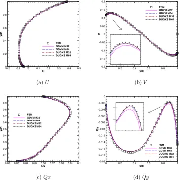
[image:9.595.120.489.56.424.2]

(10)

Fig.9. TheresultsofthecavityﬂowatKn=6.47×10−4₍_Re₌₄₀₀_):₍_a₎_U_-velocity_along_the_vertical_centerline,₍_b₎_V_-velocity_along_the_horizontal_centerline,₍_c₎_U_-velocity

contourand(d)V-velocitycontour.Intheﬁgures(c)and(d):background:theDUGKSresultswiththemeshof1282_;_the_black_solid_line:_the_DUGKS_results_with_the_mesh

642_;_the_white_{dash-double-dotted}_line:_the_GDVM_results_with_the_mesh_of₁₂₈2_;_the_rose_red_dash-dotted_line:_the_GDVM_results_with_the_mesh₆₄2_.

sameconclusion canbedrawnfortheﬂowsinthetransitionand freemolecularregimes.

TheresultsatKn=6.47×10−4 (Re=400)inthehydrodynamic regimearealsopresented,wherethebenchmarkNSsolutionsare available[46].Figs. 9(a) and(b)show thehorizontalandvertical velocityprofilesalongthecenterlinesofthecavity.Itisfoundthat withthecoarsemesh,theresultsofDUGKSaremuchbetterthan thoseofthe GDVM.Forexample,asshownin Fig.9(a), withthe meshof 322 , theGDVM underestimates the U-velocity boundary layeradjacentto thetopwall,whereastheDUGKScanaccurately capturethisvelocity boundary layer withsuch coarse resolution. ThisindicatesthattheGDVMismoredissipativethantheDUGKS. Inaddition,wealsoobservethattheDUGKSisnotsosensitiveto meshresolutions asthe GDVM.This isbecause that evenin this regime DUGKS still preserves the second-order spatial accuracy [34,35]. Similar observations can be obtainedfrom Figs. 9(c)and (d).Inthesetwofigures,we,respectively,plottheUandV veloc-itydistributions on different mesh resolutions; the well-resolved resultsofDUGKSwiththefinestmeshof1282 areregardedasthe referencesolutions.It is observedthat the resultsof GDVMwith a mesh of 642 clearly deviate from the reference solutions, par-ticularly around the cavitycorners and vortex centers, whilethe DUGKSwiththesamemeshcanadequatelyresolvetheflowfield.

ThisisconsistentwiththeanalysisinSection 2.4thattheDUGKS ismoreaccuratethantheGDVMinthecontinuumregime.

Fig. 10 gives the grid independent results of the U-velocity alongtheverticalcenterlineandtheV-velocityalongthe horizon-tal centerline, obtained from the GDVMand DUGKS simulations. The resultsarevalidatedby theDSMC data[45] forrareﬁedﬂow

(

Kn₌10_,1_,0_.1

)

andthe highresolutionNS data[46] for contin-uumﬂow

(

Re=400

)

.Itisclearlyfoundthat,withsuﬃcientgrids, theresultsof GDVMandDUGKS areinexcellent agreementwith thebenchmark solutions,andthenumberofgridpointsrequired bytheDUGKSisonlyhalfofthatfortheGDVM.

[image:10.595.103.489.52.437.2]

(11)

Fig.10. ThegridindependentresultsofU-velocityalongtheverticalcenterlineandV-velocityalongthehorizontalcenterline:(a)Kn=10,(b)Kn=1,(c)Kn=0.1and(d) Kn=6.47×10−4₍_Re₌₄₀₀_)._The_benchmark_results_from_the_DSMC_data_[45]_for_rarefied_flow_and_the_high_resolution_NS_data_given_by_Ghia_et_al._[46]_for_continuum_flow

arealsoincludedforcomparison.

Table2

Theratioofthegasmeanfreepathλandtheresolved gridsizexwhichgivesmeshindependentresults, de-notedbyδ=λ/x,atdifferentKnudsennumbers.

Kn 6.47×10−4 _0.0259 _0.1 ₁ ₁₀

δDUGKS 0.042 0.83 3.2 32 320

δGDVM 0.084 1.66 6.4 64 320

that therelations betweenresolved meshsize andgasmeanfree pathindifferentflowregimesareconsistentwiththeabove anal-ysis. Also, it is notedthat the DUGKSindeed requiresfewer grid pointstoresolvethegivenflowfield.

Distinct algorithm design of the GDVM andDUGKS may lead to differentconvergent processes.Fig.11depictsevolution ofthe relativeglobalerrordeﬁnedbyEq.(33)atdifferentKnudsen num-bers.InadditiontotheresultswiththesameCFLnumber,the re-sultsofGDVMwithalargeCFLnumberupto

η

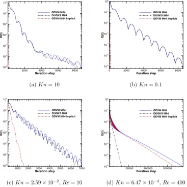
₌104_,_say_implicit GDVM, are alsoincluded.As wecan seefromFigs. 11(a) and(b), errorevolutionofbothmethodsinthetransitionandfree molec-ular regimes are almost identical to each other. However, when approaching to the slipand hydrodynamicregimes, as shownin Figs. 11(c)and (d), theconvergence rate ofDUGKS is apparently fasterthanthat oftheGDVM.Furthermore,wealsonote thatthe implicit GDVM converges about two orders of magnitude faster thantheGDVMandDUGKSinhighlyrareﬁedregime,whileinthe

continuumregion,asshowninFig.11(d),theconvergencerateof DUGKSturnstobetwotimesfasterthanthatofGDVMaswellas theimplicitGDVM.

Inadditiontoaccuracy,thecomputationalefficienciesofGDVM andDUGKSarealso measured.Firstly, we comparetheCPU time cost ofeach iteration. Fora faircomparison,the time stepis set tobeidenticalintheGDVMandDUGKS.ForthecaseofKn=0.1 with642 mesh points, the CPU time costs within one time step are0.1283s and0.2965 sforthe GDVMandDUGKS simulations, respectively, which indicates that the GDVM is about one time fasterthan theDUGKS for each iteration. According to our anal-ysisinSection 2.4,thisresultisnotsurprisingastheDUGKSwith afinite-volumeformulationcomputesmoreequilibriumstate func-tionsthanthefinite-differenceGDVM.

[image:11.595.120.489.55.423.2] [image:11.595.82.255.513.548.2]

(12)

Fig.11. ErrorevolutiondeﬁnedbyEq.(33)atdifferentKnudsennumbers:(a)Kn=10,(b)Kn=0.1,(c)Kn=2.59×10−2₍_Re₌₁₀₎_and₍_d₎_Kn₌₆_.₄₇_×₁₀−4₍_Re₌₄₀₀₎_.

NotethatfortheimplicitGDVM,theerrorisestimatedatonetimestep.

Table3

ThetotalCPUtimecosts(inminute)oftheGDVMandDUGKSwhenthe re-sultssatisfythestead-statecriteriongivenbyEq.(33)onthemeshof642_.

TheresultsoftheimplicitGDVMarealsoincluded.Notethattheconvergency criteriafortheimplicitGDVMismeasuredatonetimestep.

Kn 6.47×10−4 _0.0259 _0.1 ₁ ₁₀

tDUGKS 6.06 2.35 41.52 272.93 503.31

tGDVM 13.35 1.51 18.4 121.35 236.15

timplicit GDVM 11.92 0.20 0.35 1.2 4.01

tDUGKS/tGDVM 0.51 1.55 2.25 2.24 2.13

tDUGKS/timplicit GDVM 0.46 11.75 118.62 227.43 125.51

ofDUGKS.Moreover,itisinterestingtonotethatalthoughthe ef-ﬁciencyofimplicitGDVMisimprovedbytwoordersofmagnitude inhighlyrareﬁedregime,itisstillaboutonetimeslowerthanthe DUGKSinthehydrodynamicregime.

It should be noted that the above efficiency comparisons are based on the same mesh for the two methods. As shown, the GDVMrequires642 meshpointstoobtaintheresolvedresultsfor theflows fromearly slipto highlyrarefied regime, whilefor the DUGKS,itonlyneedsacoarsermeshof322 .Likewise,forthe con-tinuumflow,themeshrequirementsfortheGDVMandDUGKSare 1282 and642 ,respectively. Therefore,theDUGKScan achieve ac-curateresultswithcoarsermeshesincomparisonwiththeGDVM. Consequently, as shown in Table 4, to achieve the well-resolved results,the DUGKS is about one order of magnitude faster than

Table4

ThetotalCPUtimecosts(inminute)oftheimplicitGDVMandDUGKSwhenthe re-sultsarewellresolved.TheconvergencycriteriafortheimplicitGDVMismeasured atonetimestep.

Kn 6.47×10−4 _0.0259 _0.1 ₁ ₁₀

tDUGKS 6.06 0.31 6.17 35.7 58.38

timplicit GDVM 48.68 0.20 0.35 1.2 4.01

tDUGKS/timplicit GDVM 0.12 1.55 17.63 29.75 14.56

[image:12.595.111.479.58.427.2] [image:12.595.302.553.504.550.2]

theimplicitGDVMinthecontinuum region,andviceversainthe highlyrarefiedregime.Wemustemphasizethatalthoughthe uni-formmeshisusedintheabovesimulations, non-uniformmeshes canbe easilyimplemented inthefinite-differenceGDVMandthe finite-volume DUGKS [36]. In addition, the unstructured meshes have already been used for the DUGKS simulations [40]. It has been demonstrated that with nonuniform meshes, the efficiency ofDUGKScanbeimproveddramaticallytoallowlargesimulations [36,47].

[image:12.595.42.276.513.575.2]

(13)

4. Conclusions

The main objective of this work is to quantify the compu-tational performance of different DVMs, so that researchers may choosethemostappropriatemethodfortheirapplications.Our re-sultsshowthat boththeGDVMandDUGKScanaccurately repro-duce the results inall the ﬂow regimes,provided that themesh resolution issuﬃcient. Meanwhile, itis foundthat the DUGKSis less dissipative and consequently requires a much smaller num-berofgridpointsthantheGDVM,especiallyinthecontinuumand near-continuum regimes. For the GDVM, the convection term of thekineticmodelisapproximatedbytheupwindschemewiththe underlying assumption of molecular free streaming between two grid points, while in the DUGKSthe collision and transport pro-cesses are coupled physically by using the discrete characteristic solutionofthekineticequation.Therefore,evenwithathird-order discretization, the GDVM is not as accurate as the second-order DUGKS,particularlyinnearhydrodynamicregimes.

The efficiencyandconvergence rateofthe GDVMandDUGKS arealsocompared.Ourresultsshowthatwiththesamemeshfor each iteration, the CPU time cost of the DUGKS is about twice that ofthe GDVM, whichis not surprisingthat thefinite-volume DUGKS computes more equilibrium state distribution functions whencomparedtotheGDVMwithafinite-differenceformulation. Inaddition,whenusingthesametimestepandspatialmesh,the GDVM and DUGKSshow similar convergence rates for the flows ranging from thefree molecular to early slip, so that the GDVM is about twice as fast as the DUGKS; when using a large time step,theimplicitGDVMisfasterthantheexplicitDUGKSbyabout two ordersofmagnitude.However,astheflowapproachestothe hydrodynamicregimeinwhichmolecularcollisionsdominate,the DUGKSconvergesfaster,consequently, itturns outto betwice as fast as the implicit GDVM. It should be noted that in order to achieve results inreasonableaccuracy, theDUGKSrequires fewer meshpointsthanthe GDVM,therefore,theoverall computational efficiencyofDUGKScanbeimprovedbyoneorderofmagnitude.

Insummary,theDUGKSispreferableforflowproblems involv-ing differentflow regimes,whileifonly thesteady-statesolution ofhighlyrarefiedflowsisofinterest,theimplicitGDVM,whichcan boostthe GDVMconvergenceratebytwo ordersofmagnitude,is abetterchoice.

Acknowledgments

This work is ﬁnancially supported by the UK’s Engineering and Physical Sciences Research Council (EPSRC) under grants EP/M021475/1,EP/L00030X/1 andNationalNatural Science Foun-dationofChina(GrantNo.51125024).

References

[1] Bird GA. Molecular gas dynamics and the direct simulation ofgas Flows. Clarendon;1994.

[2] AlexanderFJ,GarciaAL,AlderBJ.Cellsizedependenceoftransportcoeﬃcients instochasticparticlealgorithms.PhysFluids1998;10(6):1540–2.

[3] ConnellST,ThompsonPA.Moleculardynamics–continuum hybrid computa-tions:atoolforstudyingcomplexﬂuidﬂows.PhysRevE1995;52(6):R5792.

[4] WeinanE,EngquistB,HuangZ.Heterogeneousmultiscalemethod:ageneral methodologyformultiscalemodeling.PhysRevB2003;67(9):092101.

[5] WerderT,WaltherJH,KoumoutsakosP.Hybridatomistic–continuummethod forthesimulationofdenseﬂuidﬂows.JComputPhys2005;205(1):373–90.

[6] BorgMK,LockerbyDA,ReeseJM.Ahybridmolecular–continuummethodfor unsteadycompressiblemultiscaleﬂows.JFluidMech2015;768:388–414.

[7] Radtke GA, Péraud J-PM, Hadjiconstantinou NG. On eﬃcient sim-ulations of multiscale kinetic transport. Philos Trans R SocLond A 2013;371(1982):20120182.

[8] MieussensL.Asurveyofdeterministicsolversforrarefiedflows.In: Proceed-ingsofthe29th InternationalSymposiumonRarefiedGasDynamics,1628; 2014.p.943.

[9] BroadwellJE.Studyofrareﬁedshearﬂowbythediscretevelocitymethod.J FluidMech1964;19(03):401–14.

[10]YangJ,HuangJ.RareﬁedﬂowcomputationsusingnonlinearmodelBoltzmann equations.JComputPhys1995;120(2):323–39.

[11]MieussensL.Discrete-velocitymodelsand numericalschemesforthe Boltz-mann-BGKequation inplane and axisymmetricgeometries. JComputPhys 2000;162(2):429–66.

[12] LiZ-H,ZhangH-X.Gas-kineticnumericalstudiesofthree-dimensional com-plexﬂowsonspacecraftre-entry.JComputPhys2009;228(4):1116–38.

[13]Meng J, Zhang Y,Hadjiconstantinou NG, Radtke GA, ShanX. Lattice ellip-soidalstatisticalBGKmodelforthermalnon-equilibriumﬂows.JFluidMech 2013;718:347–70.

[14]SoneY,OhwadaT,AokiK.TemperaturejumpandKnudsenlayerinarareﬁed gasoveraplanewall:numericalanalysisofthelinearizedBoltzmannequation forhard-spheremolecules.PhysFluidsA1989;1(2):363–70.

[15]AristovVV.DirectmethodsforsolvingtheBoltzmannequationandstudyof nonequilibriumﬂows,60.SpringerScience&BusinessMedia;2001.

[16]TcheremissineF.DirectnumericalsolutionoftheBoltzmannequation.Tech. Rep.DTICDocument;2005.

[17]MouhotC,PareschiL.FastalgorithmsforcomputingtheBoltzmanncollision operator.MathComput2006;75(256):1833–52.

[18]WuL,WhiteC,ScanlonTJ,ReeseJM,ZhangY.Deterministicnumerical solu-tionsoftheBoltzmannequationusingthefastspectralmethod.JComputPhys 2013;250:27–52.

[19]WuL,ReeseJM, ZhangY.Solving theBoltzmann equationdeterministically by the fast spectral method: application to gas microﬂows. J Fluid Mech 2014;746:53–84.

[20]Wu L, White C, Scanlon TJ, Reese JM, Zhang Y. A kinetic model of the Boltzmann equation for non-vibrating polyatomic gases. J Fluid Mech 2015;763:24–50.

[21]WuL,Zhang Y,Reese JM. Fast spectralsolutionofthegeneralized Enskog equationfordensegases.J.ComputPhys2015;303:66–79.

[22]BhatnagarPL, GrossEP,Krook M.Amodelfor collisionprocessesingases. I.Smallamplitudeprocessesinchargedandneutralone-componentsystems. PhysRev1954;94(3):511.

[23]HolwayJrLH.Newstatisticalmodelsforkinetictheory:methodsof construc-tion.PhysFluids1966;9(9):1658–73.

[24]ShakhovE.GeneralizationoftheKrookkineticrelaxationequation.FluidDyn 1968;3(5):95–6.

[25]XuK.Directmodelingforcomputationalfluiddynamics:constructionand ap-plicationofunifiedgas-kineticschemes.WorldScientific;2014.

[26]Chen S, Xu K. A comparative study of an asymptotic preserving scheme and uniﬁed gas-kinetic scheme in continuum ﬂow limit. J Comput Phys 2015;288:52–65.

[27]PieracciniS,PuppoG.Implicit–explicitschemesforBGKkineticequations.J SciComput2007;32(1):1–28.

[28]Dimarco G, Pareschi L. Asymptoticpreserving implicit-explicitRunge–Kutta methods for nonlinear kinetic equations. SIAM J Numer Anal 2013;51(2):1064–87.

[29]BennouneM,LemouM,MieussensL.Uniformlystablenumericalschemesfor the Boltzmannequation preservingthe compressibleNavier–Stokes asymp-totics.JComputPhys2008;227(8):3781–803.

[30]FilbetF,JinS.Aclassofasymptotic-preservingschemesforkineticequations andrelatedproblemswithstiff sources.JComputPhys2010;229(20):7625–48.

[31] XuK,HuangJ-C. Aunified gas-kineticscheme for continuum andrarefied flows.JComputPhys2010;229(20):7747–64.

[32]LiuS,YuP,XuK,ZhongC.Uniﬁedgas-kineticschemefordiatomicmolecular simulationsinallﬂowregimes.JComputPhys2014;259:96–113.

[33]ZhuY,ZhongC,XuK.Implicituniﬁedgas-kineticschemeforsteadystate so-lutionsinallﬂowregimes.JComputPhys2016;315:16–38.

[34]GuoZ,XuK,WangR.DiscreteuniﬁedgaskineticschemeforallKnudsen num-berﬂows:Low-speedisothermalcase.PhysRevE2013;88(3):033305.

[35]GuoZ,WangR,XuK.DiscreteuniﬁedgaskineticschemeforallKnudsen num-berﬂows.II.Thermalcompressiblecase.PhysRevE2015;91(3):033313.

[36]WangP,ZhuL,GuoZ,XuK.AcomparativestudyofLBEandDUGKSmethods fornearlyincompressibleﬂows.CommunComputPhys2015;17(03):657–81.

[37]Wang P, Tao S, Guo Z. A coupled discrete uniﬁed gas-kinetic scheme for Boussinesqﬂows.ComputFluids2015;120:70–81.

[38]GuoZ,XuK.Discreteuniﬁedgaskineticschemeformultiscaleheattransfer basedonthephononBoltzmanntransportequation.IntJHeatMass Transf 2016;102:944–58.

[39]WangP,WangL-P,GuoZ.ComparisonofthelatticeBoltzmannequationand discreteuniﬁedgas-kineticschememethodsfordirectnumericalsimulationof decayingturbulentﬂows.PhysRevE2016;94(4):043304.

[40]Zhu L, Guo Z, Xu K. Discrete uniﬁed gas kinetic scheme on unstructured meshes.ComputFluids2016;127:211–25.

[41]WangR.Uniﬁedgas-kineticschemefor thestudyofnon-equilibriumﬂows. TheHongKongUniversityofScienceandTechnology;2015.Ph.D.thesis.

[42]Zhu L,Wang P, GuoZ.Performance evaluation ofthe general characteris-ticsbasedoff-latticeBoltzmannschemeandDUGKSforlowspeedcontinuum ﬂows.JComputPhys2017;333:227–46.

[43]TitarevVA.Conservativenumericalmethodsformodelkineticequations. Com-putFluids2007;36(9):1446–59.

(14)

[45]JohnB,GuX-J,EmersonDR.Investigationofheatandmasstransferinalid– drivencavityundernonequilibriumﬂowconditions.NumerHeatTransf,Part B2010;58(5):287–303.

[46]Ghia U, Ghia KN, Shin C. High-Re solutions for incompressible ﬂow us-ing the Navier-Stokes equations and a multigrid method. J Comput Phys 1982;48(3):387–411.

[47]Bo Y, Wang P, Guo Z, Wang L-P. DUGKS simulations of three-dimen-sional Taylor–Greenvortexﬂow andturbulentchannelﬂow.Comput Fluids 2017;155:9–21.