Time-dependent variational approach for
Bose
–
Einstein condensates with nonlocal
interaction
Fernando Haas
1and Bengt Eliasson
21
Instituto de Física, Universidade Federal do Rio Grande do Sul, Av. Bento Gonçalves 9500, 91501-970 Porto Alegre, RS, Brasil
2
SUPA, Physics Department, University of Strathclyde, Glasgow G4 0NG, Scotland, United Kingdom E-mail:[email protected]
Received 25 February 2018, revised 24 June 2018 Accepted for publication 26 July 2018
Published 16 August 2018 Abstract
The nonlinear dynamics of self-bound Bose–Einstein matter waves under the action of an attractive nonlocal and a repulsive local interaction is analyzed by means of a time-dependent variational formalism. The mean-field model described by the Gross–Pitaevskii equation(GPE) is reduced to a single second-order conservative ordinary differential equation admitting a potential function. The stablefixed points and the linear oscillation frequencies of the breather modes are determined. The chosen nonlocal interactions are a Gaussian-shaped potential and a van der Waals-like potential. The variational solutions are compared with direct numerical simulations of the GPE, for each of these nonlocalities. The spatio-temporal frequency spectra of linear waves are also determined.
Keywords: Bose–Einstein condensate, matter wave, nonlocal interaction
(Somefigures may appear in colour only in the online journal)
1. Introduction
In many situations, nonlocal spatial interactions play a central role. In particular, the experimental observations of dipolar Bose–Einstein condensates (BECs) in systems composed of atoms with a large magnetic moment provided a breakthrough in ultra-cold gas physics [1–3]. The creation of self-bound quantum matter waves, or quantum balls [4], has become a concrete possibility to be realized in the near future. Proposals include the self-trapping of mesoscopic atomic clouds by a collective excitation of Rydberg atom pairs [5], additional interactions in dilute BECs of alkali atoms besides the dipolar interaction, creating 2D BEC solitons [6], the role of the orbital angular momentum on the arrest of collapse of vortex-free elliptical clouds of BECs described by Ermakov systems
[7, 8], and the manipulation of the atomic scattering length
through Feshbach resonance to produce stable solitons[9]. In a more general sense, nonlocality is present e.g.in nematic liquid crystals with long-range molecular forces[10], plasmas with a nonlocal response due to heating and ionization pro-cesses[11], the arrested collapse of ultra-cold magnetic gases due to quantumfluctuations[12], the crossover from a dilute BEC to a macrodroplet in a dipolar quantum fluid [13], the Rosensweig instability of quantum ferrofluids [14], ballistic transport of atoms[15], or the propagation of light beams in anisotropic nonlinear media [16]. Nonlocality is a decisive influence on the modulational instability of Kerr media [17], as well on the soliton stabilization and collapse arrest in nonlocal nonlinear systems[18].
In the present work, we analyze the nonlinear, time-dependent dynamics in a BEC with local and nonlocal interactions by means of a variational treatment, without external confinement. Previous studies in the literature on long-range interaction BECs include, for instance, descrip-tions restricted to the linear regime [6], specific interactions such as between dark solitons in dipolar BECs[19]by means of the direct simulation of the mean-field equation [20],
J. Phys. B: At. Mol. Opt. Phys.51(2018)175302(10pp) https://doi.org/10.1088/1361-6455/aad629
sian kernel, which is particularly well suited for detailed calculations. In addition, a nonlocal coupling reminiscent of the van der Waals potential[5,24,34] is also studied. The specific kernel does not qualitatively change our results, as seen in the comparison between the dynamics for Gaussian and van der Waals-like potentials(section4). Other possible nonlocal interactions include a Lorentzian shape [22] and singular 1/rncouplings, withn 1[25,35,36].
This work is organized as follows. In section 2, we introduce our basic mean-field model in terms of a nonlocal nonlinear Schrödinger equation and the associated variational formalism, with a Gaussian kernel. In section 3, a suitable time-dependent Ansatz is proposed for the wave function, which reduces the problem to a nonlinear second-order ordinary equation. Being conservative, the resulting dyna-mical system is associated with a potential function, which allows a sensible interpretation of the linear stability analysis results. Section4provides a numerical stability analysis of the variational solutions, by means of direct simulation of the original mean-field, nonlocal nonlinear Schrödinger equation. Section5 discuss the spectrum of linear excitations. Finally, section6contains our conclusions.
2. Variational approach
The Gross–Pitaevskii equation(GPE) with a nonlocal inter-action[37]term can be written as
¶y= -⎛ + y +
ò
- ¢ y ¢ ¢ y⎝
⎜ ⎞
⎠ ⎟ ∣ ∣ ( )∣ ( )∣
( )
i
M g W r r r d r
2 ,
1
t
2 2
2 2 3
whereÿis the reduced Planck constant,Mis the boson mass and g=4p2a M is the coupling constant in terms of the
boson–boson s-wave scattering length a. For simplicity we omit writing the explicit time-dependence of the wave func-tionψ(r,t)in equation(1)and in some equations below. We
first consider a Gaussian kernel specified by
- ¢ = ⎛- - ¢ ⎝
⎜ ⎞
⎠ ⎟
( ) ∣ ∣ ( )
W W
R
r r exp r r
2 , 2
0
2
2
where the constantsW0andRare, respectively, the strength and
range of the nonlocal interaction. Henceforth, we assumeg 0 andW0<0, so that the local(contact)and nonlocal couplings
are respectively repulsive and attractive. Although the sign and strength of g could be tuned by Fesbach’s resonance, we
will henceforth be applied:
t y y
⎛
⎝
⎜ ⎞
⎠
⎟ ( )
R t
t R
N
r r, , , 3
3 1 2
in terms of the characteristic time-scale t=MR2 , and
whereN= áy y∣ ñis the number of particles. The dimensionless GPE becomes
ò
y p g y
a y y
¶ = - +
- - - ¢ ¢ ¢
⎛ ⎝ ⎜
⎛ ⎝
⎜ ⎞⎠⎟ ⎞
⎠ ⎟ ( ) ∣ ∣
∣ ∣
∣ ( )∣ ( )
i
d
r r
r r
2 2
exp
2 , 4
t
2
3 2 2
2
2 3
using for simplicity the same symbols for the original and dimensionless quantities, together with the normalization
y y
á ∣ ñ =1, where a= -MNW R0 2 2>0 and g=
p
(2 )1 2Na R. Some numerical factors were calibrated
so that α=γrepresents a system where the local and non-local influences have the same order of magnitude, as found from inspection of equation (4) taking into account
ò
exp(-r2 2)d3r=(2p)3 2.The variational principle involves the action functional
*
ò
y y =
[ ]
S , dt d3r, where the Lagrangian density is
* * *
ò
y y y y y y p g y
a y y
= ¶ - ¶ -
-+ ⎛- - ¢ ¢ ¢
⎝
⎜ ⎞⎠⎟
( ) · ( ) ∣ ∣
∣ ∣ ∣ ∣
∣ ( )∣
( )
i
d
r r
r r
2 2
2 2
2 exp 2 .
5
t t
3 2 4
2 2
2 3
The functional derivative d dyS *=0 gives equation (4), whileδS/δψ=0 provides the complex conjugate of the GPE.
3. Radially symmetric states
A reasonable radially symmetric Ansatz is given by the Gaussian form
y
p s s b
= ⎛- +
⎝
⎜ ⎞⎠⎟
( ) ( )
r
i r
1
exp
2 , 6
3 2
2
2 2
which is properly normalized, whereσ=σ(t) (the width)and
β=β(t) are time-dependent variational functions to be determined. The function β is known as the chirp function
[39] and is necessary to obtain meaningful differential equations at the end of the time-dependent variational pro-cedure. In the stationary case (∂/∂t=0) one could chose
(see section 5), the chirp gives a radial contribution to the velocityfield, defined via the gradient of the complex phase (action)of the wave function.
Using equation (6) in (5) and integrating over space furnishes the LagrangianL=
ò
d3r, which is evaluated asb b
s s
g s
a s
= - + + - +
+
⎜ ⎟
⎛
⎝ ⎞⎠ ( )
( )
L 3
2 2
1
2 2 2 1 .
7
2 4
2
3 2 3 2
In passing, the integral of the nonlocal term was readily evaluated using the convolution theorem combined with the spatial Fourier transform(appendixA).
The Euler–Lagrange equation for β gives b=s˙ (2s), while∂L/∂σ=0 implies
s s
g s
a s
s s
= +
-+ =
-¶ 
( ) ( )
V
¨ 1
1 , 8
3 4 2 5 2
obtained after eliminatingβ. The pseudo-potential is
s s
g s
a s
= = +
-+ ( )
( ) ( )
V V 1
2 2 3 3 3 1 2 3 2. 9
The contributions can be clearly identified, namely: the
first(centrifugal)term in equation(9)is related to the kinetic energy of the condensate and would be neglected in the Thomas–Fermi approximation; the second term, proportional toγ, is due to the local, repulsive coupling; the third term, proportional toα, is due to the nonlocal, attractive coupling. We remark that in the case of an attractive contact interaction (γ<0)the total potential would be not bounded from below and no stable oscillations would be possible. This is due to the dominant contribution of the contact interaction ass0, as apparent in equations(8)and(9).
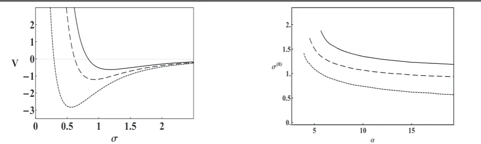
The total potential is illustrated in figure 1, where
α=20. Notice that increasing the interaction ratio
h g
a p
º =
( ) ∣ ∣ ( )
g R W
2 3 2 3 10
0
decreases the depth of the potential well. Therefore a strong nonlocal attractive potential leads to a more stably bound state, as expected.
In the general case, it is easy tofindη<1 as a necessary condition for obtaining stable minima ofV. Analytical results can be derived in specific cases. For very largeσ?1, equation(8) becomes s¨ =s-3+(g-a s) -4, which has a stable fixed
point σ=σ(0)=α−γ. On the other hand, for σ=1, equation (8) becomes s¨ +a s=s-3+g s-4, which is a Pinney equation[40]modified by an inverse quartic nonlinearity. In this situation,fixed points are determined byα σ5=γ+σ. If
γ?σ, then one would haves( )0 »(g a)1 5=h1 5, which is
consistently very small for a strong attractive nonlocal interac-tion. On the other hand, for negligible local interaction and
σ=1, one derivess( )0 »a-1 4.
[image:3.595.69.544.62.204.2]Figure2shows the location of the stablefixed pointσ(0) numerically obtained, as a function of the nonlocal interaction strength α, for a few choices of η. Notice that there is a minimum α allowing for periodic oscillations of the char-acteristic lengthσ. For instance, forη=0 one needsα 3.5. Moreover, a smaller η corresponds to a smaller condensate width, due to an enhanced attractive coupling. Figure3shows the corresponding angular frequency ω of the linear oscilla-tions, given byw2= ¶( 2V ¶s2)s s= ( )0. In particular, we note a higher frequency for largerα and smallerη.
[image:3.595.296.534.63.205.2] [image:3.595.330.518.271.406.2]Figure 1.Total potential from equation(9), forα=20 and different values of the interaction parameterη=γ/α. Upper, continuous curve:η=0.2; middle, dashed curve:η=0.1; lower, dotted curve:η=0.0.
[image:3.595.48.292.420.518.2]Figure 2.Minima of the potentialVin equation(9), as a function of αand different values of the interaction parameterη=γ/α. Upper, continuous curve:η=0.2; middle, dashed curve:η=0.1; lower, dotted curve:η=0.0.
fi
space by means of the convolution theorem, using the fast Fourier transform algorithm to numerically calculate the dis-crete Fourier transform and its inverse. A pseudo-spectral method is used to calculate the spatial derivatives. The pseudo-spectral method is very accurate as long as the solu-tion is well represented on the numerical grid. (Using equation(6), the width of the wave function in theFourier transformed spacecan be estimated to be approximately 1/σ, giving a width of the order 1–2; as seen e.g. in figure 2 at largeα. We are using a grid spacing ofΔx=5/16 giving the Nyqvist wavenumberπ/Δx≈10 which is much larger than the spectral width and therefore the solution is resolved well on the numerical grid.) A standard 4th-order Runge–Kutta scheme is used to advance the solution in time.
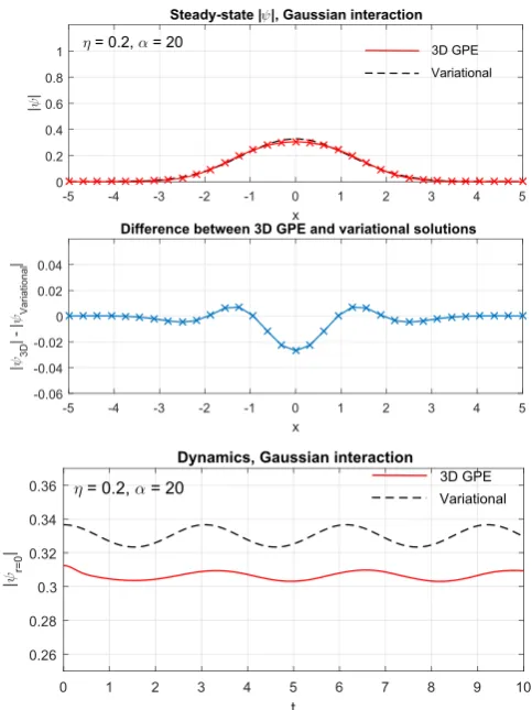
Figures4and5show the steady-state solutions of the GPE and variational systems, as well as the dynamics when the steady-state solutions are perturbed by 2%. The steady-steady-state of∣ ∣y is found by solving the GPE and by iteratively doing an averaging procedure ynew= (∣yt=t1∣2 +∣yt=t2∣2 ++ ∣yt=tN∣ )2 N, which enforces the normalizationáy y∣ ñ =1. The new solution
ψnewis then used as a starting point for a new iteration, until∣ ∣y converges to a time-stationary solution. The time difference tN−t1 is typically chosen to cover one oscillation period of
the system to efficiently damp out oscillations. Another averaging scheme is used for the variational solution, snew=
s= +s= ++ s=
( t t1 t t2 t tN) N, to find the steady-state
varia-tional solution. As seen in the top and middlefigures4–5, the comparisons between the 3D GPE solutions and the variational solutions are in general very good, with only minor deviations from the GaussianAnsatz. To compare the dynamics between the two approaches, the steady-state solutions were perturbed in a manner that the magnitude ofψis initially 2% larger than the equilibrium solution at the originx=y=z=0. For the varia-tional approach this is straightforward by choosing a suitable initial condition forσ. For the GPE the initial condition was set by acoordinate stretching procedure of the steady-state solution, again enforcing áy y∣ ñ =1 in the perturbed initial condition. Bottom panels offigures4–5show the time-evolution of∣ ∣y at the origin. Apart from a small difference in the steady-state solutions, the oscillation frequencies also agree to large degree, especially for the lower values ofη. Forη=0, one can also see oscillations with lower frequency in the 3D GPE solution, seen
first as a drift toward lower ∣ ∣y and then toward larger ∣ ∣y, indicating that the total(local plus nonlocal)nonlinear potential
of the deeply trapped condensate allows multiple oscillation modes.
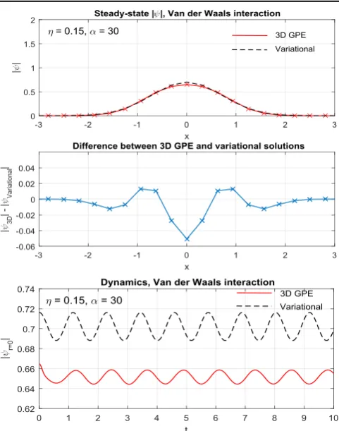
For comparison, we also carried out numerical simula-tions using a van der Waals-like interaction[5,24,34],
- ¢ =
+ - ¢ <
( ) ˜
∣ ∣
˜ ( )
W C
R C
r r
r r , 0 11
6
6 6 6
where C˜6 can be related to a strong van der Waals force
between Rydberg atoms, while R corresponds to the satur-ation of the effective interaction, due to the van der Waals shift(see[5]for details).
The 3D GPE in normalized units is
ò
y p g y a y y
¶ = - + - ¢ ¢
+ - ¢ ⎛
⎝
⎜ ∣ ∣ ∣ ( )∣ ⎞⎠⎟
∣ ∣ ( )
i r d r
r r
2 2
3 1 , 12
t
2 2
2
2 3
6
where a= -MNC˜6 (2R4)>0 and g=(6 p)Na R. Moreover,α=γcorresponds to the same order of magnitude of the contact and nonlocal couplings, since
ò
(1 +r6)-1 3d r=p
2 2 3.
Figure 4.Gaussian interaction withη=0 andα=20, showing the steady-state solution of∣ ∣y as a function ofxaty=z=0 obtained from the 3D GPE and variational solutions(top panel), the corresponding difference between the variational and 3D GPE solutions(middle panel), and the small-amplitude oscillations when the equilibrium is initially perturbed by 2%(bottom panel). The oscillations of the 3D GPE and variational solutions have a period of
=
The variational solution is based on the radially sym-metricAnsatzin equation(6). Proceeding in a similar manner as in section2 yields the Lagrangian
b b
s s
p g
s
s
= - ⎜⎛ + + ⎟ -
-⎝ ⎞⎠
( )
( )
L 3 U
2 2
1
2 2 6
3 2 ,
13
2 4
2
3
so thatb=s˙ (2s)and
s s
p g
s s
= + -
¶ ( )
U
¨ 1
2 3 , 14
3 4
in terms of the nonlocal interaction potential
ò
s = -a y ¢ y ¢
+ - ¢ ( ) ∣ ( )∣ ∣ ( )∣
∣ ∣ ( )
U r r d dr r
r r
3 1 . 15
2 2 3 3
6
An attractive contact interaction(γ<0)would prevent stable nonlinear oscillations, due to the dominant role of the σ−4 term in equation (14) when σ approaches zero. While U(σ) can be expressed in terms of hypergeometric functions[5], a numerically amenable form of the nonlocal interaction
potential is also (see appendix B)
ò
s = -a - s
-´ +
-¥
⎜ ⎟
⎛ ⎝
⎜ ⎞⎠⎟
⎡
⎣ ⎢ ⎢
⎛ ⎝
⎞ ⎠ ⎛ ⎝
⎜⎜ ⎛⎝⎜ ⎞
⎠
⎟ ⎛
⎝
⎜ ⎞
⎠ ⎟⎞
⎠ ⎟⎟⎤
⎦ ⎥ ⎥ ( )
( )
U k k
k k k
kdk
9 exp 2
1 exp
2 3 sin 3
2 cos 3
2 .
16
0
2 2
[image:5.595.307.547.63.389.2]The numerical results for the van der Waals-like nonlocal interaction are presented in figures 6 and 7. The GPE and variational steady-state solutions show excellent agreement forη=0 andα=30 infigure6, and also good comparison for η=0.15 as seen in figure 7. Also the dynamics show oscillation periods with high degree of agreements between the 3D GPE and variational solutions. Similar as for the Gaussian nonlocal interaction potential, one can also see a lower frequency oscillation in the 3D GPE solution for the caseη=0, indicating that the deeply trapped condensate has a more rich dynamics with more than one trapped oscilla-tory mode.
Figure 5.Gaussian interaction withη=0.2 andα=20, showing the steady-state solution of∣ ∣y as a function ofxaty=z=0 obtained from the 3D GPE and variational solutions(top panel), the corresponding difference between the variational and 3D GPE solutions(middle panel), and the small-amplitude oscillations when the equilibrium is initially perturbed by 2%(bottom panel). The oscillations of the 3D GPE and variational solutions have a period of
=
T3D 3.2444andTVariational=3.0731, respectively, corresponding to angular frequencies ofw3D=1.9366andwVariational=2.0446, with the variational frequency about 5.4% higher.
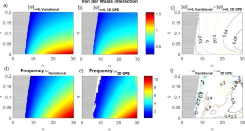
[image:5.595.49.291.65.388.2]A set of simulations, similar to the ones infigures4–7, were carried out for a range of different η andα to produce phase maps shown infigures8and9for the van der Waals interaction, respectively, showing the central amplitude ofψand the oscil-lation frequency for the variational and 3D GPE models. In general the agreement between the variational and 3D GPE solutions are good, with a typical deviation of about 5% or less.
5. Spectrum of elementary excitations
At this point and below it is more transparent to again employ physical variables. As a complementary study besides the search for localized nonlinear solutions, it is interesting to look for the linear wave spectrum around homogeneous equilibria of the GPE (1). This could be obtained using the Bogoliubov method[38]. Here we use an alternative method by employing the Madelung transformation[41]
y= n exp(iS ), (17)
ò
+
= - - - ¢ ¢ ¢ ¢
+
⎛ ⎝
⎜ ⎞
⎠ ⎟
⎛ ⎝
⎜ ⎞⎠⎟
( ) ( )
( )
M
n n g
M n M W n d
M
n n
r r r r
2
1
2 ,
19
2
3
2
2 2
where ¢ = ¶ ¶ ¢r and where in the last step an integration by parts was performed, assuming the nonlocal interaction to vanish at infinity.
Assuming
d d
= + = ( )
n n0 n, v v, 20
wheren0is a uniform equilibrium number density andδnand δvare small,first-order perturbations. Linearizing the system and letting the first-order perturbations be plane wave solu-tions proportional to exp[ ( ·i k r- Wt)], the result is the dispersion relation
W = n k ( + [ ])+ ( )
M g F W
k M
4 , 21
k
2 0 2 2 4
2
in agreement with [33], where F Wk[ ]=
ò
W( )r exp(-ik· )dr 3r denotes the Fourier transform of the nonlocal
interac-tion. In the absence ofWor for short wavelengths one regains the Bogoliubov spectrum.
5.1. Gaussian kernel
The hydrodynamic equations (18)–(19) and the linear dis-persion relation (21)are valid irrespective of the form of the nonlocal interaction. In the case of the model (2), the result from equation(21)is
p
W = ( +( ) (- ))+
( )
n k
M g W R k R
k M
2 exp 2
4 , 22
2 0 2 3 2
0 3 2 2
2 4
2
or, alternatively,
h
W = ⎛ - - +
⎝
⎜ ⎞
⎠ ⎟
( )
( )
c k k R k
M
1 exp 2
4 , 23
s
2 2 2 2 2 2 4
2
wherecs= g n0 M is the usual sound speed.
Expanding for long wavelengths, onefinds
h h
W = - + +
+ ⎛ ⎝
⎜ ⎞
⎠
⎟ ⎛
⎝
⎜ ⎞
⎠ ⎟
(( ) ) ( )
c k M c R k
M
k R
1 1 1 2
4
, 24
s
s
2 2 2 2
2 2
2
2 4
2
[image:6.595.50.291.62.368.2]6
Figure 8.Gaussian interaction, showing phase maps in the(α,η)parameter plane of the central amplitude ofψin(a)the variational model, (b)the 3D GPE model, and(c)contour map of the difference between the variational and 3D GPE solutions. Corresponding phase maps of the oscillation frequencies of the central amplitudes ofψin(d)the variational model,(e)the 3D GPE model, and(d)their difference. The shaded region at smallαindicate parameters for which no steady-state solutions are found.
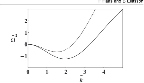
[image:7.595.56.547.424.687.2]which shows in a conclusive way an instability(Ω2<0)of long wavelengths ((k R)2=1), provided η<1. In conclu-sion, a strong attractive nonlocal interaction destabilizes homogeneous equilibria but allows the existence of stable nonlinear, self-trapped wave packets.
In terms of dimensionless variables W = W¯ t and =
¯
k k R, the wave spectrum is
p a
h
W =¯ ( ) n R k¯ ( - (-¯ ))+ ¯ ( )
N k
k
2
exp 2
4 , 25
2 3 2 0 3 2 2 4
which is shown in figure 10. It can be seen that a larger η reduces the unstable(W <¯2 0)region in wavenumber space.
5.2. Van der Waals-like kernel
The Fourier transform of the kernel shown in equation(11)is
p f
f =
º - +
-= - +
[ ] ˜ ( )
( ) ( )( ( ) ( )
( ) ( ))
( )
(( ) )
( )
F W C
R kR
kR kR
kR kR kR
kR kR
kR
k R
2
3 ,
exp
1 3 exp 2 sin 3 2
exp 2 cos 3 2
1
3 ,
26
k
2 6 3
2
4
yielding the long wavelength dispersion relation
h h
W = - + +
+ ⎛ ⎝
⎜ ⎞⎠⎟ ⎛
⎝
⎜ ⎞
⎠ ⎟
(( ) ) ( )
c k M c R k
M
k R
1 1 1 4
3 4
, 27
s
s
2 2 2
2 2 2
2
2 4
2
6
where now
h g
a p
= =
∣ ˜ ∣ ( )
R g C
3
2 . 28
3
2 6
Comparing equations(24)and(27), we conclude that the long wavelength dispersion relations for the two different kernels are basically the same, up a small discrepancy of order unity in the ∼k4term, provided the coupling parameter η is cor-rectly identified and the same characteristic lengthRis used.
In terms of dimensionless variables W = W¯ t and =
¯
k k R, the wave spectrum is
p a
h f
W =¯ n R k¯ ( - ( ¯))+ ¯ ( )
N k
k
2
3 4 , 29
2 2 0 3 2 4
which is shown in figure 11, with similar results as for the Gaussian kernel infigure10.
6. Conclusions
[image:8.595.320.551.55.188.2]In this work, the nonlinear dynamics of a completely self-bound (without external confinement) BEC with nonlocal coupling has been analyzed by means of a time-dependent variational formalism. For definiteness, the nonlocal and contact interactions were assumed to be respectively attractive and repulsive, but the proposed method can be easily adapted to alternative situations. It is found that the problem is always reducible to a nonlinear oscillator with a linearly stable equilibrium, whose location and breather frequency can be determined in great detail, specially for a nonlocal Gaussian-shaped kernel, which is more amenable to analytical calcu-lations. A van der Waals-like interaction was also considered, which can be related to an attractive effective force in mesoscopic atom clouds due to off-resonant dressing to RydbergnDstates[5]. We have made a comparison between the approximate, variational solutions and the output from the direct simulation of the nonlocal GPE. As a complement to the nonlinear analysis, the linear spectrum of spatio-temporal waves was also addressed and shown to be determined by the Fourier transform of the nonlocal potential. In this context, the Gaussian and van der Waals-like couplings were shown to yield essentially similar dispersion relations. The present results provide insight for the engineering of self-trapped matter waves. Topics to be addressed in future works include the analysis of the existence and stability of BECs with non-radial, rotational states, twisted phonons carrying a finite angular momentum[42], vortex-phonon interactions[43]and twisted nonlinear waves [44], in BECs with long-range interactions.
Figure 10.Dimensionless dispersion relation for the Gaussian kernel, from equation(25), with(2p)3 2an R N=1
0 3 andη=0.1
(continuous line),η=0.3(dashed line).
Figure 11.Dimensionless dispersion relation for the van der Waals interaction, from equation(29), with2p a2 n R (3N)=1
0 3 andη=0.1
[image:8.595.50.272.63.190.2]Acknowledgments
FHacknowledges the support by Conselho Nacional de Desenvolvimento Científico e Tecnológico (CNPq). BE acknowledges support from the Engineering and Physical Sci-ences Research Council (EPSRC), grant nr EP/M009386/1. Data supporting thefigures can be found athttp://doi.org/10. 15129/df750efc-d1f5-48cf-8ba6-6f9cf498011e. Bengt Eliasson ([email protected]) can be contacted directly with queries about the data.
Appendix A. Evaluation of Lagrangian function(7) The Lagrangian shown in equation(7)can be obtained from equations (5) and (6) in a straightforward way with the exception of the term associated with the nonlocal interaction. This one can be obtained by brute force integration using e.g. Cartesian coordinates and evaluating the several integrals over Gaussian functions or by a more gentle approach considering the convolution theorem, as follows. Let the functions
y
= =
-( ) ∣ ( )∣ ( ) ( ) ( )
n r r 2, K r exp r2 2 A1
and their convolution
ò
* = - ¢ ¢ ¢ =
-( ) ( ) ( ) [ ( ) ( )]
( )
K n K r r n r d r F F K F n ,
A2
r 3 1
where the last equality is due to the convolution theorem, in terms of
ò
= =
-( ) ˆ ( ) ( ) · ( )
F f f k f r e ik rd3r, A3
which is the Fourier transform of a generic functionf(r)with
ò
p= =
-( ˆ ) ( )
( ) ˆ ( ) ( ) ·
F f f r 1 f k e d k
2 A4
ik r 1
3
3
denoting its inverse. Considering the Gaussian trial wave function in equation(6), we obtain
s s * = + - + ⎡ ⎣ ⎢ ⎤⎦⎥ ( ) ( ) ( ) ( )
K n 1 r
1 2 exp 2 1 2 A5
r 2 3 2
2
2
and then
ò
(K * n n) ( )r d r=(1 +s )- , (A6)r 3 2 3 2
which yields the Lagrangian in equation(7).
Appendix B. Evaluation of pseudo-potential(16) The pseudo-potential shown in equation(16)can be obtained from equation(15)by applying the convolution theorem and Parseval’s formula, as follows. Let the functions
y = = + ( ) ∣ ( )∣ ( ) ( ) n K r
r r , r 1
1 . B1
2
6
Then equation(15)can be written
ò
s = -a *
( ) ( )( ) ( )
U n r K n d r
3 r B2
3
in terms of the convolution product
ò
* = - ¢ ¢ ¢ =
-( ) ( ) ( ) [ ( ) ( )]
( )
K n K r r n r d r F F K F n ,
B3
r 3 1
where the last equality is due to the convolution theorem, in terms of the Fourier transform pair
ò
= =
-( ) ˆ ( ) ( ) · ( )
F f f k f r e ik rd3r, B4
ò
p= =
- ( ˆ ) ( )
( ) ˆ ( ) ( ) ·
F f f r 1 f k e d k
2 . B5
ik r 1
3
3
It should be noted that bothn(r)and K(r)and their Fourier transforms nˆ ( )k and Kˆ ( )k are spherically symmetric, real-valued functions that only depend on the modulus of their arguments. Planckerel’s(Parseval’s)formula
ò
ò
ò
p p p = = = ¥( ) ˆ ( ) ˆ( )
( ) ˆ ( ) ˆ( ) ( )
fg d f g d
f k g k k dk
r 1 k k k
2 4
2 k , B6
3
3
3
3 0
2
where spherical coordinates were introduced in the last step, is then applied to equation (B2)to give
ò
s pa p = -= ¥ ( )( ) ˆ ( ) ˆ ( ) ( )
U 4 n k K k k dk
3 2 3 k 0 , B7
2 2
where
s
=
-ˆ ( ) ( ) ( )
n k exp k2 2 4 B8
and p = - + -⎜ ⎟ ⎡ ⎣ ⎢ ⎢ ⎛ ⎝ ⎞ ⎠ ⎛ ⎝ ⎜⎜ ⎛⎝⎜ ⎞ ⎠ ⎟ ⎛ ⎝ ⎜ ⎞ ⎠ ⎟⎞ ⎠ ⎟⎟⎤ ⎦ ⎥ ⎥ ˆ ( ) ( )
( ) K k k k k k k 2
3 exp 1 exp 2 3 sin 3 2
cos 3
2 . B9
2
Using equations (B8) and (B9) in (B7) yields the pseudo-potential in equation (16).
ORCID iDs
Fernando Haas https://orcid.org/0000-0001-8480-6877 Bengt Eliasson https://orcid.org/0000-0001-6039-1574
References
[1] Lahaye T, Menotti C, Santos L, Lewenstein M and Pfau T 2009Rep. Prog. Phys.72126401
[2] Baranov M A, Dalmonte M, Pupillo G and Zoller P 2012 Chem. Rev.1125012
[12] Ferrier-Barbut I, Kadau H, Schmitt M, Wenzel M and Pfau T 2016Phys. Rev. Lett.116215301
[13] Chomaz L, Baier S, Petter D, Mark M J, Wächtler F, Santos L and Ferlaino F 2016Phys. Rev.X6041039
[14] Kadau H, Schmitt M, Wenzel M, Wink C, Maier T, Ferrier-Barbut I and Pfau T 2016Nature530194
[15] Skupin S, Saffman M and Krolikowski W 2007Phys. Rev. Lett.98263902
[16] Mamaev A V, Saffman M, Anderson D Z and Zozulya A A 1996Phys. Rev.A54870
[17] Krolikowski W, Bang O, Rasmussen J J and Wyller J 2001 Phys. Rev.E64016612
[18] Bang O, Krolikowski W, Wyller J and Rasmussen J J 2002 Phys. Rev.E66046619
[19] Bland T, Edmonds M J, Proukakis N P, Martin A M, O’Dell D H J and Parker N G 2015Phys. Rev.A92063601
[20] Edmonds M J, Bland T, O’Dell D H J and Parker N G 2016 Phys. Rev.A93063617
[21] Pérez-Garcia V M, Konotop V V and Garcia-Ripoll J J 2000 Phys. Rev.E624300
[22] Parola A, Salasnich L and Reatto L 1998Phys. Rev.A57 R3180
[23] Köberle P, Zajec D, Wunner G and Malomed B A 2012Phys. Rev.A85023630
New J. Phys.15083055
[31] Buccoliero D, Desyatnikov A S, Krolikowski W and Kivshar Y S 2007Phys. Rev. Lett.98053901
[32] Buccoliero D and Desyatnikov A S 2009Opt. Express179608
[33] Picozzi A and Rica S 2012Opt. Commun.2855440
[34] Biswas A, Das T K, Salasnich L and Chakrabarti B 2010Phys. Rev.A82043607
[35] Maucher F, Skupin S, Shen M and Krolikowski W 2010Phys. Rev.A81063617
[36] Maucher F, Skupin S and Krolikowski W 2011Nonlinearity
241987
[37] Landau L and Lifschitz L 1996Statistical Physics(Oxford: Butterworth-Heinemann)
[38] Pethick C J and Smith H 2002Bose–Einstein Condensation in Dilute Gases(Cambridge: Cambridge University Press)
[39] Anderson D 1983Phys. Rev.A273135
[40] Pinney E 1950Proc. Am. Math. Soc.1681
[41] Madelung E 1926Naturwissenschaften141004
[42] Mendonça J T and Gammal A 2014J. Phys. B: At. Mol. Opt. Phys.47065301
[43] Mendonça J T, Haas F and Gammal A 2016J. Phys. B: At. Mol. Opt. Phys.49145302