City, University of London Institutional Repository
Citation:
Kerr, O. & Gumm, Z. (2017). Thermal instability in a time-dependent base state
due to sudden heating. Journal of Fluid Mechanics, 825, pp. 1002-1034. doi:
10.1017/jfm.2017.408
This is the accepted version of the paper.
This version of the publication may differ from the final published
version.
Permanent repository link:
http://openaccess.city.ac.uk/17471/
Link to published version:
http://dx.doi.org/10.1017/jfm.2017.408
Copyright and reuse: City Research Online aims to make research
outputs of City, University of London available to a wider audience.
Copyright and Moral Rights remain with the author(s) and/or copyright
holders. URLs from City Research Online may be freely distributed and
linked to.
City Research Online:
http://openaccess.city.ac.uk/
[email protected]
Thermal instability in a time-dependent base
state due to sudden heating
By O L I V E R S. K E R R
A N DZ O ¨
E G U M M
Department of Mathematics, City, University of London,Northampton Square, London EC1V 0HB, U.K.
(Received 31 May 2017)
When a large body of fluid is heated from below at a horizontal surface the heat diffuses into the fluid, giving rise to a gravitationally unstable layer adjacent to the boundary. A consideration of the instantaneous Rayleigh number using the thickness of this buoyant layer as a length scale would lead one to expect that the heated fluid is initially stable, and only becomes unstable after a finite time. This transition would also apply to other situations, such as heating a large body of fluid from the side, where a buoyant upward flow develops near the boundary. In such cases when the evolving thermal boundary layer first becomes unstable the time-scale for the growth of the instabilities may be comparable to the time-scale of the evolution of the background temperature profile, and so analytical approximations such as the quasi-static approximation, where the time-evolution of the background state is ignored, are not strictly appropriate.
We develop a numerical scheme where we find the optimal growth of linear pertur-bations to the background flow over a given time interval. Part of this problem is to determine an appropriate measure of the amplitude to the disturbances, as inappropri-ate choices can lead to apparent growth of disturbances over finite time intervals even when the fluid is stable. By considering the Rayleigh–B´enard problem, we show these problems can be avoided by choosing a measure of the amplitude that uses both the velocity and temperature perturbations, and which minimizes the maximum growth.
We apply our analysis to the problems of heating a semi-infinite body of fluid from horizontal and vertical boundaries. We will show that for heating from a vertical boundary there are large and small Prandtl number modes. For some Prandtl numbers both modes may play a role in the growth of instabilities. In some cases there is transition during the evolution of the most unstable instabilities in fluids such as water, where initially the instabilities are large Prandtl number modes and then morph into small Prandtl number modes part of the way through their evolution.
1. Introduction
When a layer of fluid between two horizontal boundaries is heated from below con-vection instabilities can arise. This is the well known Rayleigh–B´enard problem. When the temperature difference across the fluid passes a critical level instabilities can develop. This critical value is expressed in terms of the Raleigh number
Ra= gα∆T H 3
νκ , (1.1)
viscosity andκthe thermal diffusivity. The well-known critical Rayleigh number for this problem being Ra = 27π4/4 for stress-free boundaries and Ra = 1707.8 for no-slip boundaries (see, for example, Drazin & Reid 1981).
When a semi-infinite body of fluid is heated from below by a sudden increase in tem-perature at its horizontal boundary, the heat diffuses into the fluid, penetrating a distance of order (κt)1/2from the boundary wheretis the time since the onset of heating. A sim-plistic argument would suggest that as this buoyant layer has a depthH =O (κt)1/2
the effective Rayleigh number grows as t3/2. This would mean that the thermal layer would start off being stable, and become unstable at a later time.
The transition from stability to instability some time after the initial application of a destabilizing effect has been observed experimentally in other situations. For example, in the experiments of Chen, Briggs & Wirtz (1971), water with a vertical salinity gradient was heated from a vertical boundary. In one example, shown in their figure 8(b), insta-bilities are observed to start forming in the middle of the wall around 8 minutes after the wall temperature was raised. In the related experiments of Narusawa & Suzukawa (1981), where a constant heat flux was applied at a vertical wall bounding a salinity gradient, the authors observed instabilities first appearing in some cases an hour or more after the onset of heating. In both these cases the background state is intrinsically unsteady.
The linear stability analysis for the Rayleigh–B´enard problem is made simpler because there exists a background state that is steady — the conduction solution. In these cases it is common to be able to perform a normal mode analysis, where the form of the instability can be separated into a time-dependent part and a spatial part, with the growth of the disturbances being exponential in time. For a steady background state, an exponentially growing linear instability will eventually reach a finite amplitude where it can be observed and nonlinearity becomes important. In this case the concept of marginal stability — the condition separating the situation where no modes grow exponentially from cases where at least one mode grows — is important. There are many examples of investigations of the stability of steady flows and background states in many branches of fluid mechanics (again see, for example, Drazin & Reid 1981).
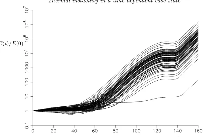
numeri-E(t)/E(0)
[image:4.595.100.434.110.336.2]t
Figure 1.The growth of the size of 100 sets of instabilities when a semi-infinite body of fluid is heated from a vertical wall subject to random perturbations. Each realisation differs only in the seed for the random number generator for the noise. Further details provided in§5.
cally is to subject a simulation of the background flow to random noise and to look at the evolution of instabilities. This was used by, for example, Kim & Kim (1986) in an investigation of the heating of a layer of fluid from below. They applied a constant heat flux at the heated boundary, while here we will apply a fixed temperature rise. In figure 1 are shown the results of 100 such runs for one of the problems under consideration here: the heating of a semi-infinite body of fluid from a vertical sidewall. The details of these calculations will be left to the relevant section of this paper. These calculations show the evolution of an energy-like measure of the amplitude of the disturbances renormalised so that they all start at 1 whent = 0, the time of the onset of wall heating. The only differences between all these runs is the value of the seed number used in the random number generator. Even if we ignore the outlying curve at the bottom, These exhibit a significant spread of amplitudes at t = 160. If one were to look for the time when instabilities start to grow, or the time they take to reach a given threshold ofE(t)/E(0), there would also be a high level of uncertainty. The approach that we will take in this paper aims to provide well-defined answers to these points.
In this paper we will primarily be concerned with two convection problems. Firstly, the case of heating a large body of fluid from below at a horizontal boundary. Secondly, we will look at the related problem where the heating is from a vertical wall. Before we do this we will outline the method that we use. This involves following the evolution of all possible linear instabilities from an initial time, t0, (which may or may not be the time of the onset of heating) to some later time,t1. For some measure of the amplitude of the disturbances, we will then find the optimum initial conditions that give rise to the maximum growth over this time interval.
of initial perturbations to the velocity, and no initial perturbations to the temperature. We will see that this approach will tend to underestimate the growth.
The use of non-modal stability theory to look at the transient growth of instabilities has been looked at by numerous authors (see Schmid 2007, for a review). In particular relevance here is the analysis of time-evolving problems by deriving the set of adjoint differential equations for the problem under consideration, and then developing an itera-tive scheme where the initial value problem is solved forwards in time using the original equations and using the final solution thus found to give the initial conditions for the adjoint problem. This was then solved backwards in time to the initial point, which in turn provides the initial conditions for solving the original differential equations for the next iteration. This approach has been reviewed in Luchini & Bottaro (2014). This approach was used to look time dependent Rayleigh–B´enard–Marangoni convection by Doumenc, Boeck, Guerrier & Rossi (2010). It will be seen that this method is funda-mentally equivalent to the approach taken here, however the formulation of the problem and the numerical approach are quite different. No adjoint differential equations will be derived or explicitly solved here.
In§2 we will set out the basic convection problems we will consider, and the numerical approach taken to find the optimum disturbances. We will then apply this approach in
§3 to the classic Rayleigh–B´enard problem to verify the approach. It will be seen how the growth predicted is dependent on the choice of the measure of the amplitude, and that an inappropriate choice of this measure can lead to over-predictions of growth, even predicting growth in stable systems. Considering a problem with a time-independent background state enables some of the features, and potential drawbacks, of measures of the amplitude to be examined without the confounding effects of an evolving background state. When the measure is chosen appropriately the analysis will reveal the exponential growth found by more conventional analysis, even for growth over quite restricted time intervals.
In§4 we will apply the methods developed to the investigation of the problem of heating a semi-infinite body of fluid from a horizontal lower boundary, and in §5 the problem of heating a semi-infinite body of fluid from a vertical boundary. Again, a warm layer develops near the boundary, but in this case the buoyant region generates an up-flow near the wall. We will mainly focus on results for the case of Prandtl numberσ=ν/κ= 7, which is appropriate for water, but also has a relatively complex behaviour for the sidewall problem where the instabilities observed straddle two different regimes. We will also look at the trends for more general Prandtl numbers.
2. Problem formulation and solution method
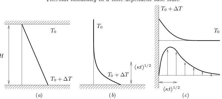
We will look at three basic problems. Firstly we consider the heating of a horizontal layer of fluid from below. This is the classic Rayleigh–B´enard problem as shown schemat-ically in figure 2(a). The second case is where we look at the heating of a semi-infinite body of fluid from a single horizontal boundary below the fluid. In this situation there is a growing destabilizing temperature gradient of height of order (κt)1/2 wheret is the time since the onset of heating andκthe thermal diffusivity. This is shown schematically in figure 2(b). The last case is where a semi-infinite body of fluid is heated from a vertical side wall, shown schematically in figure 2(c). Again there is a growing buoyant layer of fluid next to the boundary of width (κt)1/2, which, in this case, causes the fluid near the wall to rise. We will look at the growth of linear perturbations to these background states.
H 000000000000000 000000000000000 111111111111111 111111111111111 000000000000000 111111111111111 000000000000000 111111111111111 000000 000000 000000 000000 000000 000000 000000 000000 000000 000000 000000 000000 000000 000000 000000 111111 111111 111111 111111 111111 111111 111111 111111 111111 111111 111111 111111 111111 111111 111111 0 0 0 0 0 0 0 0 0 0 0 0 0 0 1 1 1 1 1 1 1 1 1 1 1 1 1 1 T0
T0+ ∆T
000000000000000 000000000000000 111111111111111 111111111111111
T0
T0+ ∆T
(κt)1/2
(κt)1/2
0000000000000000000 0000000000000000000 1111111111111111111 1111111111111111111 0 0 0
0 1 1 1
1
T0
T0+ ∆T
[image:6.595.104.466.112.274.2](a) (b) (c)
Figure 2.Schematic diagrams showing the temperature profiles for (a) Rayleigh–B´enard con-vection between two parallel horizontal plates, (b) heating from a single lower boundary, and (c) the temperature profile (upper line) and velocity profile (lower line) for heating from a single vertical wall.
T, for all the cases are
∂u
∂t +U(x, t)· ∇u+u· ∇U(x, t) =−
1
ρ0∇
p+gαTˆz+ν∇2u, (2.1a)
∇ ·u= 0, (2.1b)
∂T
∂t +U(x, t)· ∇T +u· ∇T(x, t) =κ∇
2T, (2.1c)
here U(x, t) and T(x, t) are the background velocity and temperature profiles, g the acceleration due to gravity, αthe coefficient of thermal expansion,ν the kinematic vis-cosity, ρ0 the density at temperature T0, and ˆz a unit vector pointing upwards. Here we have made the Boussinesq approximation and assumed a linear equation of state. For the horizontal layer we look at instabilities to the steady-state case where the lower boundary atz= 0 is held at a temperatureT0+ ∆T, while the upper boundary atz=H is kept atT0. For the two cases of single boundaries we consider the case of a stationary fluid which initially has a uniform temperature T0, and, at some initial timet= 0, the boundary temperature is increased toT0+ ∆T and held at this level.
The boundary conditions for the disturbances that we consider are that the velocity and temperature perturbations are zero at the solid boundaries, and tend to zero away far from the walls for the semi-infinite cases.
In this study we will restrict ourselves to looking at two-dimensional motions, and so we can use the vorticity–streamfunction formulation. We take the curl of the momentum equation (2.1a) and consider they-component of the vorticity,ω. We will nondimension-alize the equations using the rescalings
x′
=x/D, t′
=κt/D2, ω′
=D2ω/κ, T′
=T /∆T. (2.2)
where D is an appropriate length-scale. For the case of two parallel boundaries the distance between the walls,H, is an obvious and conventional choice of a length-scale for nondimensionalizing the equations. For the case D = H we derive the nondimensional equations for the vorticity and the streamfunction,ψ′
:
1
σ
∂ω′ ∂t′ −
∂ψ′ ∂z′
∂2W′ ∂x′2 +W
′∂ω ′
∂z′
=−Ra∂T ′
∂x′ +∇ ′2ω′
∇′2ψ′
=−ω′
, (2.3b)
where the primes indicate nondimensional variables. The perturbation velocity compo-nents are given by
u′
=−∂ψ
′
∂z′, w ′
= ∂ψ
′
∂x′. (2.4)
The vertical component of the background velocity,U′, is denoted by W′. This is only non-zero for the vertical sidewall problem.
Here the Rayleigh number,Ra, is the nondimensional measure of the heating, defined by (1.1). For the case of a semi-infinite fluid the length-scale H is not available. For an evolving system that has the heating turned on at some initial time the distance the heat diffuses into the fluid is of order (κt)1/2. This length-scale steadily increases. If we were to imagine this being substituted into the Rayleigh number then we would see that the Rayleigh number would start from zero, and increase without bound. Thus we may expect that the fluid would start stable and become unstable at some point when the Rayleigh number passes some critical value. If we choose the Rayleigh number being 1 as giving us an indication of when we may expect instabilities to form, then this gives us the corresponding length-scale
L=
νκ gα∆T
1/3
. (2.5)
This is the scale used by Foster (1965, 1968). If we useD=Lthen the nondimensional equations would be the same as (2.3), but without the Rayleigh number.
For the Rayleigh–B´enard problem the difference in using the length scale (2.5) as opposed toHwould be that the upper boundary conditions would be imposed atz=H/L
instead of the more conventional z = 1. The stability problem would then consist of finding the critical value of H/L above which the fluid would be unstable instead of finding the critical value ofRa. For the classical Rayleigh–B´enard problem these critical values are related byH/L=Ra1/3.
The perturbation temperature equation for both cases with horizontal boundaries is given by
∂T′ ∂t′ +
∂ψ′ ∂x′
∂T′ ∂z′ =∇
′2T′
, (2.6)
and for vertical boundaries by
∂T′ ∂t′ −
∂ψ′ ∂z′
∂T′ ∂x′ +W
′∂T′
∂z′ =∇ ′2T′
. (2.7)
Henceforth we will drop the primes.
far wall the vorticity is located near the heated wall for the semi-infinite cases, dropping from the peak value by, typically, five orders of magnitude towards the far wall of the computational domain. Hence, in the far field, the streamfunction satisfies∇2ψ≈0. By using the fact that the vorticity is minimal at this far wall we set the numerical condition that it is zero, and allowing non-zero ψ that decays exponentially as e−αz or e−αx as
appropriate by setting the derivative ofψto−αψ. In this way we can further reduce the effect on the solution of using a finite domain.
In general we allow for initial conditions for the perturbations to be applied at some time, t0, after the start of heating, although for many of our calculations we will set
t0 = 0. We then monitor the growth in the magnitude of the disturbances by using a suitable measure, which can be thought of as being like a generalised “energy” of the disturbances. For a fluid heated from a horizontal boundary in a semi-infinite fluid we will use
E(t) = 1 2P
Z ∞
0
Z P
0 |
u|2+λT2dx dz, (2.8)
whereP = 2π/αis the horizontal periodicity of the disturbances. If we take the vorticity to be the real part ofω(z, t)eiαx, with similar definitions forψandT, then we can write
(2.8) as
E(t) = 1 4
Z ∞
0
ψrωr+ψiωi+λ Tr2+Ti2
dz=EK(t) +λET(t), (2.9)
where ψr and ψi are the real and imaginary parts of ψ(z, t), and similarly for ω and T. The square root of this integral is a weighted norm of the disturbances where the positive parameterλis as yet unspecified. For instabilities between two horizontal plates the upper limit in the integral is replaced by the location of the upper boundary. For a semi-infinite fluid heated from a vertical wall the roles of xandz are swapped in (2.8) and (2.9). Other measures could be used, for example the enstrophy could replace the kinetic energy,EK(t). These alternatives are not considered here.
Our objective is to find the optimal perturbation at t0 to give the greatest growth in this “energy” at some later timet1. In the studies of Foster (1965, 1968) the focus was in the growth of the kinetic energy of disturbances that were initiated at t0 = 0 with no temperature perturbation. This is equivalent to setting λ = 0 and restricting perturbations in the initial conditions to the vorticity only.
We express the numerical solution at the interior points as a vector
Ψ(t) = (Tr1, Tr2, . . . , Tr N, Ti1, Ti2, . . . , TiN, ωr1, ωr2, . . . , ωr N, ωi1, ωi2, . . . , ωiN)T,
(2.10) where N is the number of interior points. For heating from horizontal boundaries the lateral symmetry allows us to simplify the problem by setting, say, the real part ofT and the imaginary parts ofωandψto zero. We can then express the numerical approximation to the “energy” as
E(t) =Ψ(t)TA(λ)Ψ(t) (2.11)
for an invertable symmetric matrix A(λ), where T indicates the transpose. Note: the
symmetry of this matrix is due to the numerical scheme used here. Other numerical schemes, for example ones using a non-uniform grid, may lead to an asymmetricA. This
has a small effect on the analysis which is mentioned below.
solution att=t1 is linearly dependent on the vector representation att=t0, and so we have
Ψ(t1) =MΨ(t0) (2.12)
for some transfer matrixM. We findM by performing repeated calculations of the
nu-merical scheme with the initial conditions, Ψ(t0), chosen so that one component is set to 1, with all other components set to 0. Each vector, Ψ(t1), found by calculating the evolution one of these initial conditions then gives the column of the transfer matrix,
M, corresponding to the non-zero initial component. Because of the translational
sym-metry of the problem, we only need to perform these calculations to find the columns of M corresponding to, say, the components of Tr and ωr being set to 1. The columns
corresponding to the components Ti and ωi being perturbed can then be inferred
di-rectly from these. The numerical calculation of this transfer matrix lends itself to simple parallelisation.
We can now express our optimisation problem as finding the vectorΨwhich maximizes (MΨ)TA(MΨ) with ΨTAΨ = 1. (2.13)
Using a Lagrange multiplier,µ, this maximization problem requires finding the solution to
MTAMΨ=MTAMA−1(AΨ) =µAΨ, (2.14) an eigenvalue problem with eigenvectorAΨ. If the numerical method used has an
asym-metric A then the resulting eigenvalue problem replaces A with its symmetric part:
1
2 A+AT
.
If we pre-multiply (2.14) byΨTwe find
ΨTMTAMΨ = (MΨ)TA(MΨ) =µΨTAΨ =µ. (2.15)
From this it is clear the maximum growth in “energy”,E(t1), is also the largest eigenvalue,
µ. As all the eigenvalues are positive, we can find an eigenvectorΦ=AΨ with the largest
eigenvalue by the iteration scheme
Φn+1=
MTAMA−1Φ
n |MTAMA−1Φ
n|
. (2.16)
The initial values of the problem,Ψ, can then be determined by multiplyingΦ byA−1 and rescaling to ensure thatE(t0) = 1. We will assume henceforth thatE(t0) = 1 in all cases, and soE(t1) is the measure of the growth in the disturbance betweent=t0 and
t=t1.
It should be noted that in this iterationΦ1 is multiplied by (MTAMA−1)n =MTAMA−1. . .M A−1MTAM A−1MTAM
. . .MTAMA−1. (2.17)
The grouping A−1MTA
is the adjoint mapping,M∗
, ofM in the inner product vector
space with inner product defined by
hΨ,Φi=ΨTAΦ. (2.18)
That is to say the matrixM∗
with the property
hΨ,MΦi=hM∗
Ψ,Φi (2.19)
by using the solution to these calculations as an initial condition for solving the adjoint differential equations backwards in time. These in turn provide the initial conditions for the forward calculations in the next iteration (see Luchini & Bottaro 2014). However, here we do not explicitly derive or solve the underlying adjoint differential equations.
The parameter λ has not yet been specified. For a set of calculations over the time interval fromt0 to t1 the bulk of the computational effort is involved in calculating the matrixM, which is independent ofλ. The parameter only appears inA, and thus finding
the effect of varying λ on the optimum value of E(t1) can be done independently of findingM, and is relatively quick.
We will discuss the selection ofλin the following section, where the method is applied to the classical problem of heating a fluid from below in a horizontal layer. In the subsequent sections we apply the same principles for its selection to the cases of heating a semi-infinite fluid from a horizontal and from a vertical boundary.
3. Choosing the measure of the magnitude of the disturbances
In this section we look at the classic Rayleigh–B´enard problem of a linear temperature gradient between two horizontal boundaries in order to get an insight into the selection of the parameter λ in the measure of the size of the instabilities. Here we adopt the conventional nondimensionalization, using the distance between the boundaries,H, for the length-scale, and so the Rayleigh number is the measure of the applied temperature difference.
For two horizontal boundaries the non-dimensional steady background state and bound-ary conditions for the perturbations are
U(x, t) =0, T(x, t) =T0/∆T+ 1−z, (3.1)
with
u=0, T = 0 on z= 0, 1. (3.2)
The approach of Foster (1965, 1968) was to allow only a vorticity perturbation at the startt = 0, and then optimise the initial conditions to maximize the growth in kinetic energy. This is achieved here by setting λ= 0 and requiring the initial perturbation to the temperature to be zero. We can then find the optimal initial conditions for some choice oft1, and then follow the evolution of the disturbances. Doumenc et al. (2010) considered this case, and also the similar approach of maximising the growth inET(t)
while restricting the initial perturbation to the velocity to be zero. A typical plot of the evolution of the kinetic energy,EK(t) and the corresponding measure of the temperature
perturbation, ET(t), is shown in figure 3 for a supercritical Ra = 3000 for α = 3.117
andt1= 0.2. Here there is an initial decrease in the kinetic energy, with a corresponding rise inET(t). They then both settle down to a linear growth in this figure, which on this
logarithmic plot corresponds to exponential growth of the disturbances. This final growth rate corresponds to the fastest growing exponential mode of the basic steady state that can be found by more traditional linear stability analysis. If one were only to estimate the growth rate from the change of energy from the value att0= 0 to the final value at some finitet1 then the growth rate found would always be less than this expected value. If t1 were sufficiently large this may not be a problem. Similarly if one could identify the initial transient part of this evolution and ignore it, then what remains would be the exponential growth.
λ
Figure 3.EK(t)/EK(0) (upper line) and corresponding measure for the temperature, ET(t)/EK(0), (×100) (lower line) forRa= 3000,α= 3.117,t0= 0,t1= 0.2.
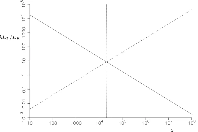
λET/EK
λ
Figure 4.Graphs of the ratioλET(0)/EK(0) (solid line) andλET(t1)/EK(t1) att1= 0.2 (dashed line) forRa= 3000 andα= 3.117. Also shown is the dotted line indicatingλ= 20994.
the exponential growth rate obtained from traditional linear analysis. The first method is to look at the ratio of the kinetic energy,EK(t), and temperature contributions,λET(t),
to E(t). For exponential growth this ratio will remain constant. In figure 4 are plotted the ratios ofλET(t) toEK(t) at the start and end of a time interval as functions ofλfor
[image:11.595.104.437.379.600.2]λ
E(t)
t
(a) (b)
Figure 5. Graphs showing (a) the estimated growth rate of the instabilities, ln(E(t1))/(2(t1−t0)) as a function of λ with t1 = 0.2., and (b) the evolution of E(t) for
λ= 100000 (dashed line),λ= 1000 (dotted) andλ= 20993 (solid line) for the caseRa= 3000,
α= 3.117,t0= 0 andt1= 0.1. Also shown in (a) is the dotted line indicatingλ= 20994.
The two lines cross at λ= 20994 where the ratios are the same at the start and end of the time interval.
The second approach for selecting λ is to look at the estimated growth rates of the disturbances based on the growth of the disturbances using
ln (E(t1))
2(t1−t0). (3.3)
Again using Ra = 3000 and α = 3.117 as a typical example, we get results shown in figure 5(a) showing the estimated growth rate as a function ofλ. This graph has a clearly defined minimum which is located atλ= 20994, the same point as found by the crossing lines in figure 4. If we look at the evolution ofE(t) fromt0= 0 tot1= 0.1 for the same example but with different values of λthen we get results as shown in figure 5(b). For
λ= 20994 the growth is a straight line on this logarithmic plot, indicating exponential growth which is at the growth rate expected from conventional linear stability analysis. For all other values ofλthere is an initial phase of faster growth before the growth of the instability settles down to the same exponential rate. Unless λ is chosen appropriately the growth rate is always overestimated if the average growth fromt0tot1is used. Some of the features we have seen here can be clarified by considering a simple model presented in the Appendix.
We have seen that unless we choose the parameterλappropriately we get an overesti-mate of the growth rate of the fastest growing mode for the Rayleigh–B´enard problem. We identified two possible selection procedures that yield the expected exponential growth rate for a heated layer:
• equate the ratio of the contribution toE(t) fromEK(t) andλET(t) att0and t1.
• minimize the optimal growth rate.
These approaches will give the expected exponential growth rate even if the total growth of the instabilities is only a few percent, and the time interval [t0, t1] lies in the period of the initial adjustments before the disturbance settles down to the exponential growth, seen at the left end of figure 5(b).
matrixAis
A=
λB 0
0 C
(3.4)
whereB andC are symmetric matrices. For generalΨ(t) we have
ET(t) =ΨT
B
0 0 0
Ψ and EK(t) =ΨT
0 0 0 C
Ψ. (3.5) We observe that
∂E(t)
∂λ =ET(t) + 2Ψ
TA∂Ψ
∂λ. (3.6)
Our optimised solutions satisfy (2.14). Differentiating with respect toλgives
MT
B
0 0 0
MΨ+MTAM∂Ψ
∂λ =
∂µ
∂λAΨ+µ
B
0 0 0
Ψ+µA∂Ψ
∂λ. (3.7)
If we pre-multiply this byΨTand substitute in (3.6) evaluated at bothΨ(t0) andΨ(t1) =
MΨ(t0) we find (after some manipulation)
∂E(t1)
∂λ =ET(t1)−E(t1)ET(t0). (3.8)
We have used here that E(t0) = 1 and so is independent of λ. It is straightforward to show that the statement λET(t0)/EK(t0) = λET(t1)/EK(t1) is equivalent to the right side of (3.8) being zero. Hence the ratio test and the minimum growth-rate criteria are equivalent for more generalM representing the evolution of disturbances other than just
exponential growth. This analysis assumes that the growthE(t) has a smooth minimum asλvaries. However, we will see later that in some cases the derivative at the minimum can be undefined, and the above result may not hold (see figure 12(b)).
Using the above criteria for selectingλit is found that it depends onRa,σandα. No simple relationship has been found between these variables, except for the special case of marginal stability at the critical wavenumber where
λ=σRa. (3.9)
This can be derived from the energy stability analysis of Joseph (1965, 1968) where he showed that, for this choice of λ, E(t) would decay for Ra less than the critical value required for linear instability, even if the disturbances were nonlinear.
Although we have identified two equivalent ways of selectingλthat give what may be considered the “correct” answer for the Rayleigh–B´enard problem, this may not be the appropriate choice in all circumstances. In real-world problems it may be that ambient disturbances to the velocity and temperature that initiate the linear instabilities may have a different ratio to those of the exponentially growing disturbances. For example, a large amount of background vibration may boost the velocity disturbances, or poorly designed heating elements in an experiment may give rise to a temperature field that is not as close to the ideal linear gradient as one would like, effectively boosting the temperature component. In these cases, imposing a restriction on the initial conditions and their contributions toEK(t) andET(t) would seem to be unphysical. However, the
In the above example the choices ofλwould seem to provide a relatively robust way of identifying instability. Both methods for making the choice ofλare numerically straight-forward. This will also be the case in the next section. However, there were found to be some cases for the problem of heating at a vertical sidewall where the presence of more than one unstable mode makes the selection criterion less straightforward. We will return to this later.
4. Heating semi-infinite fluid from a horizontal boundary
In this section we look at the stability of a semi-infinite fluid heated from below at a horizontal boundary. We restrict ourselves to the case where the dimensional wall temperature is assumed to instantaneously rise by ∆T at the initial time t = 0. The nondimensional background state for a boundary atz= 0 is
U(x, t) =0, T(x, t) =T0/∆T+ erfc
z
2t1/2
, (4.1)
where erfc(x) is the complementary error function. This is independent of the length-scale in the nondimensionalization, although we used (2.5). The boundary conditions are
u=0, T = 0 on z= 0, and u→0, T →0 as z→ ∞. (4.2)
One approach to evolving background states that has been used is to apply a quasi-static analysis. This assumes that the evolution of the background state can be ignored and an instantaneous stability analysis carried out. We include the results of such an analysis here for the purpose of comparison with later results which do not make this assumption.
In the quasi-static or frozen-time analysis we assume the background temperature pro-file is steady, i.e., the dimensionaltin the temperature profile is taken to be a parameter, saytq, and we use the length-scaleH= (κtq)1/2. This makes the nondimensionaltq= 1.
The stability of this will then depend on the value of the Rayleigh number. A linear stability analysis of this profile tells us that the thermal layer is unstable for a no-slip boundary when
Ra=gα∆T H 3
νκ =
gα∆T(κtq)3/2
νκ >
√
π. (4.3)
It should be noted that the critical value ofRa=π1/2(Kerr 2016) is around a thousand times smaller that the corresponding critical Rayleigh number for the Rayleigh–B´enard problem for a layer with two boundaries separated by a distance H = (κtq)1/2. The
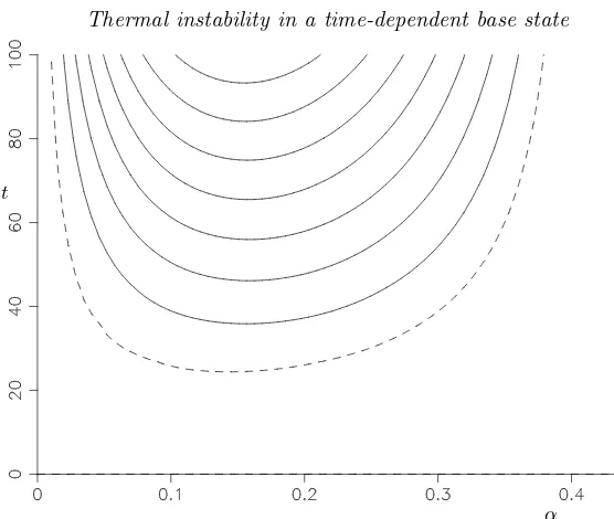
stability boundary of the critical value of Ra as a function of the wavenumber, α, is shown in figure 6(a). This does not depend on the Prandtl number,σ. Also shown in this figure are the contours of the growth rate for unstable modes forσ= 7. These curves are dependent on the Prandtl number. This instability is a long-wave instability, with the growth rate proportional toα2for smallαfor a givenRa.
If we use the alternative formulation whereRa = 1, then instead of looking for a critical value of Ra we look for the critical value of the nondimensional time tq to instability.
This gives the alternative, but equivalent, stability diagram shown in figure 6(b). Now the onset of instability is attq =π1/3. It should be noted that in both cases the rise in
the growth rates as Ra or tq increases is relatively slow. Although under this analysis
instabilities may start growing for moderate values of, say,tq such as those shown in the
Ra
α
Stable
tq
α
Stable
[image:15.595.94.470.104.264.2](a) (b)
Figure 6.Stability boundary showing the critical value of (a)Ra withtq = 1 and (b) tq with Ra= 1 under the quasi-static assumption withσ= 7. Also shown in both cases are growth rate contours with intervals of 0.02.
z
x
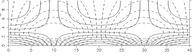
Figure 7.Contour plots of the instabilities showing the vorticity (solid lines) and temperature perturbation (dashed lines) for marginal stability forα= 0.15708.
other problems, if the transition from a stable regime to a fast-growing unstable regime is reasonably quick then the quasi-static assumption could give a good indication of when the onset of instabilities will occur.
Typical marginally-stable solutions found on the quasi-static stability boundary are shown in figure 7. The structure of the instabilities is split into two parts: a boundary layer of thickness of the order of the depth of temperature penetration that drives the instabilities, and an external region of size of order of the wavelength of the instabilities where the fluid adjusts in response to the convection in the boundary layer. This general structure applies to all the instabilities in a semi-infinite fluid heated from below that will be covered in this section, and not just those found using the quasi-static assumption.
In the study of the stability of the time-dependent thermal boundary layer, Foster (1965, 1968) used a truncated orthonormal function expansion inz for the temperature and vertical velocity. He fixed the initial condition which consisted of a vertical velocity perturbation. His tests revealed that varying this initial condition had little effect on the results. He then monitored the change in the kinetic energy. He used the natural length scaleL given by (2.5). We first mimic Foster by fixing t0 = 0 and only allowing initial conditions that are perturbations of the initial velocity, and look to maximise growth of kinetic energy. We can then find the earliest time t1 for instabilities to have grown so that their kinetic energyEK(t1)/EK(0) has grown by some predetermined factor. The
[image:15.595.130.442.313.404.2]t
[image:16.595.139.417.102.337.2]α
Figure 8.Graphs of the earliest times for the kinetic energy,EK(t), to have grown by a factor of 102
, 104 , 106
,. . .witht0= 0 (solid lines) as functions of the wavenumber,α, forσ= 7 and with initial perturbations restricted to the vorticity. Also shown is the time taken for the kinetic energy to first get back to its original level (dashed line).
time taken for the energy of the instabilities to return to their original levels (dashed line).
For larger times than shown in figure 8 all the contours converge towards the axis at
α= 0. However, by this stage the growth in amplitude of the instabilities will be very large, and assumptions of linearity are likely to have broken down.
If we now optimizeE(t1), while still retainingt0 = 0, then the picture is altered. We now have to select an appropriate value of λ. We can use either of the two equivalent methods for selecting this value in the previous section: ensuring the ratio of the contri-butions of the kinetic energy and the temperature toE(t) are the same at the start and at the finish, or minimizing the optimized growth as both are equivalent here. The results are as shown in figure 9. One notable difference between these results and the Foster case shown in figure 8 is that the dashed line, which indicates the time taken forE(t) to get back to its initial value is significantly lower. This is more in line with the quasi-static analysis which showed the existence of slowly growing solutions for quite small values oft. The initial dip in the kinetic energy when there was no initial temperature perturbation was noted in the Rayleigh–B´enard case, but it is exacerbated here by the absence of a vertical background temperature gradient whent= 0. The need for this gradient to de-velop further delays the creation of the temperature perturbation. However, for the cases shown in figure 9 there is an initial temperature perturbation appropriate for a growing instability. This slows down the reduction in the kinetic energy, and all that is required is for the background temperature gradient to develop sufficiently for instabilities to grow. As we saw from the quasi-static analysis the time when appropriate disturbances can start growing can be in the low single figures, which is compatible with the results seen in figure 9. For later times the growth in E(t) is more that 100 times larger than the corresponding growth in the Foster case.
t
[image:17.595.118.431.101.338.2]α
Figure 9.Plots of the earliest time forE(t) to have grown by a factor of 102 , 104
, 106
,. . .with
t0= 0 (solid lines) as functions of the wavenumber,α, forσ= 7 withλoptimized. Also shown are the times taken forE(t) to get back to its original level (dashed line).
t
α
Figure 10. The optimal value of t1 (solid lines) as a function ofα for E(t1)/E(t0) = 10 2
, 104
, 106
and 108
, along with the corresponding value of t0 forE(t1) = 10 2
(dotted line). For comparison, the corresponding optimal values oft1 witht0 = 0 are also shown (dashed lines). These are forσ= 7 withλoptimized.
[image:17.595.137.432.387.609.2]t1
σ
α
σ
[image:18.595.96.474.106.264.2](a) (b)
Figure 11. Plots for t0 = 0 showing the dependency on the Prandtl number of (a) time for instabilities to grow,t1, and (b) the wavenumber,α, forE(t1) = 100,10
4
, 106
,108
(from bottom to top in (a), and top to bottom in (b) at the left end). Also shown are the small and large Prandtl number asymptotics (dashed lines) forE(t1) = 10
4
and 108
. In all cases the optimal value ofλis used.
curves only diverge towards the right hand end. At the low point of each curve, where the globally optimal instabilities are to be found, the curves are almost indistinguishable. The left hand end of these graphs have low values of the wavenumbers, and the natural dissipation rate for these modes, which have a significant proportion of the disturbances outside the thermal boundary layers, is small. As such, an initial condition imposed at
t= 0 will change little before instability sets in.
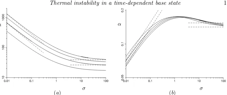
All the above results presented so far have been for Prandtl number σ = 7, a value appropriate for, say, water. Looking at a range of Prandtl numbers we find the minimum time for the growth of instabilities,t1, varies as shown in figure 11(a) for the caset0= 0. These show that for large Prandtl numbers the time taken to the onset of instabilities levels off, while for small Prandtl numbers the slopes of the curves tend towards −2/3 and so the time to instability grows with t1∝σ−2/3. The wavenumbers,α, decrease as
σ1/3 for small Prandtl numbers. For large Prandtl numbers the picture is not as clear, but there is an apparent levelling off of the curves.
For the low Prandtl number limit the viscous dissipation term becomes insignificant in comparison to the inertia terms. If we neglect the∇2ω term, and use the rescalings
t=σ−2/3t′
, x=σ−1/3x′
, ω=σ−2/3ω′
, ψ=ψ′
, T =T′
, (4.4)
then the governing equations reduce to
∂ω′ ∂t′ =
∂T′
∂x′, (4.5a)
∂2
∂x′2 +
∂2
∂z′2
ψ′
=−ω′
, (4.5b)
∂T′ ∂t′ −
e−(z′)2/4t′ (πt′)1/2 w
′
=
∂2
∂x′2+
∂2
∂z′2
T′
. (4.5c)
These equations are now independent of the Prandtl number. This rescaling removes the dependency on the viscosity,ν, that was present in the original length scaling (2.5). These equations can be solved in a similar way to the previous set of equations, with optimisation for λ as before. For example, with t0 = 0 and E(t1) = 104 the optimum wavenumber is found to beα′
= 0.3353 andt′
asymp-totic predictionsα= 0.3353σ1/3 andt
1= 29.94σ−2/3 shown in figure 11, along with the corresponding low Prandtl number asymptotics forE(t1) = 108.
For the high Prandtl number limit the inertial term becomes insignificant, with the fluid motion being a balance between the buoyancy forces and the viscous dissipation. With the inertia term neglected, σ no longer appears in the governing equations, and so the instabilities do not depend on the Prandtl number at leading order. The gov-erning equations now have the vorticity being dependent directly on the instantaneous temperature, and so we only optimise over all possible initial conditions for the temper-ature. Otherwise the method is essentially the same as before. For example, witht0= 0 and with E(t1) = 104, the optimum t1 and corresponding wave number are given by
t1 = 26.30 and α= 0.1543. These asymptotes are shown to the right of the graphs in figure 11 along with the corresponding lines forE(t1) = 108. The asymptotics fort1show good agreement, however those forαare not as convincing.
If one also includes optimisation for t0 then these curves and asymptotics are little changed. The low Prandtl number asymptotics indeed have t0 = 0. There is no viscous dissipation, and the instantaneous Rayleigh number becomes infinite as soon as the heating starts. However, the instabilities still take a finite time to grow. For the large Prandtl number asymptotics we find t1 to be weakly dependent on t0, with a small decrease int1of around 0.6% for E(t1) = 104 whent0= 2.60.
In this section we have investigated the optimal time for instabilities to grow for a semi-infinite fluid heated from below by a sudden increase in the temperature at the boundary. Because the initial state allows perturbations to both the vorticity and the temperature, the onset of instability is sooner than that found by Foster and the overall growth is subsequently significantly larger. Allowing the instabilities to start at some time after the onset of heating did not, unfortunately, have a significant impact with, at best, only a marginal decrease in the time for a given growth of the instabilities.
5. Heating a semi-infinite fluid from a vertical boundary
In this section we look at the instabilities that can form at a heated vertical boundary. For a semi-infinite fluid the heat diffuses into the fluid just as for the horizontal boundary, but now the buoyant boundary layer induces an upwards flow parallel to the wall. The nondimensional vertical flow and temperature profiles are given by (forσ6= 1)
U(x, t) =W(x, t)ˆz= σ (1−σ)
t+x 2
2
erfc x 2t1/2
−xt
1/2
π1/2 exp
−x 2 4t , −
t+x 2 2σ erfc x
2(σt)1/2
+ xt 1/2
(σπ)1/2exp
−x 2 4σt ˆ
z, (5.1a)
T(x, t) =T0/∆T+ erfc
x
2t1/2
. (5.1b)
The appropriate boundary conditions for the perturbations are
u=0, T = 0 on x= 0, and u→0, T →0 as x→ ∞. (5.2)
Here we have used the natural scaling (2.5) in the nondimensionalization. For lateral heating in a vertical slot of widthH the Grashof number, given by
Gr= gα∆T H 3
ν2 , (5.3)
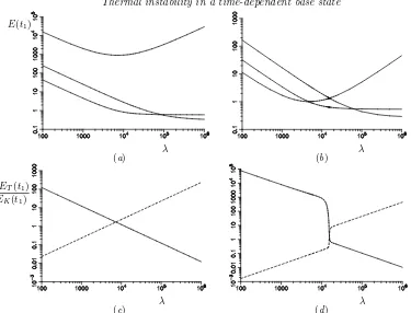
length-E(t1)
λ λ
(a) (b)
λET(t1)
EK(t1)
λ λ
[image:20.595.86.461.109.395.2](c) (d)
Figure 12.Graphs of the growthE(t1) as functions ofλfor the three most unstable modes for
σ= 7, t0 = 0, andt1 = 160.with (a) α= 0.030 and (b) α= 0.035. The corresponding ratios
λET(0)/EK(0) (solid lines) andλET(t1)/EK(t1) (dashed lines) for the most unstable mode are shown in (c) and (d) respectively.
scale by using the length H that makes this unity. This would result in an alternative length scale that differs from the length-scale (2.5) by a factor ofσ1/3, with corresponding changes to other scalings used in the nondimensionalization. However, we will retain our previous definition ofLto maintain compatibility between the problems considered here. The governing equations for linear disturbances are solved in a similar numerical way to those of the previous section but with two main differences. Because there is a background flow along the wall, we no longer have stationary instabilities and have to calculate both the real and imaginary parts ofω,ψ andT.
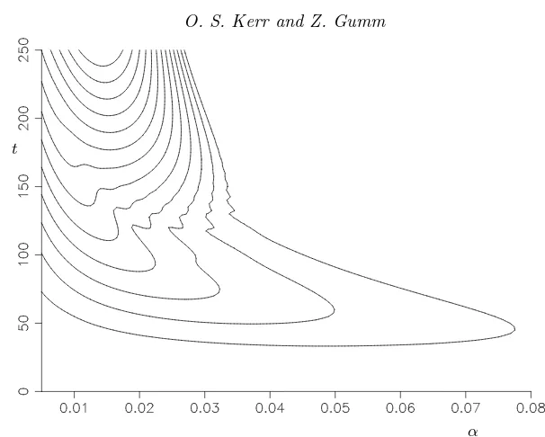
t
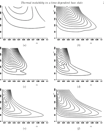
[image:21.595.129.432.99.342.2]α
Figure 13.Growth in energy of instabilities, withσ= 7. Contours atE(t1) = 10, 100, 1000,
. . .witht0= 0.
defined minimum, it is no longer as smooth, but has a discontinuity in its derivative at its lowest point. The lines forλET(0)/EK(0) andλET(t1)/EK(t1) in figure 12(d) still cross over near the minimum of the growth rate, but the apparent continuity of these curves, although rapidly changing near the crossover, would appear to be due to numerical effects in the eigenvalue solver which results in a degree of smoothing in what one would expect to be curves with discontinuities.
When the same mode is the most unstable for all values ofλthen the selection of the appropriate value is straightforward. When we have the more complex picture then we can still choose the value ofλcorresponding to the minimum of the maximized growth in energy. At such a point there is a degree of degeneracy in the problem, and the eigenvector from (2.14) is no longer uniquely defined. It would be possible to look at each eigenmode individually and find its minimum growth rate, or point where the initial and final energy ratios are the same. However, this does not necessarily make much sense physically as for any such choice ofλthe most unstable mode will not be one that is identified by such an approach.
The above argument would seem to indicate that the most appropriate method of choosingλis to select the value corresponding to the minimum growth. However, this is not without some practical difficulties. As can be seen towards the right of figures 12(a) and (b), some modes have very flat sections in their growth. The value ofλfor minimum growth for such modes can be relatively hard to identify numerically. Problematic cases were only found for modes that did not grow significantly, or which had grown and then subsequently reduced in magnitude, and are not relevant to the main results presented here.
t
α
t
α
(a) (b)
t
α
t
α
(c) (d)
t
α
t
α
[image:22.595.105.472.101.562.2](e) (f)
Figure 14.Growth inE(t) of instabilities for (a) σ= 0.1, (b)σ= 1, (c)σ= 3, (d) σ= 7, (e)
σ= 10 and (f)σ= 20 as functions of α. The contours are forE(t1) = 10, 100, 1000, . . . with
t0= 0.
t1
σ
α
σ
[image:23.595.93.472.102.265.2](a) (b)
Figure 15.Plots showing the dependency on the Prandtl number of (a) time for instabilities to grow,t1, and (b) the wavenumber,α, forE(t1) = 100, 10
4
, 106
, 108
(from bottom to top in (a), and top to bottom in (b) at both ends) fort0= 0.
number mode for larger times than is shown here. However, as E(t1)> 1013 it is not clear that this linear analysis will be relevant in practical problems as nonlinear effects are likely to be important by this stage.
It is the presence of the two modes that can be used to explain the wiggles in the contours observed in figure 13 and in some of the examples in figure 14. If two differ-ent modes are presdiffer-ent they will typically move upwards at differdiffer-ent rates. For given amplitudes of the modes we would expect that in some alignments the value ofE(t) is enhanced and in some alignments it will be decreased. For some time intervals, [t0, t1], it is possible for the modes to start off in an alignment that diminishesE(t), and end up in an alignment that enhances it. This will result in some boost in the apparent growth. For other time intervals the modes would start and finish with eitherE(t) enhanced at botht0 andt1, or diminished. In these cases there would not be such an apparent boost to the growth. Hence in the region where neither mode dominates one could expect there to be the possibility of some variability in the growth ofE(t) due to the variation in the length of the time interval [t0, t1], in addition to that caused by the underlying growth of the instabilities. This effect is shown by the wiggly contours.
The most unstable modes, where a given growth in E(t) is attained soonest for the caset0= 0, are given by the minimum of these curves. If we look at the effect of varying the Prandtl number on the most unstable modes for growths of E(t) by factors of 102, 104, 106 and 108 then we obtain the results shown in figure 15. The general trends are similar to those for heating from a lower boundary found in the previous section. The most unstable modes have a transition due to the appearance of the large Prandtl number mode. There is a transition indicated by the kinks in the curves fort1forE(t1) = 104, 106 and 108 where the minimum associated with the large Prandtl number mode takes over as the global minimum. This is shown by the corresponding jumps in the wavenumbers,
α. In both the limits of large and small Prandtl numbers the approaches that yielded the asymptotics for the bottom heating cases did not yield results as readily. It seems that the shear is important to these instabilities. The analysis of shear driven instabilities is more complicated (see, for example, Drazin & Reid 1981) and is beyond the scope of this paper.
t1
t0
E(t)
t
[image:24.595.99.476.104.266.2](a) (b)
Figure 16.In (a) is shown the graph of the optimal value of the end time,t1, as a function of the start time,t0, for growthE(t1) = 10
4
, withα= 0.02106 andσ= 7. In (b) the evolution of
E(t) for the examples with t0 = 0 and the global minimum of (a) (solid lines). Also shown is the growth corresponding to the minimum of the main curve (dashed line).
σ= 7. This choice ofαcorresponds to the overall optimal instability forE(t1) = 104, as we shall see later. The overall minimum value oft1is found at the bottom of the isolated loop at the left of this plot. The maximum of this loop and the overall minimum of the main line both have a role in the overall stability boundary. When we vary α we find that the loop observed in figure 16(a) merges with the main line for smaller values ofα, while asαincreases this loop shrinks and vanishes. Not shown here is that the main line in (a) continues to rise and then doubles back on itself to form a larger loop that rejoins the axis to the left at much higher values oft1, and so the optimised solution eventually decays withE(t)<104 for this value ofα.
The evolution of E(t) for the mode with the overall minimum value of t1 and the optimal mode witht0= 0 are shown by the two solid lines of figure 16(b). These cross over after a short time and then grow approximately in parallel, showing the optimal solution which starts at a slightly later time avoids a brief period of decay and an initial period of more sluggish growth experienced whent0= 0. The dashed curve in (b) represents the growth of the mode corresponding to the first minimum of the upper branch in (a). In the evolution of this mode,E(t) exceeds 104 before undergoing a short period of decay, dropping to below the threshold level and then rising again. It can be observed that this dashed line reaches the level of 104fractionally before the optimal value. This is because the value of λis optimised for each mode, and the two cases will have different values. When λ is optimised for the overall minimum growth, other values of λ will result in apparently faster growing modes.
The variation withαof the values oft1at the maximums and minimums of the curves in figure 16(a) are shown in figure 17(a). The corresponding values of t0 are shown in figure 17(b). The dotted lines indicates α= 0.02106, the overall minimum of the curves in figure 17(a). This is the value used for the results in figure 16. The main line in (a) cuts the dotted line three times. These correspond to the two minimums and the maximum at the left of figure 16(a). The S-shaped nature of the curve as it passes through the points corresponds to the joining of the isolated loop with the main branch of solutions for lower
t1
α
t0
α
[image:25.595.97.472.105.263.2](a) (b)
Figure 17.The location of the maximums and minimums of thet0–t1 plots as functions ofα forE(t1) = 10
4
, withσ= 7 are shown in (a). The corresponding values oft0 are shown in (b). The vertical dotted line showsα= 0.02106, the value used in figure 16.
t1
α
Figure 18.The minimum time, t1, of the first instabilities to grow by factors of 10, 102 ,. . ., 108
as functions ofα(solid lines) when the initial time,t0, is optimised for σ= 7. The dashed show the corresponding curves whent0= 0.
right end of the main curve in figure 17 no optimised instabilities haveE(t) that reach 104.
[image:25.595.125.443.308.535.2]Figure 19.The evolution of the vorticity perturbations (top) and temperature perturbations (bottom) for the most mode with the earliest growthE(t1) = 104
, forα= 0.02106 forσ = 7. At the left are the initial conditions att0 = 11.52 and the right the evolved instabilities at
t1= 83.42 with the intermediate steps show at equal time intervals.
is the only section of these curves where the minimum in the maximum growth asλ is varied is not a simple minimum, but corresponds to a change in the most unstable mode similar to the case illustrated in figure 12(b).
The form of the instabilities is different for the small and large Prandtl number modes. The evolution of the instabilities betweent0andt1for the lowest value oft1withE(t1) = 104andσ= 7 is shown in figure 19. This case lies entirely within the large Prandtl number regime. The temperature perturbation settles down to an arrowhead shape centred on the centre of the background upwards flow.
Figure 20.The evolution of the vorticity perturbations (top) and temperature perturbations (bottom) for the most mode with the earliest growthE(t1) = 104
, forα= 0.01503 andσ= 7. At the left are the initial conditions att=t0= 14.17 and the right the evolved instabilities at
t=t1= 171.34 with the intermediate steps show at equal time intervals.
point corresponds to the transition from the region of instability associated with high Prandtl number to that associated with low Prandtl number identified in figure 14. The maximum vorticity perturbation is now closer to the wall in the region of greatest shear. The temperature perturbation no longer has a maximum near the location of the maximum upwards velocity, but has a wider shape, with maxima on either side of the maximum up-flow.
E(t)
t
E(t)
t
[image:28.595.88.475.107.258.2](a) (b)
Figure 21. Growth inE(t) of optimised instabilities with E(t0) = 1 fort betweent0 andt1 for (a)E(t1) = 104
and (b)E(t1) = 10 8
. Also shown are the contributions to these fromEK(t) (dashed line) andλET(t) (chained line). These haveσ= 7.
in the plots of the contribution to E(t) from EK(t) and λET(t) shown in figure 21 for
the above two cases. For the case where E(t1) = 104 most of the contribution to E(t) comes from the temperature component. The instabilities are centred on the region of maximum upwards velocity in the background flow — the region of least shear. This is also true in the first part of the case withE(t1) = 108. HereE(t) grows until it reaches a local maximum at a level that is in line with maximums observed in the evolution of the large Prandtl number modes. There is then a transition to a new mode whereEK(t)
andλET(t) are much closer in size.
In the above examples, although the initial growth rate ofE(t) is reasonably constant, there are signs of small adjustments inEK(t) andλET(t) similar to those observed when λwas not optimal for the Rayleigh–B´enard case. One possible explanation of this is that the selection method forλensures that the ratiosET(t0)/EK(t0) andET(t1)/EK(t1) are identical. This ratio is determined at the end primarily by the fastest growing mode, and so the initial conditions have to satisfy a constraint that may not match up to the ratio in the initial mode of growth. The mismatch is greater in the E(t1) = 108 case where the initial and final growth modes are clearly different. In addition the optimal initial conditions found for both cases do not resemble the instabilities once they have evolved. The initial conditions have a slope that is the opposite direction to that which you get when the shear acts on the instabilities, and which is observed for the later stages of their evolution. This could allow the instabilities to have an initial stage of boosted growth before shear starts to have a limiting effect.
The results of simulations with random noise shown in figure 1 correspond to the calculations shown in figure 21(b), using the same vales of α and λ. The simulations were subject to random noise being added to the temperature perturbation throughout the run, which started at t = −160 to allow the perturbations to settle down to an approximate statistically-steady state before the heating of the wall starts. The general growth of the randomly-driven simulations in the last half of the time interval shown are clearly similar to the growth shown in figure 21(b) for nearly all cases. However details of the onset of instability, and of the size of the growth are hidden by the random noise in the first half of the interval.
t
E(t1)
α
E(t1)
[image:29.595.94.478.105.272.2](a) (b)
Figure 22.Graphs of (a)t1 (upper curves) andt0 (lower curves) and (b)αfor the fully optimized solutions as functions ofE(t1) forσ= 7.
the large Prandtl number modes, while for larger values it is the minimum of the small Prandtl number mode. In the transition region there are at least two minimums, with the values corresponding to the continuations of the global minimums shown here. The presence of the wiggles leads to other short-lived minimums which are not significant in the overall dynamics. Clearly visible in this plot is the transition between the two modes of instability, with the relatively slow growing large Prandtl number mode giving way to the faster growing small Prandtl number modes for larger growths.
One feature of interest is that for both the large and small Prandtl number branches the relationship betweent1andE(t1) is approximately linear on these graphs, indicating no significant change in the growth rates once the instabilities are established. This is despite the fact that the temperature profile and the background flow are evolving. Both the instantaneous Rayleigh number and Reynolds number grow ast3/2.
There is also a significant variation in the wavenumber for the most unstable modes as the growth increases for the initial large Prandtl number mode. However, there is relatively little variation once the small Prandtl number mode takes over, thus the in-stabilities that one may observe could have a relatively well defined wavelength.
In this section we have investigated the growth of instabilities in the evolving boundary-layer flow generated by the heating of a fluid at a vertical wall. In looking for the earliest growth of the size of the instabilities, as measured by E(t), we have shown that this growth can be advanced by delaying the imposition of the initial conditions. However, this enhancement is not huge for this problem.
6. Conclusions
the velocity and monitoring the growth of the kinetic energy can lead to an underestimate in the growth by an order of magnitude. Similarly using an inappropriate balance between the measure of the contribution from the kinetic energy and from the temperature can lead to exaggerated growth, or even apparent instability when none is really there.
The instabilities when a body of fluid is heated from below start to grow far sooner than one might expect based on an estimate of the instantaneous Rayleigh number and comparison with the Rayleigh–B´enard problem. The instabilities have a long wavelength when compared to the thickness of the buoyant thermal layer. The general behaviour of the instabilities changed continuously over a range of Prandtl numbers, and the large and small Prandtl number asymptotics were identified. The decay rate for disturbances of this size is relatively small, and so there is little, if any, significant decay before insta-bility starts. Over the range of Prandtl numbers optimising the initial time for start of instabilities had little or no effect.
When fluid is heated from a sidewall it was found that there were two instability modes corresponding to large and small Prandtl numbers. For intermediate Prandtl numbers such as that of water both modes played a role. For lower growths in the amplitude of the instabilities in this intermediate range the optimal instabilities were large Prandtl number modes. For larger growths the initial development of the optimal instabilities was as a large Prandtl number mode, before undergoing an transition to the small Prandtl number mode. The large Prandtl number modes were centred around the region of max-imum velocity of the buoyant up-flow caused by the heating, while the small Prandtl number modes had a more complex structure. For both modes the growth rate of the instabilities seems relatively constant even though the background state and the form of the instabilities were both evolving.
We have used the method for identifying the most unstable modes to look at the evolu-tion of linear disturbances to semi-infinite bodies of fluid in the two cases of heating from below at a horizontal boundary and heating from a vertical boundary. We have identi-fied these instabilities by finding the initial conditions that maximized the growth of a measure of the amplitude instabilities,E(t). For the bottom heating case the instabilities were stationary — they did not move along the wall. For the sidewall case the instabilities travelled upwards with the boundary layer flow. In other problems where the approach used here could be applied the instabilities may possibly be oscillatory in their nature. For example, one could look at the standing oscillatory double-diffusive convection observed when a layer of fluid with a stable salinity gradient is heated from below (Baines & Gill 1969), where the instabilities predicted could take the form of standing oscillatory insta-bilities or travelling waves of instability, or combination of the two. Although only one undetermined parameter was involved here in the measure of the amplitude of the distur-bances, for double-diffusive convection where there are contributions to the density from both temperature and salinity a minimum of two parameters would be required, say, by adding aµS2term to the integral in (2.8), whereS is the salinity perturbation. However, the energy stability analysis of Kerr (1990) required three parameters, the equivalent of addingµ(S−γT)2to the integral. This may be required if the current method is applied to double-diffusive problems. In the regimes where instabilities are oscillatory, unless the instability is purely a travelling wave, then the contributions of the velocity, temperature and, in this case, salinity toE(t) would have oscillatory components as the disturbance grew. For a standing instability the kinetic energy could regularly vanish even though the instability as a whole would be growing. It would be expected that with the appropriate choice of the measure of the amplitude these oscillations would not prove problematic.
However, the adjoint partial differential equations for this problem are neither derived, nor explicitly solved. For most of the problems looked at using the adjoint equations there has been no temperature component, and just looking at the kinetic energy of the perturbations would be an appropriate measure of the amplitude of the disturbances, and the results previously obtained should be the same as any found using the current approach.
In the problems looked at here the adjoint mapping A−1MTA
depends on the param-eterλ, through the matricesA−1 andA. The bulk of the calculations are spent finding,
M, which is independent of the measure of the amplitude. So varying λto optimise the
growth for givent0 andt1is a relatively quick step.
The choice of expressing the solutions as a simple vector (2.10) and the numerical approach used here for obtaining the matricesM was primarily chosen for simplicity. It
would also be possible to use other methods such as using functional expansions for the temperature and vorticity. These will alter the details of the various matrices involved, but not the overall method. The same approach for finding optimal solutions could be applied to these more advanced numerical methods.
Although optimizing for the start time for the instabilities, t0, was almost entirely unimportant for the heating of a semi-infinite body of fluid from below, it had a small effect when the boundary was vertical. For other problems where there may be a signifi-cant delay before the onset of instabilities, it could be important. As we have mentioned in the introduction there are some convection problems where there was a significant period between the onset of heating and the observation of instabilities.
We would like to acknowledge the financial support provided to Z. Gumm by The School of Engineering and Mathematical Sciences, City University London.
Appendix
Here we present a simple model to help explain the variations ofE(t) =EK(t)+λET(t)
for the most unstable modes as λis varied as seen in figure 5(a). We will consider a 2 component analogue. Over a time interval fromt0 tot1 and initial state (1, a) grows by a factor ofGtoG(1, a), while a second mode (1, b) decays to zero. We also require that
ab <0. If we consider the first component of these vectors to correspond to the velocity and the second to the temperature then the initial “energy” of a general disturbance
A(1, a) +B(1, b) will be
E0= 1 4
(A+B)2+λ(Aa+Bb)2
. (A 1)
The final energy will be
E1= 1 4
G2A2(1 +λa2)
, (A 2)
and so the growth in the energy is
E1/E0=
G2A2(1 +λa2) (A+B)2+λ(Aa+Bb)2 =
G2(1 +λa2)
(R+ 1)2+λ(Rb+a)2, (A 3)
where R = B/A. For a given λ we want to find R that maximizes this growth. This occurs when