Experimental and numerical investigation of a double concentric bluff body flameholder

Rochester Institute of Technology

RIT Scholar Works

Theses

Thesis/Dissertation Collections

8-1-1995

Experimental and numerical investigation of a

double concentric bluff body flameholder

Peter Eliot Zeender

Follow this and additional works at:

http://scholarworks.rit.edu/theses

This Thesis is brought to you for free and open access by the Thesis/Dissertation Collections at RIT Scholar Works. It has been accepted for inclusion

in Theses by an authorized administrator of RIT Scholar Works. For more information, please contact

ritscholarworks@rit.edu.

Recommended Citation

"Experimental and Numerical Investigation of a Double Concentric

Bluff Body Flameholder"

by

Peter Eliot Zeender

A Thesis Submitted

In

Partial Fulfillment

of the

Requirements for the

MASTER OF SCIENCE

ill

Mechanical Engineering

Approved by:

Professor:

Satish Kanlikar

(Thesis Advisor)

Professor:

_

(Dr.

Alan

Nye)

Professor:

-(Dr.

Ali

Ogut)

Professor:

-(Deptartment Head)

DEPARTMENT OF MECHANICAL ENGINEERING

COLLEGE OF ENGINEERING

AUGUST 1995

PERMISSION GRANTED:

I, Peter Eliot Zeender, do hereby grant permission to the Wallace Memorial Library of the

Rochester Institute of Technology to reproduce this thesis entitled "Experimental and

Numerical Investigation of a Double Concentric Bluff Body Flameholder" in whole or in

part, for educational use only.

December 15th, 1995

Peter Eliot Zeender

FORWARD:

This

work

has been

almost

two

years

in

the

making,

and

it has

proved

to

be

the

academic

highpoint

of

my

engineering

career.

The

list

of people

I

would

like

to thank

for

all

their

help,

inspiration,

support

and

understanding

is

too

enormous

to

put

to

pen.

I

would

like

to

make special note of a

few though,

as

this

work would

be incomplete

without

their

mention.

I

would

like

to

thank

Dr.

Kandlikar,

for

putting up

withme

for

so

long. He has

been instrumental in maintaining

an academic environment

that

makeswork such as

this

posssible.

His

endless

support and guidance are

greatly

appreciated.

I

would

like

to thank

Dr.

Ogut

and

Dr. Nye

for

aiding

me

in putting

this

work

into

its

final

presentable

form. I

extend great appreciation

to the

RIT Machine

Shop,

especially Dave

Hathaway,

Jim

Greanier

and

Tom

Locke for

everything

they

have

done for

me.

I

want

to

extend a special

thanks to

Janet

Zandy,

for

directing

my

vision

to

the

concerns of

the

world outsideof

engineering,

a gift

that

has helped

to

change

my life.

I

want

to

extend

my

love

and

thanks to

all of

my

family; Mom, Dad, Aaron,

Nathan,

the

fam,

Grandma

and

Grandpa

for

giving

me

the

support

I

needed

to

bring

this

work

to

fruition.

A very

special

thanks to

my

best friend

Tracy

Avgerinos

for

more

than

I

can put

into

words.

Thanks

to

all

my

academic peers and

friends,

who

have

played such a vital role

in

my

life

these

past

five

years.

And

lastly,

though

by

no means

the

least,

my

thanks to

Dr.

Abdel

Hafez,

a mentor without whom

this

work could never

have

been

concieved.

It

was

hisguidance

and

friendship

that

put me on

the

path

I

am

today,

I

for

that

I

am grateful.

ABSTRACT:

In

the

present

investigation,

the

flow

through

a

double

concentric

bluff

body

flameholder is

examined.

The

flameholder

is

studied

numerically,

using commercially

available

computational

dynamics

software

CFDS-Flow3D;

and

experimentally,

using

a

burner

test

stand

constructed

for

the

study.

The

capabilities of

the

software are

first

validated

by

anumerical recreation of

experimental work

done

by Huang

and

Lin

(1994)

on a single

bluff

body

flameholder. This

work

is

then

extended

by

converting

the

numerical models

to

include

a propane

jet,

serving

as a reference

for

the

double

bluff

body

models.

The

flameholder is

numerically

modeled under

both

cold

flow

andcombustion

conditions

for

a propane

diffusion

flame,

for four

separate conditions of operation.

An

experimental analysis

is

also conducted with

the test

stand

to

verify

the

results of

the

numerical combustionmodel.

The

numericalresults

for

the

flame

shape and envelope

agreed

closely

with

the

experimental

data.

VI 1

XI

TABLE OF

CONTENTS:

List

of

Figures

List

of

Tables

Nomenclature

1.0

Introduction

1

2.0

Objectives

3

3.0

Literature

Search

4

3

.

1

Principles

of

Combustion

4

3.11

Chemistry

of

Combustion

4

3.12

Flames

6

3.13 Flame

Stabilization

8

3

.

2 Bluff

Body

Flameholders

1

0

3.3 Review

of

Single

Bluff

Body

Cold

Flow Analysis

13

4.0

Computational Fluid Dynamics Analysis Overview

1 7

4.

1

Operation

Principles

of

CFD

1 7

4

.

2 Numerical Model

for Single

Bluff

Body

21

4.3

Numerical

Model

for Double

Bluff

Body

-

Cold

Flow

26

4.4

Numerical

Model

for

Double Bluff

Body

-

Combustion

30

4.5

Output

from

the

CFD Code

3 5

5.0

Numerical

Validation Analysis

36

5

.

1

Cold

Flow Analysis

of

Single

Bluff

Body

36

6.0

Double Bluff

Body

Numerical

Analysis

60

6.1

Cold

Flow Analysis

60

6.2

Combustion

Analysis

78

7.0 Experimental

Analysis

96

7. 1

Experimental

Setup

96

7.2

Experimental

Procedure

100

7.3

Experimental Results

102

8.0

Conclusions

114

References

116

Appendices

A.

Sample CFD Command

Files

A-l.

Single

Bluff

Body

with

Propane

(Case

II

A)

A-2.

Double Bluff

Body

-

Cold

Flow (Case

Alpha)

A-3. Double Bluff

Body

-

Combustion

(Case

Alpha)

B.

Sample CFD Output File

LIST OF

FIGURES:

3.1

Standard

Diffusion Flame

Concentration

Profiles

7

3.2 Flow

Pattern

around various

Bluff

Bodies

1

1

3.3

Characteristic

Regions

of

Flow,

Huang

and

Lin

16

4. 1

Model

Outline

for Single

Bluff

Body

23

4.2

Boundary

Conditions

for Single

Bluff

Body

24

4.3

Grid Structure for

Single Bluff

Body

25

4.4 Model Outline

for

Double Bluff

Body

-

Cold Flow

27

4.5

Boundary

Conditions for Double

Bluff

Body

-

Cold

Flow

28

4.6

Grid Structure for Double

Bluff

Body

-

Cold

Flow

29

4.7

Model

Outline

for Double

Bluff

Body

-

Combustion

3 1

4.8

Boundary

Conditions for

Double Bluff

Body

-

Combustion

32

4.9

Grid Structure for

Double Bluff

Body

-

Combustion

33

4. 10

Grid Structure for Double

Bluff

Body

-Combustion,

Enhanced View

34

5. 1

Single

Bluff

Body,

Case

II

(A):

Velocity

Vectors

37

5.2

Single

BluffBody,

Case

H

(A):

Axial

(V) Velocity

Contours

38

5.3

Single

BluffBody,

Case

II

(B):

Velocity

Vectors

39

5.4

Single

BluffBody,

Case

II (B): Axial

(V) Velocity

Contours

40

5.4

Single

BluffBody,

Case

U

(C):

Velocity

Vectors

41

5.6

Single

BluffBody,

Case

II (C): Axial

(V) Velocity

Contours

42

5.7

Single

BluffBody,

Case

HI:

Velocity

Vectors

43

5.8 Single

BluffBody,

Case

IH: Axial

(V) Velocity

Contours

44

5.9

Single

BluffBody,

Case

IV

(B):

Velocity

Vectors

45

5.10

Single

BluffBody,

Case

IV (B): Axial

(V)

Velocity

Contours

46

5.11

Single

BluffBody,

Case

II (A):

Propane

Concentration

52

5.12

Single

BluffBody,

Case

II (B):

Propane

Concentration

53

5.13

Single

BluffBody,

Case

II (C):

Propane

Concentration

54

5.14

Single

BluffBody,

Case

III:

Propane Concentration

55

5.15

Single

BluffBody,

Case

IV

(B): Propane

Concentration

56

6. 1 Double

BluffBody

-

Cold

Flow,

Case

Alpha:

Velocity

Vectors

62

6.2

Double

BluffBody

-

Cold

Flow,

Case

Alpha: Axial

(V) Velocity

Contours

63

6.3

Double

BluffBody

-

Cold

Flow,

Case

Alpha: Propane Concentration

64

6.4

Double

BluffBody

-

Cold

Flow,

Case

Beta:

Velocity

Vectors

65

6.5

Double

BluffBody

-

Cold

Flow,

Case

Beta: Axial

(V) Velocity

Contours

66

6.6 Double

BluffBody

-

Cold

Flow,

Case

Beta: Propane Concentration

67

6.7

Double

BluffBody

-

Cold

Flow,

Case

Chi:

Velocity

Vectors

68

6.8

Double

BluffBody

-

Cold

Flow,

Case Chi:

Axial

(V) Velocity

Contours

69

6.9

Double

BluffBody

-

Cold

Flow,

Case

Chi: Propane Concentration

70

6. 1 0 Double

BluffBody

-

Cold

Flow,

Case

Delta:

Velocity

Vectors

7 1

6. 1 1

Double

BluffBody

-

Cold

Flow,

Case

Delta: Axial

(V) Velocity

Contours

72

6.

12

Double

BluffBody

-

Cold

Flow,

Case

Delta:

Propane Concentration

73

6. 1 3 Double

BluffBody

-Combustion,

Case

Alpha,

Temperature

Contours

8 1

6. 14 Double

BluffBody

-

Combustion,

Case

Alpha,

Products Concentration

82

6. 15

Double

BluffBody

-Combustion,

Case

Alpha,

Propane

Concentration

83

6. 16

Double

BluffBody

-Combustion,

Case

Beta,

Temperature Contours

84

6. 17

Double

BluffBody

-Combustion,

Case

Beta,

Products

Concentration

85

6. 18

Double

BluffBody

-Combustion,

Case

Beta,

Propane Concentration

86

6.19

Double

BluffBody

-Combustion,

Case

Chi,

Temperature Contours

87

6.20

Double

BluffBody

-Combustion,

Case

Chi,

Products Concentration

88

6.21

Double

BluffBody

-Combustion,

Case

Chi,

Propane Concentration

89

6.22

Double

BluffBody

-Combustion,

Case

Delta,

Temperature

Contours

90

6.23

Double

BluffBody

-Combustion,

Case

Delta,

Products Concentration

91

6.24

Double

BluffBody

-Combustion,

Case

Delta,

Propane Concentration

92

7. 1

Double Concentric

BluffBody

Burner Test

Stand

98

7.2

Experimental

Setup

Nozzle

Configuration

99

7.3 Experimental

Results,

Cases Alpha

and

Beta: Temperature

Contours

108

7.4 Experimental

Results,

Case

Chi

and

Delta: Temperature

Contours

109

LIST

OF TABLES:

3.1 Sample

Results

of

Huang

and

Lin,

Visualization

Study

15

4. 1

Operating

Conditions

for Single

BluffBody

Analysis

22

4.2

Operating

Conditions for

Double

BluffBody

Analysis

22

5. 1 Table

of

Results for Single

BluffBody

Analysis

50

6. 1 Table

of

Results

for

Double

BluffBody

Analysis

-

Cold

Flow

77

7.1

Sample

Experimental

Data Sheet

7.2 Experimental

Data,

Case Alpha

109

110

7.3 Experimental

Data,

Case Beta

1 1 1

7.4

Experimental

Data,

Case Chi

1

12

7

.

5 Experimental

Data,

Case

Delta

NOMENCLATURE:

B

=

body

force (for

turbulence

model)

BA

=

aerodynamic

blockage

ratio

BR

=_geometric

blockage

ratio

Ci,

C2,

C3,

Cn

=

coefficients

for

turbulence

model

DA= _outer

diameter

_{of airflow obstruction}

(disc)

for

single

bluff

body

models

D0

=

outer

diameter

of airflow obstruction

(disc)

for

double bluff

body

models

E

=

flameholder blockage

ratio conversion coefficient

f

=

mixture

fraction

Fst

=

stoichiometric mixture

fraction

F/A

=

fuel

air ratio

F/Astoic

=

stoichiometric

fuel

air ratio

G

=

energy

production

due

to

body

force

(for

turbulence

model)

H

=

total

enthalpy

k

=

turbulent

kinetic

energy

nif

=

mass

fraction

of

fuel

m,,

=

mass

fraction

of oxidant

nip

=mass

fraction

of product

P

= _{shearproduction}

(for

turbulence

model)

S

=

flame

_speed

t

=

time

T

=

temperature

u.

=axial

velocity

of annular

jet,

from

Huang

and

Lin

(1994)

Uc

= axial

velocity

ofcentral

jet,

from

Huang

and

Lin

(1994)

U

=_{gas stream}

velocity

UA

=

axial

velocity

ofannular

jet

Uc

=_axial

velocity

ofcentral

jet

Umc

=_axial

velocity

ofcentral

jet,

modified

for

CFD geometry

Greek

Symbols:

e =

turbulent

energy dissipation

_rate

p

=

density

U

=

viscosity

Uff

=

effective

viscosity

Ut

-turbulent

viscosity

X

=

thermal

conductivity

O

=

equivalence ratio

Subscripts:

a=

annular

jet

(Huang

and

Lin)

A

=

annular

jet (for

velocity)

A

=_airflow

obstruction,

single

bluff

body

(for

diameter)

c=

central

(Huang

and

Lin)

C

=

central

jet

eff=

effective

MC

=

central

jet,

modified

for CFD

O

=

airflow

obstruction,

double

bluff

body

ST

=_{stoichiometric}

Stoic

=_{stoichiometric}

T

=

turbulent

1.0

INTRODUCTION:

The

use of a

bluff

body

obstruction

for

non-premixed

diffusion

flames is

a common

method

for

increasing

flame

stability

in

gas

turbine

combustion

chambers,

aircraft

engines,

furnaces

and

many

other

industrial

applications.

In

order

to

maintain efficient and stable

combustion over a wide range of

operating

conditions,

mostcombustionchambers require a

flame

stabilizer of

some

sort.

Generally,

these

stabilizers serve

to

broaden

the

range of

combustion conditions while

maintaining

acceptable

levels

of

efficiency

and

stability,

by

decreasing

the

direct

effect of

the

air stream on

the

flame. This

is

most

commonly

accomplished

by

the

use of either anair

swirler,

or a

bluff

body

obstruction

in

the

airstream.

This

work

is

an examination

into

a uniqueconfigurationof

bluff

body

stabilizer,

with

bluff

bodies

applied

to

both

air and

fuel

streams, the

Double Concentric

BluffBody

Flameholder.

The

standardconfiguration

for

a

bluff

body

flameholder

is

to

place anobstruction

(a

disc,

v-gutter,

cone,

or other similar

obstruction)

directly

in

the

air

flow

of

the

combustion

chamber.

This

serves

to

create a recirculation zone

directly

behind

the obstruction,

in

the

wake

region.

At

this point,

fuel

is

injected into

the

recirculation zone

to

create

the

flame. The benefit

of

the

bluff

body

obstructioncomes

directly

from

the

recirculation

zone,

and

is

twofold.

First,

the

recirculationzone

is

anarea of

decreased

axial

velocity,

which

greatly

increases flame

stability

and

hinders flame

blowoff,

this

is

the

most

direct benefit

to

flame

stability.

Second,

the

recirculationzone

is

a region of

intense

mixing,

as

fresh

air

is

both

pulled

back

into

the

zone

from

downstream

to

mixwith

the

fuel.

An

added

benefit

of

this

design is

that

during

serving

both

to

preheat

and

ignite

the

fuel.

All

of

these

factors

tend to

increase

combustion

efficiency

and

stability,

as well as

increase

the

operationrange.

Bluff

body

stabilization can

be

used

for both

liquid

andgaseous

fuels. For

gaseous

fuels,

the

fuel is

injected

directly

into

the

recirculationzone

through the

injection

nozzle,

while

for liquid

fuels

an air atomizer

is

commonly

used

to

disperse

the

fuel

into

a

fine

mist

for

efficient

combustion.

The

Double Concentric

BluffBody

Flameholder

incorporates

the

bluff

body

methodof

stabilization

into both

the

airstream and

the

gaseous

fuel

stream.

The

expectedresult of

this

configuration

is

the

formation

of an additionalrecirculationzoneabove

the

fuel

inlet,

which

should cause an

increase

in fuel-oxidant

mixing

over

the

single

bluff

body

configuration,

aswell

as enhanced

flame

stabilization characteristics.

This

being

the case,

this

configuration warrants

further investigation in

order

to

better

understand

its

performance.

As

the

structureof

the

recirculation zone

is

of critical

importance

to

the

stability

of

the

flame,

the

present

investigation

2.0

OBJECTIVES:

The

main

objectives

of

the

present work are:

1.

To

model

the

single

bluff

body

visualization

study

of

Huang

and

Lin

(1994)

using

commercially

available

computational

fluid dynamics

code,

asverification of

the

capabilities

of

CFDS-Flow3D,

as well as

to

serve as a comparison

for

the

double

bluff

body

analysis.

2. To

model

the

flow

characteristics of a

Double

Concentric

BluffBody

Flameholder

using

CFDS-Flow3D,

under

both

cold

flow

and combustion conditions.

3.

Construct

a

double

concentric

bluff

body

burner

test

stand,

to

be

used

for

the

experimental section of

the

study.

4.

Conduct

anexperimental

study

of

the

flame

to

obtain

temperature

profiles,

and compare

these

with

the

computational work.

5. Determine

possible

benefits

to

fuel-oxidant

mixing

and recirculationof

the

Double

3.0

LITERATURE SEARCH:

3.1

Principles

of

Combustion:

Combustion is

a reaction process

that

is

governed

by

both

physical and chemical

conditions.

It

is

the

process

whereby

a

fuel

reactswithanoxidant

in

order

to

release

its

latent energy

through

an exothermic reaction.

The

fuel

and

the

oxidant are

the

reactants of

the process,

and

the

products of

the

reaction

generally

include

carbon

byproducts (carbon

monoxide and

dioxide),

water,

light,

and significant amounts of

heat. There

are

many

conditions

that

affect

the

combustion

process,

asare

there

often

many

effects of

the

process

(most

generally

some

form

of

flame

or explosion).

The

amountof

fuel

and air

present

is

a

defining

factor

of

combustion,

as are

the

burning

rate of

the

mixture,

the

flame

speed,

and

the

velocity

of

the

surrounding

gases.

The

mostcommoneffect of

the

process

is

a

flame,

the

visible embodiment of

the

reaction and

the

release of

light

and

heat

The

flame

itself

has

many important

characteristics,

most

notably

its

combustion

efficiency,

adiabatic andmaximum

temperatures,

and

levels

of

stability

and

turbulence.

3.11

Chemistry

of

Combustion.

As

stated

previously,

combustion

is

anexothermic chemical reaction.

Methane,

for

example,

reactswithoxygenas

follows:

CH4+1.502

CO

+

2H20

(3.1)

to

form

carbon

monoxide, water,

heat

and

light.

Or

as

follows:

to

form

carbon

dioxide,

water,

heat

_and

light.

Notice in

both

_cases

that

heat

is

_released

and

there

is

no

unreacted

fuel

or oxygen.

While

oxygen

may

seem

the

ideal

oxidant,

at

least

chemically,

it is

generally

easier,

safer,

and much more

economical

to

use air

instead.

Air

reactswith

propane,

for

example,

as

follows:

C3H8

+

7(02

+

3.76N2)

3C02

+

8H20

+

26.32N2

(3.3)

to

form

carbon

dioxide,

water,

heat, light,

with

leftover

nitrogen

(for

this

example,

air

is

assumed

to

contain

79% Nitrogen

and

21%

oxygen).

This

case,

where

there

is exactly

enough air

to

react

in

combustion with all

the

fuel

to

produce complete

combustion,

is

called

the

stoichiometric ratio of air and

fuel.

There

are

three

possible mixture ratios of oxidant and

fuel

that

can

be

employed

to

ensure

the

desired

reaction: stoichiometric

(as

seen

above),

excess

air,

or

insufficient

air.

The

stoichiometric condition

is

when

there

is

precisely

the

required amount of air

to

completely

combust

the

fuel.

The

excess air condition

is

when

there

is

more air

than

stoichiometrically

necessary

to

combust

the

fuel

(often many

times the

required amount).

This

results

in

complete combustion of

the

fuel,

as well as a

large

amount of air

remaining

after

the

reaction.

The

insufficient

air condition

is

when

the

amount of air

involved in

the

reaction

is

less

than the

amount

necessary

to

completely

combust

the

fuel,

often

leaving

significant portions of

the

fuel

uncombusted,

with

little

or no

leftover

air

(only

heated

product gases).

At

this

point

it is

helpful

to

define

the

fuel-air

ratio

(F/A),

which

is

the

ratio of

fuel

as either

the stoichiometric

F/A

or

the

actual

F/A. The

stoichiometric

FAR

being

that

under

stoichiometric

conditions,

and

the

actual

fuel-air

ratio

being

simply

that

actually

used

in

a given reaction

(excess

or

insufficient

air).

The

equivalence

ratio

(<f>)

is

another

important

property

of a combustible

mixture,

and

is

defined

as

follows:

^

(F/A)actual

<=

y

(3.4)

(F /

A)sTOICHIOMETIUC

The

equivalence

ratio

is

used

primarily

to

place a mixture

into

one of

the three

categories

described

above.

An

equivalence

ratio of one

denotes

a stoichiometric

mixture,

that

greater

than

one

denotes

a

rich

(insufficient

air) mixture,

and

that

less

than

one

denotes

a

lean (excess

air)

mixture.

3.12

Flames:

A

flame is

loosely

defined

as a combustion process

that

gives off

both

light

and

heat. It is

the

most common embodiment ofa combustion reaction.

The

most visible

portion ofthe

flame

is

at

the

edge ofthe

luminous

zone,

and

is

called

the

flame front

or

flame

envelope.

This

is

the

very

outer shell of

the

flame,

and

is

the

area where

the

surrounding

air meets

the

fuel

and combustion

begins

to take

place.

The

bulk

of

the

reaction

between

the

air and

the

fuel

takes

place

here,

and

consequently

this

is

generally

the

region of

highest

temperature

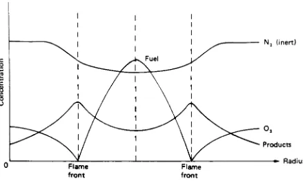
and product concentration.

The

concentration profiles

for

the oxidant,

fuel

and products across a

diffusion

flame

front

and

inside

the

flame

at a

constant

height

above

injection

ports

(above

any

recirculation

zone)

are shown

in Figure

N,

(inert)

[image:20.562.64.503.89.351.2]

The

flame

is

initially

characterized

by

how

the

fuel

and air are

physically

brought

together,

as either a

premixed

flame

or a

diffusion

flame. For

a premixed

flame,

the

airand

the

fuel

are

intimately

mixed

in

non-combustion

conditions,

then

ignited

and supplied with

additional air

to

insure

complete combustion.

For

a

diffusion

flame,

the

airand

the

fuel

are unmixed prior

to

ignition,

and mix

directly

at

the

flame front

itself (or

in

the

recirculation region aswill

be

seen

later in

the

Sections

5,

6

and

7).

The flame is further

characterized

by

the

flow

characteristics of

the

injected

fuel

mixture

(for premixed)

and/or

the

characteristics of

the

gas stream

in

which

the

fuel is

injected

(for

diffusion).

Flames

are also classified as

laminar

or

turbulent.

Laminar

flames

tend to

be

much steadier and

stable,

with awell

defined flame

length

and

shape;

while

turbulent

flames

are often

unsteady

and

wrinkled,

withan overall

oscillating

flame

length.

Turbulent

flames

do, however,

offer some

distinct

advantages over

laminar

flames. Their

burning

rate

is

much

higher

as

their turbulent

and wrinkled nature

greatly

increases

the

amount of surface area on

the

flame

front,

and

there

is

generally

more

intense fuel

oxidant

mixing

caused

by

the

turbulent

nature of

the

flame.

Both

of

these

characteristics

tend

to

increase

flame

efficiency,

but decrease flame

stability.

As

this

is

the

case,

in

practical

applications measures must

be

taken

to

stabilize

turbulent

flames before

these

benefits

can

be

realized.

3.13 Flame Stabilization:

The basic

principle

involved in flame

stabilization

is

quite simple.

Every

flame has

a

The flame

speed

is

a

measure

of

how quickly

the

flame

can consume

incoming

fuel

If

combustion

is

initiated

in

a

flowing

stream,

and

if

the

gas

velocity U

is

higher

than this

flame

speed

S,

the

flame

will move

downstream

at a speed of

U

minus

S. If

the

burning

velocity

is

higher,

than

the

flame

will move upstream witha speed of

S

minus

U.

Only

when

U

equals

S (or if U is less

than

S

and

there

is

anobstruction

to

block

the

flame from

traveling

upstream)

will

the

flame

be stationary

and stable.

In

order

to

achieve

the

required

stability for

a

flame in

conditions adverse

to

combustion,

such as

in

high velocity

gas

streams and

low

inlet

temperatures

(as in

aircraft

engines)

or

for

awiderangeof

operating

conditions

(as

in

gas

turbine engines),

one must use some

form

of

flame

holder.

The

function

of a

flame

holder is

to create,

in

a

high

speed gas

stream,

a region

whose

velocity

is

lower

than

the

burning

velocity

of

the

mixture

(the

recirculationzone).

Flame

blowout

occurs when

the

burning

velocity

of

the

flame is

below

the

gas speed at all

points

in

the

flow

field.

Thus

the

primary design

objective

for

good

stability is

to

maximize

the

ratio of

burning

velocity

to

flow

velocity;

incidentally

this

is

also a major requirement

for high

combustion efficiency.

The

most common

form

of

flame

stabilizer

is

the

bluff

body

flameholder.

Bluff

body

flameholders

operate

by

the

insertion

ofa non streamlined

body

into

the

gas

stream;

causing

arecirculationzone of

greatly decreased

gas

velocity

(TJ) immediately

after

the

body,

followed

by

a

turbulent

wakeregion

that

follows further downstream.

This,

in

effect,

increases flame

stability

by

effectively

lowering

U for

the

area of

the

gas stream

in

which

the

combustion will

take

place.

A

shearregion

is

created

between

this

recirculation

it into

the recirculation

zone

for

stable combustion.

Most

of

the

hot

combustion products

then travel

downstream

through the wake, though

someare pulled

back

into

the

shear

region and are passed

into

the

recirculation

zone

to

heat up

the

reactants.

Figure 3.2

gives

sample visualized

flow

around some standard

bluff

bodies,

by

Isaac,

Chidananda

and

Sridhara(1976).

As

this

form

of

flameholder is

usually

located in

a

duct,

hence

a

very important

characteristic

becomes

its

geometric

blockage

ratio

(BR)

as:

Duct

Free

Flow Area

Blockage

Area

and a relation

for

the

blockage

ratio

to the

aerodynamic

drag

is

as

follows:

(1_3A)2-1=

E(BRX1-BR)2

(3.6)

as

BA

is

the

aerodynamic

blockage,

and

E

is

a constant

based

on

the

flameholder

geometry.

For

concentric obstructed

jets:

BR=D^Dt

(37)

3.2

BluffBody

Flameholders:

There

has

been

a significant amount of research reported on

bluff

body

stabilized

flames

through

the years,

and

Lefebvre

(1983)

reports

that

extensive

data

and empirical

formulations

are available

in

order

to

predict

the

performance of a

bluff

body

stabilized

diffusion

flame.

Figure 3.2 Flow Pattern

around

various

Bluff Bodies

(a)

30

V-gutter,

BR

=

0.31

(b)

30

Round-nose,

BR

=

0.25

The

bluff

body

flameholder

has been

studied

in

both

cold

flow

and combustion

conditions,

as

both

yield

insights into its

_performance.

A

_cold

flow

_analysisofa

flameholder is

generally

an

examination

of

the

recirculation

and

mixing

characteristics of

the

systemunder

non-combustion

conditions.

A

combustion

analysis

is

performedunder combustion

conditions,

and

generally

focuses

on

flame

shape,

stability

and combustionefficiency.

It

is

seen

that the

focus

of most research

in

this

area

is

the

structure,

strength and size of

the

recirculation

zone,

and

its

effects on

flame

stability

and efficiency.

Li

and

Tankdn

(1987)

provide a goodoverview

of some of

the

research

done

in both

cold

flow

and

combustion,

aswellas provide

details

of

their

own visual studies.

A

significant amount ofresearch

has

been

reported

in

this

area,

and

recent work of

interest

to this

study

is

briefly

discussed below.

Nikjooy,

So

and

Peck

(1988)

offer

finite

rate

chemistry

models

(analytical)

to

predict

the

reaction region of swirl stabilized and single

bluff

body

obstructed non-premixed

flames,

as

wellas comparisons

to

their

experimental

data.

They

found

not

only

that their

finite

rate

chemistry

model wasadequate

to

predict

jet

stabilized

flames,

but

also

that

a

k-epsilon

turbulence

model proved

to

be

sufficient

for

non-premixed

flames

over a

fair

range of

operatioa

Pan,

Schmoll

and

Ballal

(1992),

conducteda

detailed

analysis of

the turbulence

properties and of

the

recirculation zonestructure ofa conical

bluff

body flameholder,

confined

withina can-type combustionchamber.

They

presented experimental

data encompassing

the

differences in

the

recirculationzone

between

openair and confined

flames.

Shefer,

Namazian

and

Kelly

(1989,

94)

presentsome of

the

effects of

bluff

body

stabilization

in

severalvisualization studies.

They

present results not unlike

those

of

Huang

and

Lin

(1994)

as will

be

seen

in

Section

3.3,

noting

the

significance of momentum

dominance

on

the

structure of

the

recirculation

zone.

There

are

significant amounts

of

ongoing

research

in

this

area,

but

most seems

to

be

aimed at

performance

analysis of specific engines and combustion

chambers,

rather

than

fundamental investigations

into

the principles

of

flame

stabilization.

3.3 Review

of

Single

BluffBody

Cold

Flow

Analysis

The

visual

study

of

Huang

and

Lin

(1994),

on

the

recirculation zoneof single

bluff

body

flameholder is

of particular

interest

to this

investigation,

and

is

usednot

only

to

validate

the

CFD

software,

but

also as a comparison

for

performance of

the

flameholder

Their

experimental

setup

consisted of a central air

jet

of

3.4

mm outer

diameter,

and an

annular

jet

of

30

mm outer

diameter,

obstructed

by

a

20

mm

diameter disc

of

0.44

blockage

ratio.

Using

a smoke wire

technique,

Huang

and

Lin

wereable

to

determine

the

shape and size of

the

recirculationzonecreated

by

two

concentric

jets

undervarious

inlet

conditions

(for

both

the

central and

the

annular

jet).

Four

typical

characteristic regions

were

identified

-that

ofweak

flow,

prepenetration,

transition,

and penetration.

Figure

3.3

illustrates

these

characteristic regions.

The

most

influential

factor

of

these

regions

is

the

dominance

in

axial momentum of one

jet

over

the

other, this

being

the

major

influence

on

stability.

The

weak

flow

region

(Region

I)

is

characterized

by

a

very

weakrecirculation

zone,

as

the

velocitiesof

the two

jets

are

too

low

to

createsignificant recirculation.

The

prepenetration region

(Region

II),

is

characterized

by

a

strong

recirculation

zone,

which

is

formed

as

the

momentum of

the

reverse axial

flow

from

the

annular

jet

overcomes

that

of

the

central

jet. This

region

is

further

categorized

into

three

sub-regions

(A),

(B)

and

(C),

with

the progression

leading

towards

a

less dominant

annular

jet,

and a recirculation zone

smaller

in

structure.

The

transition

region

(Region

III)

is

that

in

which

the

momentum of

the

central

jet begins

to

overpower

the

momentum of

the

annular

jet,

and

it

begins

to

pierce

through

and

break

up

the

recirculationzone.

It has

also

been

observed

that this

region

is generally

very

chaotic and

unstable,

often accompanied

by

violent and random

distortions in

the

shape of

the

recirculation zone.

The

penetration region

(Region

IV)

is

characterized

by

a split recirculation

zone,

where

the

momentum of

the

central

jet

overpowers

that

of

the

annular reverse axial

flow,

and

the

central

jet

column pierces

completely

through the

recirculation area.

This

causes a

division in

the

recirculation

zone,

resulting

in

a

ring

shaped

zone,

appearing

as

two

smaller sub zones

between

the

central

and annular

jets

when viewedacross

the

cross section.

Table

3.1

shows

the

results of

the

visualization

study,

most

notably

that the

height

of

the

recirculationzone

steadily

decreases

as

the

operating

conditions of

the

flameholder

move

towards the

penetration

region,

from

1.10

and

1

.20

DA

for

cases

n

(B)

and

II

(C)

down

to

0.70

for

case

IV

(B).

Table

3.1)

Sample Results

of

Huang

and

Lin,

Visualization

Study

uA

(m/s)

Uc

(m/s)

BR

(-)

Approx. Height

of

Rec. Zone

(DA)

Case

11(B)

0.75

1.79

0.44

1.10

H(C)

0.56

2.03

0.44

1.20

III

0.32

1.52

0.44

1.00

1.00

(m/s)

0.00

0

.5

2.0

2.5

3.0

3.5

Uc

(m/s)

4.0

COMPUTATIONAL FLUID

DYNAMICS

OVERVIEW:

4.1

Operation Principles

of

CFD:

A

commercial

CFD

code,

CFDS-Flow3D,

was used

to

perform

the

numerical analyses

in

the

present

investigation. CFDS-Flow3D is

a

finite

volume

CFD

code,

with

the

capabilities

of

solving

three-dimensional,

compressible and

turbulent

flows

of multiplegasand/or

liquid

constituents.

The

code solves

the

conservation equations of

mass,

momentumand

energy

(Navier Stokes

equations) in

discrete

cells,

based

upon user

defined

boundary

conditions,

to

obtain

the

steady

state solution

for

the

flowfield.

Specifically,

these

equationsare

the

continuity

equation

^

+

V(pU)

=

0,

(4.1)

dt

the

momentum equation

^+V(pUU)

=

B

+

V-a,

(4.2)

dt

sigma

being

the

stress

tensor

o=-p6+n(VU +

(VU)T),

(43)

and

the

energy

equation

^

+

V-(pUH)-V.(WT)

=

^,

(4.4)

dt

oi

The

code employs either a

k-epsilon

model or one of several variations of a

Reynolds

stress model

for

turbulence,

and

the

k-epsilon

model

is

used

exclusively

for

this

investigation.

The k-epsilon

model uses an

eddy viscosity hypothesis

for

the turbulence

ofthe

fluid flow.

This

model alters

the solution

of

the

Navier

Stokes

equations

by

replacing

the

fluid

viscosity

with an

effective

viscosity,

that

accounts

for

the turbulence

of

the

fluid

flow,

as

M-cfr

= _{u + pT.}

(4.5)

For

this

model

it is

assumed

that

HT=C,p-(4.6)

The

transport

equations

for

the

turbulence

kinetic

energy

(k)

and

the

energy dissipation

rate

(e)

are:

^pk

_,

uT

-r-+

V-(pUk)-V-((u

+

-^L)Vk)

=

P

+

G-pe

(4.7)

and

^

+

V-(pUe)-V-((u

+

-^)Ve)

=

dt

oe

e

e2

C,

-(P

+

C2

rnax(G,0))

-

C3p--(4.8)

A

mixed-is-bumt model

is

employed

for

gaseous combustion.

This

solution method

is

designed

for modeling diffusion

flames,

and approaches

the

solution

from

the

context

that

oxidant and

fuel

cannot

occupy

the

same space without reacting.

This

model solves

for

the

instantaneous

mixture content of each cell

in

terms

of

the

fuel,

oxidant and

product,

aswellas

the

variance

in

these

values

between iterations.

Each

cell

may

only

contain either

fuel

and

products or oxidant and products

(either

a rich or a

lean

mixture),

as all reactants

instantaneously

create products and release

the

heat

of combustion ofthe

fuel.

For

fast

rate

chemical

reactions,

the

mixture

fraction

(f)

can

be defined

as:

f

=

^lL_

(4 9)

l-(F/ASt01c)-'

(49)

where

m0

*=m{~T7AT~

(410)

and

the

stoichiometric

mixture

fraction

(Fyr)

is defined

as

F"

=

l

i+-i-

F/A

(4H)

r /a._Stoic

The

mixture

fraction is further

related

to

the

mass

fractions

of

fuel

(mf),

oxidant

(m,,)

and

products

(rrip) by

the

following

f-F

mf

=

i_

'

m

=

'

and

mp

=

l

~

mf

(4-12)

for fuel rich

cells,

and

f

mf =0,mo

=

l--,andmp

=

l-m0

(4

13)

*Vr

The

mixture

fractions

and

their

variances

(which

are calculatedwithan extensive

probability

function)

are calculated

along

with

the

conservation

laws

until convergence criteria

(the

minimization of residuals

for

all

variables)

are obtained

for

the

steady

state solution.

A

separate computational model

is

used

for

each of

the

numerical analyses

presented,

one

for

the

single

bluff

body

analysis

(for

both

the

validationand

the

propane

analyses),

one

for

the

double

bluff

body

cold

flow

analysis,

and one

for

the

double bluff

body

combustion

analysis.

The

single

bluff

body

model

is based

on

the

geometry

of

the

experimental

setup

of

Huang

and

Lin,

and

the

double bluff

body

model

is based

on

the

geometry

of

the

experimental

setup

as presented

in Section

7.0. Each

modelconsists of a

three-dimensional

solution

field

that

encompasses

the

desired

region of

the

flow

field,

internal

solidcells

to

model

the

nozzle

geometry,

and

boundary

conditions

to

_model

the

flow

_conditions.

The

_solution

field is

divided

into discrete

cells

(control

volumes) for

computationalsolution.

As only

a

two-dimensional

axisymmetric

model

in

the

axial and radial

directions is

needed

for

each

analysis,

the

solution

field is

a single cell

in height

and a

two-dimensional

solutionmethod

is

employed

by

the

solver

The

boundary

conditions employed

for

the

air and

fuel inlets

of

the

nozzlewere

turbulent

uniform

velocity

boundaries,

placed at

the

base

of

the

nozzle.

Ambient

pressure

boundaries

wereemployed

along

the

sidesof

the

model

to

simulate anopenair

diffusion

flame

A

mass

flow

outlet at

the

top

of

the

model allows all mass

entering

the

system

(solution

field)

to

leave,

in

accordancewith

the

law

of conservationof mass.

4.2

Numerical Model

for Single

BluffBody:

The

computational

model

for

the

single

bluff

body

validationanalysis

(Section

5.0),

consists

of a

solution

field

of

6

cm

by

10

cm,

divided into

6000

cells,

60

cells

equally

spaced

horizontally

in

100

vertical rows.

The

model

encompasses

a

full

cross-section of

the

flameholder,

and

the

solution method

recognizes

the

model as an axisymmetricsection.

Figure

4.

1

shows

the

outline of

the

model

geometry,

figure

4.2

shows

the

placement of

the

boundary

conditions,

and

figure

4.3

shows

the

structure of

the

grid

(cells). The

nozzle

geometry

was

modeled as solid

cells,

withno

slip

boundary

walls,

and

has

a

30

mm exit

diameter for

the

annular

jet,

obstructed

by

20

mm

disc

(DA)

as

in

the

experimental

setup

of

Huang

and

Lin.

The

exit

diameter

of

the

central

jet

was

increased

to

4

mm

(from 3.4

mm)

in

order

to

serve

as a

better

comparison

for later

sections,

as

it

allowed

for

a grid structure more similar

to

later

models.

The

magnitude of

the

central

jet

velocity

(Uc)

has

been

modified

for

allcases

(and

retermed

the

modified central

jet

velocity

(Umc)),

to

maintain

the

samevolume

flowrate

as

those

studied

experimentally

by decreasing

the

axial

velocity in

accordance

with

the

increase

in

area.

The

nozzle section accounts

for

the

lower 3

cm of

the model,

leaving

7

cm of solution

field

in

the

wake region.

The

velocities of

the

central

(Umc)

and

annular

jets

(Ua)

are

given

in Table

4.1.

The only

appreciable

difference between

the

cold

flow

validation modeland

the

cold

flow

model withpropane

is

that

a second

fluid is

present,

so

the

solution method must account

for fluid

mixing.

Table

4.1)

Single

BluffBody

Analysis

Case

uA

Uc

uMC

BR

k

6

11(A)

0.75

1.4

1.0

0.44

0.00196

0.10026

n<B)

0.75

1.79

1.28

0.44

0.00329

0.18499

H(C)

0.56

2.03

1.45

0.44

0.00423

0.26983

ni

0.32

1.52

1.09

0.44

0.00237

0.11327

IV

(B)

0.47

2.96

2.12

0.44

0.00899

0.83651

Table

4.2)

Double

BluffBody

Cold

Flow Analysis

Case

<D

BR

uA

Uc

k

e

Alpha

1.0

0.53

2.732

2.282

0.01491

0.21702

Beta

1.5

0.53

2.732

3.423

0.01491

0.21702

Chi

1.0

0.44

2.732

2.282

0.01491

0.21702

Mass Row

Boundary

a c 3

O CO

CO

c u

S

<

Walls

>

i. i- _i.

A

"O c 3

o CQ

2

3

03

1

c

E

<

A

A

n

A

-- a

Air

Air

(Fuel)

Air

Velocity

Inlets

'I

a

a aaaaaaaaaaaaa !

iiiitiiiiiitiiiiiiiiiiiiiii

i I

^>

1 1 1 1 1 1 m 1 1

1 t+i

=ffl

iiiini

-;!>

I i

mini mmmmiiiiiiiiii

""!!!!!!!!!!!!!!!!!

;::::::::::>

"""":::"":"!:

a

iaiitsiiaaaaaaaaBiaaaaaaaaiaiaBaaaaaBafaaBiaaaBaaaaaaaa

a*ala>,a*1""""1"

iiaii iiiiiiiiii an ""

i aiiiiii

!!!!"!"!

' Ill

SBaa.BaaaaBiBaBBiBaaaBBaBiaaaBaBjBaaBaaaBjBajBaBBBBaBa

'*l^"*',,'*i"'*""1112IJ

4.3 Numerical

Model

for

Double

BluffBody

-

Cold Flow:

The

computational

model

for

the

cold

flow

double bluff

body

analysis

(Section

6.1)

is

3

cm wide

by

10

cm

tall,

and consists of

12000

cells,

60

cells

equally

spaced

horizontally

in 200

vertical rows.

Figure

4.4

shows

the

outline

of

the

model

geometry

(note

that

D0

is dependent

on

the

geometric

blockage

ratio of

the

disc,

and

is

28.0

mm

for

BR

=

0.53

and

is

26.0

mm

for

BR

=

0.44),

figure

4.5

shows

the

placement of

the

boundary

conditions,

and

figure

4

6

shows

the

grid structure.

The

blockage

ratio

for

the

central

jet

obstruction

is

0.57.

There

are

two

significant

differences between

this

model and

that

of

the

single

bluff

body

flameholder.

First,

the

grid

density

was

increased

to

account

for

the

finer

geometry

of

the

central

bluff

body;

and

second,

the

model

only

encompasses an axisymmetric section

from

the

centerline

outward,

essentially

half

the

size of

the

previous model.

A symmetry

plane

has

been

added at

the

centerline of

the

flameholder

in

order

to

model

the

effectsof

the

entire cross-section.

The

nozzle

geometry

was modeled

in

the

same manner as

the

previous models

(as

solid

cells),

and

again encompasses

the

lower

3

cm of

the

model,

leaving

7

cm ofsolution

field

for

the

wake

region.

The

central

(Uc)

velocity

is for

propane and annular

(UA)

velocity

is for

air,

and

two

separate geometric

blockage

ratios

(for

the

air

obstruction)

were

examined,

allare as given

in

Table 4.2.

Otherwise

the

solution method

is

identical

to

that

of

the

single

bluff

body

propane

extensionmodel.

85.0

mm

15.0

mm

< >

5.0

mm

-

4.0

_mm

*

18.0

mm

30.0

mm

2.0

mm

Mass Flow

Boundary

o

c 3

O

CD

3

co

CO

!

_C

<U

E

<

A

Walls

A

ji i. i.

CL

E

E

Air

Fuel

Velocity

Inlets

4.4 Numerical

Model for

Double

BluffBody

-

Combustion:

The

computational

model

for

the

double

bluff

body

combustionanalysis

(Section

6.2)

consists of

three

solution

fields

(termed

blocks

in

the

CFDS-Flow3D

command

code),

joined

together.

The

first

contains

the

internal

solids and

flow

passages

for

the nozzle,

while

the

other

two

are

for

the

downstream

region.

As

the

first

section

is

of

significantly less

width

than the

third,

the

second section

is

tapered to

allow

for

smooth

transition

between

them.

The

first

section

is

5

cm wide

by

1

.5 cm

tall, containing

3000

cells,

100 equally

spaced

horizontally by

30 equally

spaced

vertically

(note

that

eachsection/blockcontains

the

samenumber of

horizontal

cells

for

continuity).

The

second section

is

3

cm wide at

the

base,

20

cmwideat

the

top,

13.5

cm

tall,

and contains

4000

cells.

The

third

section

is

20

cmwide

by

25

cm

tall

and

contains

4000

cells,

divided into

40

rows

in

averticalgeometrical progression.

The

geometric

progression

increases

the

height

of each cell

in

accordance with

its distance

form

the

base,

so

the

grid

is

essentially

finer

at

the

base

of

the

block,

and courserat

the

top

of

the

block. Figure

4.7

shows

the

outline of

the

model

geometry,

figure

4.8

shows

the

placement of

the

boundary

conditions,

figure

4.9

shows

the

grid structure of

the model,

and

figure

4. 10

is

an enhanced

viewof

the

grid structure

in

the

first

block.. This

model

is

significantly larger

than

each of

the

previous models

(geometrically

speaking),

and again encompasses

the

axisymmetric section

from

the

centerline

outward,

witha

symmetry

plane at

the

centerline.

The

nozzle

geometry

is

defined in

much

the

same manner as

the

previoussections.

Again,

the

central

velocity

(Uc)

is

propane,

and

the

annular

velocity

(UA)

is

air,

and

two

geometric

blockage

ratios are

studied,

all

are as given

in

Table 4.2.

250.0

mm

Mass

Row

Boundary

a c 3 o

CQ

2

3

c

IS

E

Ambient

Pressure

Boundary

Nozzle

Boundary

Conditions

as

in

Figure 4.5

,:.-.v.-\^.^C*.\^vc^^^

aTaW '.--.'

\\\\^_XCS>X'X-Y>\<V\VX\\.V\\\V\\\CA\\\\\\\V0AV\V.\\\VHt>UV.HUH11\Hllll ">\ '^\-XV\C.W.".

"

\\\WVVW-_NC-V>\\VWWWAV.'.rtl'UhW U\ \\m.U\HU! Ii<1 1

. v.

'a',X\V'.\\v;.'

v.'.\s -v\-'\\\VVC.WV.V.'.VAXV^Mt'M.M'itt.'.U'.tlHir.ll

--\\vkV^-k-WV.Vk'-kVV.'VWWV.r.'-.W V.\ V-.'VA VO0Hv.\-IHHVVUMUUilll

Figure

4.10

Grid Structure for Double

BluffBody

4.5

Output

from

the

CFD Code:

CFDS-Flow3D

offers solution output

in

two

forms,

tabular

data

output

in

the

form

ofa

data file (as

seen

in

Appendix

X),

or graphical

output,

in

the

form

ofvector and

contour plots of

the

data.

For

the

purposes of comparison

the

latter

is

most

appropriate,

and

the

majority

of

the

computational results given

in

this

study

will

be

presented as

vectorand contour plots.

These

plots are available

for

eachvariable

that

is

solved

for in

the

code.

For

the

cold

flow

models of

the

single

bluff

body

and

the

double bluff

body

flameholders,

the

variables solved

for

included:

u

velocity,

v

velocity, pressure,

density,

viscosity,

k,

e,

enthalpy

and a single mass

fraction

(percent

of

fuel in

cell

by

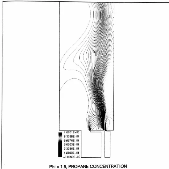
mass).

For

the

double bluff

body

combustion

models,

the

variables

included

all of

the

above,

aswell as:

temperature,

three

mass

fractions (one

for

percent

oxidant,

one

for

percent

fuel,

one

for

percent

products),

and

two

combustionscalars

(mixture fractions).

5.0

NUMERICAL

VALIDATION ANALYSIS:

5. 1

Cold

Flow

Analysis

of

Single BluffBody:

In

order

to

verify

the

capabilities

of

the

Computational

Fluid Dynamics Solver

Code,

part of

the

experimental research of

Huang

and

Lin

was recreated

numerically

with

the

code.

This

was undertaken

to

verify

the

capability

of

the

code

to

accurately

model

the

recirculation

zone,

and

later

to

serve as a

basis

of comparison

for

the

double bluff

body

configuration

The

initial

object of

this

validation was

to

clearly

reproduce

the three

characteristic

flow

regions

found

by Huang

and

Lin,

andshow

the

effects ofmomentum

dominance

on

the

recirculation zone.

Five

individual

cases were

studied,

based

on

those

of

Huang

and

Lin,

and are as

defined

in Table 4. 1. Of

all

the

output available

from

the

code,

the

axial

(V)

velocity

contours provide

the

clearest

depiction

of

the

structure of

the

recirculation

zone,

while

velocity

vectorplotsof

the

region show

the

effect of

the

recirculation zone.

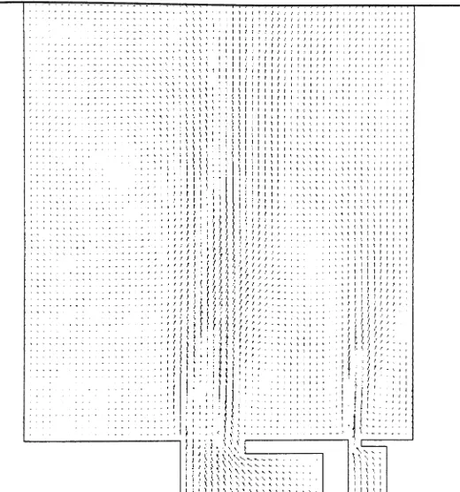
Figures 5. 1

through

5.10

depict

the

velocity

vectors and

V velocity

contours of

the

five

cases studied.

Cases

n

(A),

(B),

and

(C)

are representative of

the three

sub-regions of

the

prepenetrationregion.

Figures

5.1,

5.3, 5.5,

5.7

and

5.9

(the

velocity

vector

plots) clearly

show recirculation

behind

the

bluff

body

obstruction,

but

the

V velocity

contour plots

yield much

better

information

as

to the

structure of

the

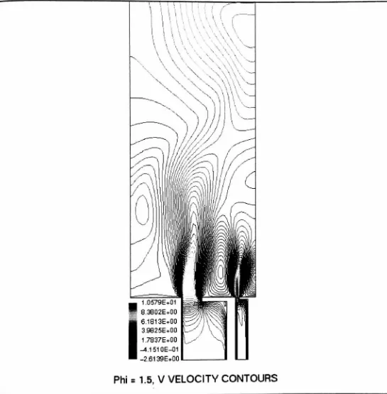
recirculation zone.

For

Case

II

(A),

Figure 5.2 clearly

showsa stablerecirculationzone

dominated

by

the

reverse

flow

of

the

annular

jet. This

is

evident

by

the

purpleregions which

denote

negative axial

velocity

(or

recirculation).

The

zone

has

the

expected closed

toroidal

shape similar

to that

shown

3.-3-&9ftB-!qi

Q.'^&oq^qq;

i

r

i i r i i

r

i

i

r

i . .

t 1 i I I i I , i I , i I

?

I I .

I

I

f

i i

r

i i

r

i i i i i i i i i i i i i i 1 i

4

4

i

*

r

r

f

I

f

r

MM,

i i

t

1

i 1

1 _j ,

,. i r 1 f < r t I I I I I I

\ \ \ \ i.

r 'i w

\

\ \

i i \

,

',

i

r i

f i

r . 1 s 1 . . .

r

m

i

r 1 1 i

\

1 1

? 1 i

,

i

i

i r . i 1 i i 1

1

.

1

1

1 i i

I

M 1

I

I

I I i r i r

I

t

r

r

i i i r 1 1 i r r

i i r t I I f I I } I

I

f

I

MM

r

1

f

t

1

I

.

1

.

1

r r 1

r r 1

r r 1

1 1 t . i r i i r . I f

1 i r .

1

r

1 i i i

l

i

1 i i

. 1 i

. 1 i

. i i t

I

i i i

1

t ,

1

l

i

1

l

i '

1

)

\

i

'i

I

i

'i

\

i i

'i i

i 'i i

i i i i i i i i i

(,

\

\

\

\

i

<

V \ 1 ,

\ \

s \ )

\

t \ 1

. * 1

t 1

< i i

. i i

i i 1 i i 1

, i i

Ji

\

i '.

\

i

'i

',

i

'i

1

i

i

.

, i i

i i i

t . i '.

5

' i

ri

\

r . i

i

' \ i

i *

I i 1 h

*

%

1

^

i

, , k 1

i

1 1 ' i i t 1

'

[

I 1. *

.

ii

f s / /

,

/ f

1

1

1 1

I

t

f

I ?

I

I

t

M M

r ) f

) t f

r t t

f

t

I , 7

i1

r