A SAM Based Global CGE Model using GTAP Data January 2005

This is a repository copy of A SAM Based Global CGE Model using GTAP Data January 2005 .

White Rose Research Online URL for this paper: http://eprints.whiterose.ac.uk/9907/

Monograph:

McDonald, S., Robinson, S. and Thierfelder, K. (2005) A SAM Based Global CGE Model using GTAP Data January 2005. Working Paper. Department of Economics, University of Sheffield ISSN 1749-8368

Sheffield Economic Research Paper Series 2005001

[email protected] https://eprints.whiterose.ac.uk/

Reuse

Unless indicated otherwise, fulltext items are protected by copyright with all rights reserved. The copyright exception in section 29 of the Copyright, Designs and Patents Act 1988 allows the making of a single copy solely for the purpose of non-commercial research or private study within the limits of fair dealing. The publisher or other rights-holder may allow further reproduction and re-use of this version - refer to the White Rose Research Online record for this item. Where records identify the publisher as the copyright holder, users can verify any specific terms of use on the publisher’s website.

Takedown

If you consider content in White Rose Research Online to be in breach of UK law, please notify us by

Sheffield Economic Research Paper Series

SERP Number: 2005001

Scott McDonald*, Sherman Robinson and Karen Thierfelder

A SAM Based Global CGE Model using GTAP Data

January 2005

* Corresponding author

Department of Economics University of Sheffield 9 Mappin Street Sheffield

S1 4DT

United Kingdom

Abstract

This paper provides a technical description of a global computable general equilibrium (CGE) model that is calibrated from a Social Accounting Matrix (SAM) representation of the Global Trade Analysis Project (GTAP) database. A distinctive feature of the model is the treatment of nominal and real exchange rates and hence the specification of multiple numéraire.

Keywords: Computable General Equilibrium; GTAP.

JEL numbers: D58; R13; F49.

1. INTRODUCTION

This paper provides a technical description of a variant of a Social Accounting Matrix (SAM) based Global Computable General Equilibrium (CGE) model that has been calibrated using data derived from the Global Trade Analysis Project’s (GTAP) database. The model is a member of a family of CGE models that model trade relationships using principles described in the 1-2-3 model (de Melo and Robinson, 1989; Devarajan, et al., 1990). More specifically this model is a direct descendant of an early US Department of Agriculture model (see Robinson et al., 1990) and a model that was developed to evaluate the NAFTA (Robinson et

al., 1993). However numerous features of this model stem from other developments in CGE

modelling over the last 10 years; some of these sources of inspiration are direct and easily identified, e.g., the IFPRI standard model (Lofgren et al., 2002) and the PROVIDE Project model (McDonald, 2003), others are indirect and easily identified, e.g., the GTAP model (Hertel, 1997), while others are both direct and indirect but less easily identified. In addition the model owes a lot to the development of the SAM approach to national accounting, e.g., Stone (1962a and b) and Pyatt (1991), and the SAM approach to modelling, e.g., Pyatt (1987), Drud et al., (1986).

The underlying approach to multi-region modelling for this CGE model is the construction of a series of single country CGE models that are linked through their trading relationships. As is common with all known CGE models the price system(s) in the model are linear homogenous and hence the focus is upon movements in relative, rather than absolute, prices. Consequently each region in the model has its own numéraire price, typically the consumer price index (CPI), and a nominal exchange rate, while the model as a whole requires a numéraire, typically the exchange rate of a reference region. As such this model contains a fundamentally different philosophical approach to global modelling to that found in the GTAP model.1 Behind this difference lies a deep theoretical debate about how

comparative static and finite horizon dynamic CGE models should value transfers associated with the capital account of the balance of payments (see Robinson, 2004).

The rest of this paper is organised as follows. Section 2 reviews the data used in the model; this section also provides a brief description of how the data were transformed from the GTAP database into a SAM. This is followed in section 3 by a descriptive overview of the

model and then, in section 4, by a formal description of the model’s equations. The

description in section 4 is based upon a default setting for the model closure rules; one of the model’s key features is the flexibility of the closure rules and consequently section 5

considers the alternatives built into the model’s basic structure. All global CGE models are large and therefore present a series of potential implementation problems; section 6 briefly reviews some of the programmes that have been developed to support the basic model and provides some guidelines for use of this class of model. The paper ends with some concluding comments that primarily focus upon planned model developments.

2. MODEL DATA

The data used in the model were derived from the GTAP database (see Hertel, 1997) using a three dimensional Social Accounting Matrix (SAM) method for organising the data. Details of the method used to generate a SAM representation are reported in McDonald and

Thierfelder (2004a) while a variety of reduced form representations of the SAM and methods for augmenting the GTAP database are reported in McDonald and Thierfelder (2004b) and McDonald and Sonmez (2004) respectively.2 Detailed descriptions of the data are provided elsewhere so the discussion here is limited to the general principles.

GLOBAL SOCIAL ACCOUNTING MATRIX

The Global SAM can be conceived of as a series of single region SAMs that are linked through the commodity trade accounts; this is particularly valid in the context of the GTAP database since the ONLY way in which the regions are linked directly in the database is through commodity trade transactions although there are some indirect links through the demand and supply of trade and transport services. Specifically the value of exports valued free on board (fob) from source x to destination y must be exactly equal to the value of

imports valued fob to destination y from source x, and since this holds for all commodity trade transactions the sum of the differences in the values of imports and exports by each region must equal zero. However the resultant trade balances do not fully accord with national accounting conventions because other inter regional transactions are not recorded in the database (see McDonald and Sonmez, 2004). A description of the transactions recorded in a representative SAM for a typical region in the database is provided in Table 1.

2

A SAM is a transactions matrix; hence each cell in a SAM simply records the values of the transactions between the two agents identified by the row and column accounts. The selling agents are identified by the rows, i.e., the row entries record the incomes received by the identified agent, while the purchasing agents are identified by the columns, i.e., the column entries record the expenditures made by agents. As such a SAM is a relatively

Table 1 Social Accounting Matrix for a Region in the Global Social Accounting Matrix

Commodities Activities Factors Households Government Capital Margins Rest of World Totals

Commodities 0

Combined

Intermediate Use

Matrix

0 Private

Consumption

Government

Consumption

Investment

Consumption

Exports of Margins

(fob)

Exports of

Commodities (fob)

Total Demand for

Commodities

Activities Domestic Supply

Matrix 0 0 0 0 0 0 0

Total Domestic

Supply by Activity

Factors 0 Expenditure on

Primary Inputs 0 0 0 0 0 0

Total Factor

Income

Households 0 0 Distribution of

Factor Incomes 0 0 0 0 0

Total Household

Income

Government Taxes on

Commodities Taxes on Production Direct/Income Taxes Direct/Income

Taxes 0 0 0 0

Total Government

Income

Capital 0 0 Depreciation

Allowances Household Savings

Government

Savings 0

Balance on

Margins Trade Foreign Savings Total Savings

Margins

Imports of Trade

and Transport

Margins

0 0 0 0 0 0 0 Total Income from

Margin Imports

Rest of World Imports of

Commodities (fob) 0 0 0 0 0 0 0

Total Income from

Imports

Totals Total Supply of

Commodities

Total Expenditure

on Inputs by

Activities Total Factor Expenditure Total Household Expenditure Total Government

Expenditure Total Investment

Total Expenditure

on Margin Exports

Total Expenditure

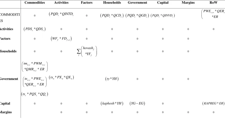
Given these definitions of a SAM the transactions recorded in a SAM are easily interpreted. In Table 1 the row entries for the commodity accounts are the values of commodity sales to the agents identified in the columns, i.e., intermediate inputs are purchased by activities (industries etc.,), final consumption is provided by households, the government and investment demand and export demand is provided by the all the other regions in the global SAM and the export of margin services. The commodity column entries deal with the supply side, i.e., they identify the accounts from which commodities are

purchased so to satisfy demand. Specifically commodities can be purchased from either domestic activities – the domestic supply matrix valued inclusive of domestic trade and transport margins – or they can be imported – valued exclusive of international trade and transport margins. In addition to payments to the producing agents – domestic or foreign – the commodity accounts need to make expenditures with respect to the trade and transport

services needed to import the commodities and any commodity specific taxes.

The GTAP database provides complete coverage of bi lateral transactions in

An important feature of the construction of a SAM can be deduced from the nature of the entries in the commodity account columns. By definition the columns and row totals must equate and these transaction totals can be expressed as an implicit price times a quantity and the quantity of a commodity supplied must be identical to the quantity of a commodity demanded. The column entries represent the expenditures incurred in order to supply a commodity to the economy and hence the implicit price must be exactly equal to the average cost incurred to supply a commodity. Moreover since the row and column totals equate and the quantity represented by each corresponding entry must be same for the row and column total the implicit price for the row total must be identical to average cost incurred to supply the commodity. Hence the column entries identify the components that enter into the

formation of the implicit prices in the rows, and therefore identify the price formation process for each price in the system. Typically a SAM is defined such that the commodities in the rows are homogenous and that all agents purchase a commodity at the same price.

Total income to the activity accounts is identified by the row entries. In the simple representation of production in the GTAP database each activity makes a single commodity and each commodity is made by a single activity, which means that the domestic supply matrix is a square diagonal matrix. The expenditures on inputs used in production are recorded in the activity columns. Activities use intermediate inputs, which in this version of the database are record as composites of domestically produced and imported commodities, primary inputs and pay taxes on production. For each region the sum of the payments to primary inputs and on production taxes by activity is equal to the activity’s contribution to the value added definition of GDP while the sum over activities equals the region’s value added measure of GDP.

stems from the reduced form representation of intra institutional transactions provided by the GTAP database (see McDonald and Thierfelder, 2004b).3 There are therefore five sources of savings in each region: depreciation, household/private savings, government savings, balances on trade in margin services and balances on trade in commodities, but only a single

expenditure activity – investment (commodity) demand.

As should be apparent from the description of the SAM for a representative region the database is strong on inter regional transactions but relatively parsimonious on intra regional transactions.

DATABASE DIMENSIONS

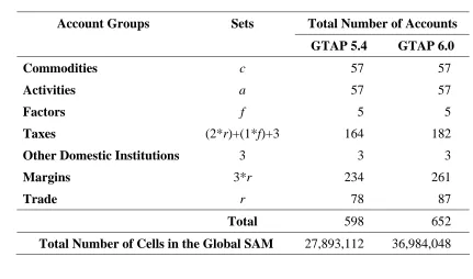
The dimensions of the SAM are determined by the numbers of accounts within each

aggregate group identified in Table 1, while the actual numbers of accounts in each group of accounts are defined for version 5.4 and 6.0 of the GTAP database in Table 2. Given the large number of accounts in the SAMs for each region and the relatively large number of regions the total number of cells in the global SAM is very large, although only slightly over 10 percent of the cells actually contain non zero entries; nevertheless this still means that the GTAP database contains some 4 million transaction values, which implies that there are some 8 million possible prices and quantities that can be deduced from the database. Even allowing for the implications of adopting the law of one price for transactions in the row of a each region’s SAM and for other ways of reducing the numbers of independent prices and

quantities that need to be estimated in a modelling environment,` it is clear that the use of the GTAP database without aggregation is likely to generate extremely large models (in terms of the number of equations/variables). Consequently, except in exceptional circumstances all CGE models that use the GTAP data operate with aggregations of the database.

3

Table 2 Dimensions of the Global Social Accounting Matrix

Account Groups Sets Total Number of Accounts

GTAP 5.4 GTAP 6.0

Commodities c 57 57

Activities a

f

titutions 3 3 3

23 261

Total 598 652

57 57

Factors f 5 5

Taxes (2*r)+(1* )+3 164 182

Other Domestic Ins

Margins 3*r 4

Trade r 78 87

Total Number of Cells in the Global SAM 27,893,112 36,984,048

3 OVERVIEW OF THE MODEL

BEHAVIOURAL RELATIONSHIPS

The within regional behavioural relationships are simple in this variant of the model; it is easy

een te

rtion

The Armington assumption is used for trade. Domestic output is distributed between the dome

nd

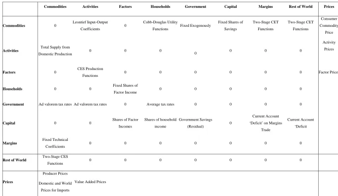
to make them more complex but the focus in this variant of the model is upon international trade relationships. The activities are assumed to maximise profits using technology characterised by Constant Elasticity of Substitution (CES) production functions betw primary inputs and Leontief technology between aggregate primary inputs and intermedia inputs. The household maximises utility subject to preferences represented by a Cobb-Douglas utility function, having first paid income taxes and having saved a fixed propo of after tax income.4

stic market and exports according to a two-stage Constant Elasticity of Transformation (CET) function. In the first stage a domestic producer allocates output to the domestic or export market according to the relative prices for the commodity on the domestic market a the composite export commodity, where the composite export commodity is a CET aggregate

4

tion.

ditions

All commodity and activity taxes are expressed as simple ad valorem tax rates, while incom

of the exports to different regions – the distribution of the exports between regions being determined by the relative export prices to those regions. Consequently domestic producers are responsive to prices in the different markets – the domestic market and all other regions in the model – and adjust their volumes of sales according relative prices. Domestic demand is satisfied by composite commodities that are formed from domestic production sold

domestically and composite imports. This process is modeled by a two-stage CES func At the bottom stage a composite import commodity is a CES aggregate of imports from different regions with the quantities imported from different regions being responsive to relative prices. The top stage defines a composite consumption commodity as a CES aggregate of a domestic commodity and a composite import commodity with the mix being determined by the relative prices. Hence the optimal ratios of imports to domestic

commodities and exports to domestic commodities are determined by first order con

based on relative prices. The price and quantity systems are described in greater detail below.

Table 2 Behavioural Relationships for a Global CGE Model

Commodities Activities Factors Households Government Capital Margins Rest of World Prices

Commodities 0 Leontief Input-Output

Coefficients 0

Cobb-Douglas Utility

Functions Fixed Exogenously

Fixed Shares of Savings

Two-Stage CET Functions

Two-Stage CET Functions

Consumer Commodity

Price

Activities Total Supply from

Domestic Production 0 0 0 0 0 0 0

Activity Prices

Factors 0 CES Production

Functions 0 0 0 0 0 0 Factor Prices

Households 0 0 Fixed Shares of

Factor Income 0 0 0 0 0

Government Ad valorem tax rates Ad valorem tax rates 0 Average tax rates 0 0 0 0

Capital 0 0 Shares of Factor

Incomes

Shares of household income

Government Savings

(Residual) 0

Current Account ‘Deficit’ on Margins

Trade

Current Account ‘Deficit

Margins Fixed Technical

Coefficients 0 0 0 0 0 0 0

Rest of World Two-Stage CES

Functions 0 0 0 0 0 0 0

Prices

Producer Prices Domestic and World

Prices for Imports

Table 3 Transactions Relationships for a for a Global CGE Model

Commodities Activities Factors Households Government Capital Margins RoW

COMMODITI ES

0

(

(

)

c c

PQD QCD

(

)

(

)

, * ,

*

c w c w

PWE QER

ER

⎛ ⎜ ⎝

Activities

(

)

Factors 0

(

)

Households 0 0

* f

f f

hovash

YF

⎛ ⎞

⎜ ⎟

⎜ ⎟

⎝ ⎠

∑

Government

, ,

,

*

* *

w c w c

w c

tm PWM

QMR ER

⎛ ⎞

⎜ ⎟

⎝ ⎠

, ,

,

*

* *

w c w c

w c te PWE

QER ER

⎛ ⎞

⎜ ⎟

⎝ ⎠

(

)

(

)

(

)

Capital 0 0 0

(

)

(

)

(

)

Rest of World ,

,

* *

w c

w c PWMFOB

QMR ER

⎛ ⎞

⎜ ⎟

⎝ ⎠ 0 0 0 0 0 0 0

Government expenditure consists of commodity (final) demand, which is assumed to be fixed in real terms. Hence government saving, or the internal balance, is defined as a residual. However, the closure rules for the government account allow for various permutations. In the base case it is assumed that the tax rates and volume of government demand are fixed and government savings are calculated as a residual. However, the tax rates can all be scaled using the tax specific scaling factors; hence for instance the value of government savings can be fixed and one of the tax scalars can be made variable thereby producing an estimate of the constrained optimal tax rate. If the analyst wishes to change the relative tax rates across commodities (for import duties, export taxes and sales taxes) or across activities (for

production taxes) then the respective tax rate parameters can be altered via a second adjuster. Equally the volume of government consumption can be changed by adjusting the closure rule with respect the scaling adjuster attached to the volumes of government consumption. The pattern of government expenditure is altered by changing the parameter that controls the pattern of government expenditure (comgovconst).

PRICE AND QUANTITY SYSTEMS FOR A REPRESENTATIVE REGION

Price System

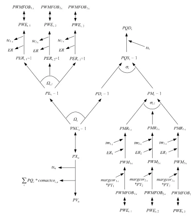
The price system is built up using the principle that the components of the ‘price definitions’ for each region are the entries in the columns of the SAM. Hence there are a series of explicit accounting identities that define the relationships between the prices and thereby determine the processes used to calibrate the tax rates for the base solution. However, the model is set up using a series of linear homogeneous relationships and hence is only defined in terms of relative prices. Consequently as part of the calibration process it is necessary set some of the prices equal to one (or any other number that suits the modeler) – this model adopts the convention that prices are normalised at the level of the CES and CET aggregator functions for PXC and PQS. The price system for a typical region in a 3 region global model is illustrated by Figure 1 – note that this representation abstracts from the Globe region.

The relationships between the various prices in the model are illustrated in Figure 1. The domestic consumer prices (PQD) are determined by the domestic prices of the

domestically supplied commodities (PD) and the domestic prices of the composite imports (PM), and by the sales taxes (ts) that are levied on all domestic demand. The prices of the composite imports are determined as aggregates of the domestic prices paid for imports from all those regions that supply imports to this economy (PMR) under the maintained assumption that imports are differentiated by their source region. These region specific import prices are expressed in terms of the domestic currency units after paying for trade and transport services and any import duties. Thus a destination region is assumed to purchase a commodity in a source economy where the price is defined in the source economies currency units and is valued free on board (fob), i.e., PWMFOB. The carriage insurance and freight (cif) price (PWM) is then defined as the fob price plus trade and transport margin services (margcor) times the unit price of margin services (PT). The cif prices are related to the domestic price of imports by the addition of any import duties (tm) and then converted into domestic currency units using the nominal exchange rate (ER).

exchange (PWE). Notice how the export prices by region of destination (PER) are all normalised on 1, but the seeming counterpart of normalising import prices by source region (PMR) are not normalised on 1. The link between the regions is therefore embedded in the identification of the quantities exchanged rather than the normalised prices and is a natural consequence of the normalisation process.

Figure 1 Price System for a Typical Region

,

*

c c a

c

PQ comactco

∑

Finally the value added prices (PV) are determined by the activity prices (PX), the production tax rates (tx), the input-output coefficients (comactco) and the commodity prices (PQD). The activity prices are a one to one mapping of the commodity prices received by activities (PXC); this is a consequence of the supply matrix being a square diagonal matrix.

Quantity System

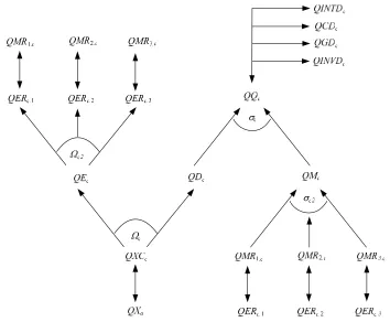
The quantity system for a representative region is somewhat simpler. The composite consumption commodity (QQ) is a mix of the domestically produced commodity (QD) and the composite import commodity (QM), where the domestic and imported commodities are imperfect substitutes. The composite import commodity is also an aggregate of the

commodity imported from different regions (QMR), which the equilibrium conditions requires are identical to the quantities exported by other regions to the representative region (QER). The composite consumption commodity is then allocated between domestic

intermediate demands (QINTD), private consumption demand (QCD), government demand (QGD) and investment demand (QINVD).

Figure 2 Quantity System for a Typical Region

a composite export commodity (QE) under the maintained assumption of imperfect transformation, and similar the composite export commodity is allocated between the different destination regions (QER) under the maintain assumption of imperfect transformation.

THE GLOBE REGION

An important feature of the model is the use of the concept of a region known as Globe. While the GTAP database contains complete bilateral information relating to the trade in commodities, i.e., in all cases transactions are identified according to their region of origin and their region of destination, this is not the case for trade in margins services associated with the transportation of commodities. Rather the GTAP databases identifies the demand, in value terms, for margin services associated with imports by all regions from all other regions but does not identify the region that supplies the margin services associated with any specific transaction. Consequently the data for the demand side for margin services is relatively

detailed but the supply side is not. Indeed the only supply side information is the total value of exports of margin services by each region. The Globe construct allows the model to get around this shortage of information, while simultaneously providing a general method for dealing with any other transactions data where full bilateral information is missing.

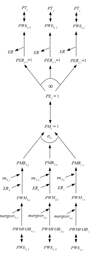
The price system for the Globe region is illustrated in Figure 3. On the import side Globe operates like all other regions. The commodities used in trade and transport services are assumed to be differentiated by source and aggregated using a CES and can potentially incur trade and transport margins (margcor) and face tariffs (tm); in fact the database does not include any transport margins or tariff data for margin services in relation to the destination region, although they can, and do, incur export taxes levied by the exporting region.

Therefore the average export price (PE) should equal the price paid by each destination region (PER) which should equal the export price in world currency units (PWE) and will be

common across all destinations (PT).

Figure 3 Price System for the Globe Region

∞

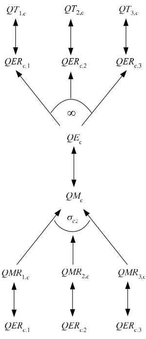
The linked quantity system contains the same asymmetry in the treatment of imports and exports by Globe, see Figure 4. The imports of trade and transport commodities are assumed to be differentiated by region of origin, hence the elasticity of substitution is greater than zero but less than infinity, while the exports of trade and transport commodities are assumed to be homogenous and hence the elasticities of transformation are infinite.

transport commodities exported to Globe; however the sum of Globe’s trade balances with other regions must be zero since Globe is a artificial construct rather than a real region. But the demand for trade and transport services by any region is determined by technology, i.e., the coefficients margcor, and the volume of imports demanded by the destination region. This means that the price of trade and transport commodities only have an indirect effect upon their demand – the only place these prices enter into the import decision as a variable is as a partial determinant of the difference between the fob and cif valuations of other imported

commodities. Consequently the primary market clearing mechanism for the Globe region comes through the quantity of trade and transport commodities it chooses to import.

Figure 4 Quantity System for the Globe Region

∞

4. FORMAL DESCRIPTION OF THE MODEL

This formal description of the model proceeds in four stages with three of them in this section and the fourth, relating to model closure rules, being detailed in the next section. For this section the description begins with identification of the sets used in the model, this is followed by details of each equation (block) in the model and ends with a table that summarises all the equations and identifies the associated variables, the counts for equations and variables and identifies whether the equation is implemented or not for the Globe region.

MODEL SETS

Rather than writing out each and every equation in detail it is useful to start by defining a series of sets; thereafter if a behavioural relationship applies to all members of a set an equation only needs to be specified once. The natural choice for this model is a set for all the transactions by each region (sac) plus a series of sets that group commodities, activities, factors, import duties, export taxes, trade margins, trade and finally some individual accounts relating to domestic institutions. The outer set for any region is defined as

{

}

sac= c a f hous tmr ter tff prodtax saltax dirtax govt kap owatpmarg w total

and the following are the basic sets for each region in this model

{

}

{

}

{

}

{

}

{

}

{

}

{

}

{

}

( ) commodities ( ) activities ( ) factors ( ) import duties ( ) export taxes ( ) factort taxes

( ) trade and transport margins ( ) rest of the world - trade

c sac

a sac

f sac

tmr sac

ter sac

tmr sac

owatpmarg sac

w sac

= = = = = = = =

{

}

{

}

{

}

{

}

{

}

( , ) trade margin commodities ( , ) non-trade margin commodities ( , ) export commodities

( , ) non-export commodities ( , , ) export commodities by region ( , , ) non-export commodities

ct c r

ctn c r

ce c r

cen c r

cer c r w

cern c r w

= = = = = =

{

}

{

}

{

}

{

}

{

}

{

}

( , ) non-imported commodities ( , , ) imported commodities by region ( , , ) non-imported commodities by region

( , ) commodities produced domestically

cm c r

cmn c r

cmr c r w

cmrn c r w

cx c r

cx = = = = =

{

}

{

}

{

}

( , ) commodities NOT produced domestically AND imported ( , ) commodities produced AND demanded domestically ( , ) commodities NOT produced AND demanded domestically ( , ) commodities WITH in

n c r

cd c r

cdn c r

cintd c r

= = =

=

{

}

{

}

termediate demand by region ( , ) commodities WITHOUT intermediate demand by region

cintdn c r =

It is also necessary to define a set of region, r, for which there are two subsets

{

}

{

}

2( ) all regions excluding Globe

( ) reference regions for global numeraire

r r

ref r

=

= .

A macro SAM that can be used to check various aspects of model calibration and operation is very useful. This needs another set

{

}

ss= commdty activity valuad hholds tmtax tetax govtn kapital margs,world totals

Reserved Names

The model uses a number of names that are reserved. The majorities of these reserved names relate to taxes and are reserved to ease the modeling of tax instruments; these are

DIRTAX Direct Taxes SALTAX Sales Taxes PRODTAX Production Taxes

FACTAX Factor Taxes

The other reserved name is for the capital/savings account. The reserved name is kap and this account handles all investment expenditures and savings.

Conventions

The equations for the model are set out in ten ‘blocks’; which group the equations under the following headings ‘exchange rates’, ‘trade’ – with sub blocks for ‘exports’ and ‘imports’, ‘commodity prices’, ‘numéraire’, ‘production’, ‘factors’, ‘household’, ‘government’ – with sub blocks for ‘taxes’ and ‘expenditure’, ‘kapital’ (savings and investment) and ‘market clearing’ – with various sub blocks for different dimensions of model closure. This grouping of equations is for ease of reading of the model rather than being a requirement of the model.

A series of conventions are adopted for the naming of variables and parameters. These conventions are not a requirement of the modeling language; rather they are designed to ease reading of the model.

̇ All VARIABLES are in upper case.

̇ The standard prefixes for variable names are: P for price variables, Q for quantity variables, W for factor prices, F for factor quantities, E for expenditure variables, Y for income variables, and V for value variables

̇ All variables have a matching parameter that identifies the value of the variable in the base period. These parameters are in upper case and carry a ‘0’ suffix, and are used to initialise variables.

̇ A series of variables are declared that allow for the equiproportionate adjustment of groups of parameters. These variables are named using the convention **ADJ, where ** is the parameter series they adjust.

̇ All parameters are in lower case, except those used to initialise variables.

̇ Names for parameters are derived using account abbreviations with the row account first and the column account second, e.g., actcom** is a parameter referring to the activity:commodity (supply or make) sub-matrix;

EQUATIONS FOR THE MODEL

The model equations are reported and described below and then they are summarised in Table4.

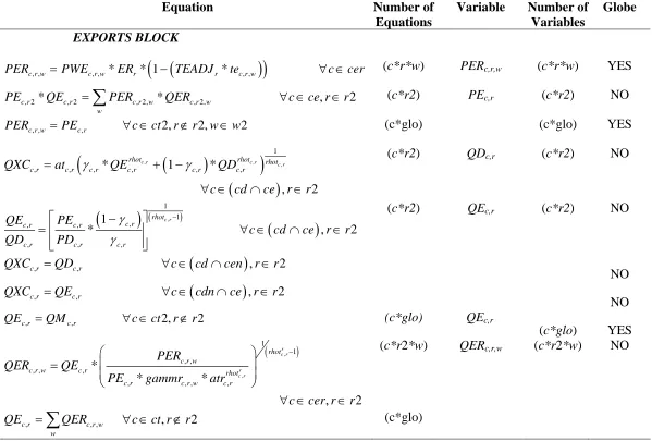
Exports Block Equations

The domestic prices of commodity exports, c, by destination, w, and source, r, region (PER) are defined as the product of world prices of exports (PWE) – also defined by commodity and destination and source region, the source region’s exchange rate (ER) and one minus the export subsidy rate5 (te) multiplied by a region specific export subsidy rate adjustment variable (TEADJ).

(

)

(

)

, , , , * * 1 * , ,

c r w c r w r r c r w

PER =PWE ER − TEADJ te ∀ ∈c cer

, 2

∀ ∈ ∈

∈

(X1) The possibility of non-traded commodities means that the equations for the domestic prices of

exports (and imports) are only implemented for those commodities that are traded; this requires the use of a dynamic set, cer, which is defined by those commodities that are exported in the base data. Also notice that the world prices of exports (PWE) are defined as variables; in a global model the small country trade assumption is not valid since, by definition, world prices are endogenous and therefore ALL regions are treated as ‘large’ producers of a commodity.

The prices of the composite export commodities can then be expressed as simple volume weighted averages of the of the export prices by region,

, * , , , * , ,

c r c r c r w c r w w

PE QE =

∑

where PEc,r and QEc,r the price and quantity of the composite export commodity c from region

r, and the weights are the volume shares of exports and are variable. This comes from the fact

that a CET function is liner homogenous and hence Eulers theorem can be applied. Notice however that (X2) is only implemented of the set r2, i.e., the region Globe is excluded. Rather the composite export price for trade margin commodities from Globe is given by

, , , 2, 2, 2

c r w c r

PER =PE ∀ ∈c ct r∉r w w (X3)

5

which indicates that it is assumed that the trade margin commodities exported by Globe are perfect substitutes for each other, i.e., the same price is paid for each trade margin commodity by ALL purchasing regions.

Domestic commodity outputs (QXC) are either exported (QE) as composite

commodities or supplied to the domestic market (QD). The allocation of output between the domestic and export markets is determined by the output transformation functions, Constant Elasticity of Transformation (CET) functions, (X4)

(

)

(

)

(

)

, , _,

1

, , , * , 1 , * ,

, 2

c r c r _{c r}

rhot rhot _rhot c r c r c r c r c r c r

QXC at QE QD

c cd ce r r

γ γ

= + −

∀ ∈ ∩ ∈

(X4)

with the optimum combinations of QE and QD determined by first-order conditions (X5)

(

)

(

)

c r c r c r

QE PE

c cd ce r r

QD PD γ γ − ⎡ − ⎤ =⎢ ⎥ ∀ ∈ ⎢ ⎥ ⎣ ⎦ 2

∩ ∈ . (X5)

However, some commodities are non-traded and therefore X4 and X5 are implemented if and only if the commodity is traded. This means that domestic commodity outputs are undefined for non-traded commodities, but by definition the quantity supplied to the domestic market is the amount produced, hence

(

)

, , ,

c r c r

QXC =QD ∀ ∈c cd∩cen r∈r2. (X6)

Furthermore it is necessary to cover the possibility that a commodity may be produced domestically and exported but not consumed domestically, hence

(

)

, , ,

c r c r

QXC =QE ∀ ∈c cdn∩ce r∈r2. (X7)

These quantity equations deal however only with the composite export commodities, i.e., hypothetical commodities whose roles in the model are to act as neutral intermediaries that enter into the first-order conditions that determine the optimal mix between domestic use and exports of domestic commodity production (X5). In fact the composite export

( , ) , 1 1 , , , , , , , , , * * * , 2 r c r r c r rhot c r w

c r w c r _rhot

c r c r w c r

PER QER QE

PE gammr atr

c cer r r

− ⎛ ⎞ ⎜ ⎟ = ⎜ ⎟ ⎝ ⎠ ∀ ∈ ∈ (X8)

for which the corresponding first order condition is given by (X2). Note however that (X8) does not define the exports of trade margin commodities BY Globe; this is because these commodities are assumed to be perfect substitutes and therefore simple addition is adequate, i.e.,

, , , ,

c r c r w w

QE =

∑

∉

. (X9)

Finally there is a need for an equilibrium conditions for trade by Globe. Since Globe is a artificial construct whose sole role in the model is to gather exports whose destinations are unknown and supply imports whose sources are unknown, and visa versa, it must always balance its trade within each period. Thus the volume exports of trade margin commodities by Globe must be exactly equal to the volume imports of trade margin commodities, i.e.,

, , 2, 2

c r c r

QE =QM ∀ ∈c ct r r . (X10)

Imports Block Equations

The prices of imported commodities are made up of several components. The export price in foreign currency units – valued free on board (fob) (PWMFOB) – plus the cost of trade and transport services, which gives the import price carriage insurance and freight (cif) paid (PWM), plus any import duties; all of which are then converted into domestic currency units (PMR). Clearly the import price values fob (PWMFOB) is identical to the export price valued fob (PWE) – this condition is imposed in the market clearing block (see below) – and hence the cif price can be defined as

, , , , , , , * ,

c r w c r w cp c r w cp r cp ct

PWM PWMFOB margcor PT

c cmr ∈ = + ∀ ∈

∑

trade and transport services or the quantity of services required to transport a particular commodity.

The domestic prices of imports from a region (PMR) are defined as the product of world prices of imports (PWM) – after payment for carriage, insurance and freight (cif) - the

exchange rate (ER) and one plus the import tariff rate (tm) multiplied by a tariff rate adjustment variable (TMADJ)

(

)

(

)

, , , , * * 1 * , ,

c r w c r w r r c r w

PMR PWM ER TMADJ tm

c cmr

= +

∀ ∈ . (M2)

The possibility of non-traded commodities means that the equations for the domestic prices of imports are only implemented for those commodities that are traded; this requires the use of a dynamic set, cmr, which is defined by those commodities that are imported by a region from another region in the base data. Also notice how the world prices of imports (PWM) are defined as variables.

The prices of the composite import commodities can then be expressed as simple volume weighted averages of the of the export prices by region,

, * , , , * , ,

c r c r c r w c r w w

PM QM =

∑

where PMc,r and QMc,r the price and quantity of the composite import commodity c by region

r, and the weights are the volume shares of imports and are variable. This comes from the fact

that a CES function is liner homogenous and hence Eulers theorem can be applied. Notice however that (M3) is only controlled by the set cm, in contrast to (X2) – the composite export price – which was also controlled by the set r2, i.e., the region Globe was excluded. This reflects the fact that the region Globe does import commodities using the same trading

assumption as other regions but only exports homogenous trade and transport services, which explains the need for the equation (X3).

(

)

(

)

(

)

, , _,

1

, , , * , 1 , * ,

, 2

c r c r _{c r}

rhoc rhoc _rhoc c r c r c r c r c r c r

QQ ac QM QD

c cx cm r r

δ δ ⎛ ⎞ −⎜ ⎟ − − ⎜_⎝ ⎟_⎠ = + − ∀ ∈ ∩ ∈ (M4)

with the optimal combinations of QM and QD being determined by first-order conditions, i.e.,

(

)

(

)

c r c r c r

QM PD

c cx cm r r

QD PM δ δ + ⎡ ⎤ =⎢ ⎥ ∀ ∈ − ⎢ ⎥

⎣ ⎦ ∩ ∈ 2

2

∈

2

∈

. (M5)

However, some commodities are non-traded and therefore M4 and M5 are implemented only if the commodity is traded. This leaves QQ undefined for non-traded commodities, but by definition the quantity demanded by the domestic market is the amount produced, hence

(

)

, , ,

c r c r

QQ =QD ∀ ∈c cx∩cmn r r . (M6)

Furthermore, it is necessary to cover the possibility that there is no domestic production of a commodity, hence

(

)

, , ,

c r c r

QQ =QM ∀ ∈c cxn∩cm r r . (M7)

The composite import commodities are defined as CES aggregates of the imports from different regions (QMR), i.e.,

( ) , , 1 1 , , , , , , , , , * * * r r

c r c r

rhoc rhoc c r w c r

c r w c r r

c r c r w

PMR acr

QMR QM c cmr

PM delta − + ⎛ ⎞ ⎜ ⎟ = ⎜ ⎟ ⎝ ⎠

∀ ∈ (M8)

where the first order conditions come from the price definition terms for composite imports,

PM (M2) and are only implemented for those cases where there were import transactions in

the base period – this is controlled by the set cmr. However also associated with any imported commodity is a specific quantity of trade and transport services. These services are assumed to be required in fixed quantities per unit of import by a specific region from another specific region, i.e.,

(

)

, , , , * , , ,

c r w cp r w c cp r w cp

QT =

∑

where the margcor are the trade and transport coefficients associated with a unit (quantity) import by region r from region w. This is only implemented for trade and transport

Commodity Price Block Equations

The composite price equations (CP1, CP2 and CP3) are derived from the first order

conditions for tangencies to consumption and production possibility frontiers. By exploiting Euler’s theorem for linearly homogeneous functions the composite prices can be expressed as expenditure identities rather than dual price equations for export transformation and import aggregation, such that PQS is the weighted average of the producer price of a commodity, when PD is the producer price of domestically produced commodities and PM the domestic price of the composite imported commodity, i.e.,

(

) (

)

(

)

, , * , , * ,

c r c r c r c r c r

PQS = PD QD + PM QM ∀ ∈c cd ∪cm ,r∈r2. (CP1) where QD the quantity of the domestic commodity demanded by domestic consumers, QM the quantity of composite imports and QQ the quantity of the composite commodity. Notice how the commodity quantities are the weights. This composite commodity price (CP1) does not include sales taxes, which create price wedges between the purchaser price of a

commodity (PQD) and the producer prices (PQS). Hence the purchaser price is defined as the producer price plus the sales taxes (CP2), i.e.,

(

)

(

)

(

)

, , * 1 * , , 2

c r c r r c r

PQD = PQS + TSADJ ts ∀ ∈c cd ∪cm r∈r . (CP2)

This formulation means that the sales taxes are levied on all sales on the domestic market, irrespective of the origin of the commodity concerned.

The composite output price for a commodity is also derived by exploiting Euler’s theorem for linearly homogeneous functions, and is given by

(

) (

)

,

* *

, 2

c r c r c ce r c ce r c r

c

PD QD PE QE

PXC

QXC

c cx r r

∈ ∈

+ =

∀ ∈ ∈

. (CP3)

Numéraire Price Block

It is also desirable to define a price numéraire for each region; for this model two alternative numéraire are defined so as to allow the modeler some discretion as to the choice of

numéraire. The consumer price indices (CPI) are defined as base weighted sum of the

commodity prices, where the weights are the value shares of each commodity in final demand (comtotshc), i.e.,

, * ,

r c r c r

c

CPI =

∑

2

∀ ∈

2

∀ ∈

. (N1)

The domestic producer price indices (PPI) are defined as the weighted sums of the commodity prices received by producers on the domestic market, where the weights are the value shares of each commodity supplied by domestic producers to the domestic market (vddtotshc), i.e.,

, * ,

r c r c r

c

PPI =

∑

This provides a convenient alternative price normalisation term; if the exchange rate is also fixed it serves to fix the real exchange rate.

Notice how both price indices are controlled to be implemented only for those regions that have consumption and production activities. Hence the Globe does not have its own price indices, rather the price indices for Globe are those of the reference region in the model.

Production Block Equations

The output price by activity (PX) is defined by the share of commodity outputs produced by each activity, as

, , , * ,

a r a c r c r c

PX =

∑

where, for this case, the weights (actcomactsh) are equal to one where the commodities and activities match and zero otherwise, i.e., there is a one to one mapping between the

commodity and activity accounts. The weights are derived from the information in the supply or make matrix.

payments for intermediate inputs and production taxes per unit of output (tx) multiplied by an indirect tax rate adjustment variable (TXADJ). The assumption of fixed proportions in the use of intermediate inputs, i.e., Leontief style input-output coefficients (comactco), means that the payments for intermediate inputs are the weighted sums of the intermediate input coefficients where the weights are the consumer prices of the composite commodities, i.e.,

(

)

(

)

(

)

, , * 1 * , , * ,

2

a r a r r a r c r c a r

c

PV PX TXADJ tx PQ comactco

r r ⎛ ⎞ = − _{− ⎜} ⎝ ∀ ∈

∑

⎠ . (P2)

The production sub-block consists of the production function (P3), a mapping of activity outputs (QXa) into commodity supplies (P6) and first order conditions for profit maximization

(P4). The specification for production uses CES production functions, which allows for elasticities of substitution other than unity. Again it is an aggregation function over the all factors that are demanded by each activity (FDf,a), where

, , 1 , , * , , * , , x a r x a r x

a r a r f a r f a r f

QX adces FD r r

ρ ρ δ − − ⎡ ⎤ = _{⎢ ⎥}

⎣

∑

with efficiency parameters (adcesa,r) and the factor shares ( , ,

x f a r

δ ) calibrated from the data and

the elasticities of substitution, from which the substitution parameters are derived (ρ_{a r}x_, ), exogenously imposed. The associated first-order conditions for optimal factor combinations are derived from equalities between the wage rates for each factor in each activity and the values of the marginal products of those factors in each activity, i.e.,

( ) , , , , , , 1 1 1 , , , , , , , , , , , , * * * * * * 2, x x

x a r

a r a r

f r f a r

x x

a r a r f a r f a r f a r f a r f

x f a r WF WFDIST

PV adces FD FD

r r ρ _ρ ρ δ δ δ ⎛⎛ ₋ ⎞ ⎞ ⎜⎜_⎜ ⎟−_⎟ ⎟ ⎜_{⎝ ⎠} ⎟ ⎝ ⎠ − − − ⎡ ⎤ = _{⎢ ⎥} ⎣ ⎦ ∀ ∈

∑

Since production uses intermediate inputs it is also necessary to specify the demand for intermediate inputs (QINTD). This is done from the perspective of commodity demands, i.e., it is summed over activities to produce the demand for intermediate inputs by commodity rather than by activity

, , , * , 2, int ???

c r c a r a r a

This is linked to the market clearing equation ??? below. Finally it is necessary to define the relationship between activity and commodity outputs, which is the counterpart to the price equation linking commodity and activity prices (P1). This is defined as a simple linear relationship whereby the commodity output is defined as the sum of the quantities of each commodity produced by each activity, i.e.,

, , , * ,

c r a c r a r a

QXC =

∑

2

∀ ∈

. (P6)

Factor Block Equations

The total income received by each factor account (YFf) is defined as the summation of the

earnings of that factor across all activities (F1),

, , * , , * , ,

f r f r f a r f a r a

YF =

∑

Only a proportion of total factor income is available for distribution to the domestic institutional accounts. First allowance must be made for depreciation, which it is assumed takes place at fixed rates (deprecf,r) relative to factor incomes and the payment of factor

income taxes (tyff,r) that are assumed to be simple average ad valorem rates but with the

option of an adjustment factor (TYFADJ), i.e.,

(

)

(

)

(

(

)

)

, , , * , * 1 *

2

f r f r f r f r r f r

YFDIST YF deprec YF TYFADJ tyf

r r

= − − _,

∀ ∈ . (F2)

Although implemented over all factors, this equation is only relevant in this model for income to the factor capital.

Household Block Equations

Households acquire income from only one source in this model; the sale of factor services. Therefore household income (YH) is defined as

, , 2

h r f r

f

YH =

∑

(

)

(

)

(

)

(

)

(

)

* 1 *

* 1 * 2

h r h r r h r

r h r

HEXP YH TYHADJ tyh

SADJ kaphsh r r

= −

− ∀ ∈ (H2)

Note how the saving rates are defined as proportions of after tax incomes that are saved; this is important for the calibration of the income tax and savings parameters. The quantities of each commodity demanded by the household are then defined by the shares of household consumption expenditure (comhoav) divided by the consumer price of the specific commodity (H3). This is a specification for a Cobb-Douglas utility function, i.e.,

, , ,

,

,

*

2

c h r h r h

c r

c r

comhoav HEXP

QCD r r

PQ

⎛ ⎞

⎜ ⎟

⎝ ⎠

=

∑

One advantage of the Cobb-Douglas specification is that it results in the changes in the values for household consumption expenditures (HEXP) being equal to the changes in an equivalent variation measure of household welfare.

Government Tax Block Equations

There are six tax instruments. Each is defined as a simple ad valorem rate dependent upon the values of imports, exports, sales or production and the levels of factor and household and income. The ‘tax’ rates are all declared as parameters and then for each tax instrument a scaling variable is declared to facilitate policy experiments. Import duties (MTAX) are defined as

(

)

2

r r c r w c r w r c r w

w c

MTAX TMADJ tm PWM ER QMR

r r

=

∀ ∈

∑∑

(T1)

where tm is the tariff rate and TMADJ the scaling variable. Export taxes (ETAX) are defined as

(

)

2 r r c r w c r w r c r w

w c

ETAX TEADJ te PWE ER QER

r r

=

∀ ∈

∑∑

(T2)

(

)

* *

2 *

r c r c r

r

c c r c r c r c r

TSADJ ts PQ

STAX r r

QINTD QCD QGD QINVD

⎛ ⎞ = _⎜⎜ ∀ + + + ⎝ ⎠

∑

)

where ts is the sales tax rate and TSADJ the scaling variable. Indirect/production taxes (ITAX) are defined as

(

r r a r a r a r

a

ITAX =

∑

where tx is the indirect tax rate and TXADJ the scaling variable. Factor income taxes (FTAX) are defined as

(

)

(

)

(

)

2

r r f r f r f r f r

f

FTAX TYFADJ tyf YF deprec YF

r r

= −

∀ ∈

∑

(T5)

where tyf is the factor income tax rate and TYFADJ the scaling variable. Household income taxes (DTAX) are defined as

(

)

r r h r h r

h

2

HTAX =

∑

r

(T)

where tyh is the household income tax rate and TYHADJ the scaling variable.

Government Block Equations

Government income (YG) is defined as the sum of government tax revenues (G1), i.e.,

2

r r r r r r

YG MTAX ETAX STAX ITAX FTAX HTAX r r

= + + + + +

∀ ∈ . (G1)

The tax revenues are treated as expenditures by the accounts paying the taxes and hence are defined in the tax block. Although this approach adds equations it has the arguable advantage of being more transparent and easier to modify.

Government demand for commodities (G2) is assumed fixed in real terms, i.e., the volume is fixed, but can be scaled or allowed to vary using an adjustment factor (QGDADJ). The precise specification depends upon the choice of closure rule (see below).

, , *

c r c r r

QGD =comgovconst QGDADJ ∀ ∈r r2. (G2)

, * ,

r c r c r c

EG =

∑

,

h r

2

∀ ∈

2

. (G3)

Kapital Account Block Equations

Income to the capital (savings and investment) account comes from household savings, depreciation allowances, government savings (KAPGOV) and the surplus on the capital account of the balance of payments (KAPWOR) (K1). Hence total savings are defined as

(

)

(

)

(

)

(

)

(

)

, ,

, ,

* 1 * * *

*

* 2

r h r r h r r

h

f r f r f

r r r

TOTSAV YH TYHADJ tyh SADJ kaphsh

deprec YF

KAPGOV KAPWOR ER r r

⎛ ⎞

=_⎜ − _⎟

⎝ ⎠

+

+ + ∀ ∈

∑

∑

In this model the household is assumed to save fixed proportions (kaphsh) of their income after tax. Both the household savings and income tax rates are multiplied by adjustment variables (SADJ and TYHADJ). The savings rate adjustment variable means savings rates can adjust to achieve an exogenously defined level of total savings if an investment driven closure rule is assumed. It may be helpful to assign (K1) simultaneously with (H2) to ensure correct calibration of the income tax and saving rate parameters. Government savings are calculated as residual (see the KAPGOV equations below): note that the surplus on the capital account (KAPWOR) is defined in terms of the foreign currency and therefore the exchange rate appears in this equation (this is a matter of preference).

Investment demand is modeled in a similar way to government demand. Demand for commodities (K2) used in investment is assumed to be in fixed volumes (invconst) multiplied by an investment-scaling variable (IADJ) that can accommodate changes in the exogenously determined level of investment and/or changes in the availability of funds for investment, i.e.,

, * ,

c r r c r

QINVD =IADJ invconst r r . (K2)

The second stage (K3) captures the price effect by identifying the total value of investment (INVEST), i.e.,

(

)

r c r c r

c

Market Clearing Block Equations

The market clearing, or equilibrium, conditions are straightforward. Factor supplies must equal factor demands (MC1)

, , , 2

f r f a r a

FS =

∑

∈

∈

(MC1)

and (composite) commodity supplies must equal (composite) commodity demands (MC2)

(

)

, , , , ,

, 2

c r c r c r c r c r

QQ QINTD QCD QGD QINVD

c cd cm r r

= + + +

∀ ∈ ∪ ∈ . (MC2)

It appears that there is no equilibrium condition for the supply of domestic output to the domestic market. In fact this is achieved through the commodity output equation (P5), which could have been treated as a market clearing equation.

The government account is cleared by defining government savings (KAPGOV) as the difference between government income and government expenditure on consumption and transfers, hence government savings are explicitly treated as a residual, i.e.,

2

r r r

KAPGOV =YG −EG ∀ ∈r r . (MC3)

The deficit on the current account is computed in two-stages. First the bilateral trade balances (KAPREG) are calculated as the difference in the values of imports and exports – for convenience theses are evaluated in the currency of the reference region, i.e.,

, , , , ,

, , , ,

*

* 2

r w c r w c r w c

c r w c r w c

KAPREG PWM QMR

PWE QER r r

⎛ ⎞ = ⎜ ⎟ ⎝ ⎠ ⎛ ⎞ −_{⎜ ⎟} ∀ ⎝ ⎠

∑

∑

and then the overall balance of trade (KAPWOR) is computed for each region, i.e.,

2 , 2, , 2,

, 2, , 2,

*

* 2

r c r w c r w

w c

c r w c r w w c

KAPWOR PWM QMR

PWE QER r r

⎛ ⎞ = ⎜_⎝ ⎟_⎠ ⎛ ⎞ −_{⎜ ⎟} ∀ ⎝ ⎠

∑∑

∑∑

transactions and these are equated in both value and quantity terms. Also because (MC5) is defined in terms of the ‘foreign’ currency it is necessary to convert KAPWOR into domestic currency terms when it enters into any other equation, e.g., the total savings equation (TOTSAV).

The next pairs of market clearing conditions relate to trade in commodities. The first set trade consistency conditions (TRCONP) deal with the fob prices of imports and exports; by definition these must be identical and hence

, , , ,

c r w c rp wp

PWMFOB =PWE ∀ ∈c cmr

∈ ∈

∈

. (MC6) These equations are not completely straightforward since it is necessary in their

implementation to employ mappings between exporting and importing regions that require the ‘switching’ of labels on accounts within the equation. The second set trade consistency

conditions (TRCONQ) deal with the quantities of imports and exports; by definition these must be identical and hence

, , , ,

c r w c rp wp

QMR =QER ∀ ∈c cmr (MC7)

again these equations are not completely straightforward since it is necessary in their implementation to employ mappings between exporting and importing regions.

The trade consistency equations do not however deal with the requirements for market clearing with respect to the trade transactions undertaken by the Globe region. These require that the total demand for each and every trade and transport service (QT) is exactly equal to the exports of that service by Globe, i.e.,

, , , , 2, 2

c r w c r w w

QT =QER ∀c ct r r

∑

And second that the export price of each and every trade and transport margin service is identical irrespective of the region that is importing the service. i.e.,

, , , 2, 2

c r c r w

PT =PWE ∀ ∈c ct r r (MC9)

which embodies the presumption that trade and transports services of each type are identical irrespective of who supplies or purchases them.

2

r r r

TOTSAV =INVEST +WALRAS ∀ ∈r r

r r

KAPWORSYS = KAPWOR

where KAPWORSYS is fixed at zero.

also includes a slack variable, rather than dropping an equation from the system (MC10). And second there is a market clearing condition on the relationship between each regions’ trade balance, i.e.,

∑