Analysis of Connecting Rod Bearing Design Trends Using a Mode-Based Elastohydrodynamic Lubrication Model

Rochester Institute of Technology

RIT Scholar Works

Theses

Thesis/Dissertation Collections

8-8-2013

Analysis of Connecting Rod Bearing Design

Trends Using a Mode-Based Elastohydrodynamic

Lubrication Model

Travis M. Blais

Follow this and additional works at:

http://scholarworks.rit.edu/theses

Part of the

Acoustics, Dynamics, and Controls Commons

This Thesis is brought to you for free and open access by the Thesis/Dissertation Collections at RIT Scholar Works. It has been accepted for inclusion in Theses by an authorized administrator of RIT Scholar Works. For more information, please contactritscholarworks@rit.edu.

Recommended Citation

Analysis of Connecting Rod Bearing Design Trends Using a

Mode-Based Elastohydrodynamic Lubrication Model

By

Travis M. Blais

A Thesis Submitted in Partial

Fulfillment of the Requirements for the Degree of

MASTERS OF SCIENCE

IN

MECHANICAL ENGINEERING

Approved:

August 8, 2013

DEPARTMENT OF MECHANICAL ENGINEERING

KATE GLEASON COLLEGE OF ENGINEERING

Committee Approval

Dr. Stephen Boedo

Signature: ______________________

Associate Professor, Thesis Advisor

Date: ______________________

Department of Mechanical Engineering

Dr. Jason Kolodziej

Signature: ______________________

Assistant Professor

Date: ______________________

Department of Mechanical Engineering

Dr. Alexander Liberson

Signature: ______________________

Visiting Associate Professor

Date: ______________________

Department of Mechanical Engineering

Dr. Agamemnon Crassidis

Signature: ______________________

Associate Professor

Date: ______________________

Department of Mechanical Engineering

i

Abstract

Available design trends for big end connecting rod bearings utilize widely adopted rapid methods for prediction of minimum film thickness due to their superior speed and ease of use. However, they impose unrealistic assumptions such as surface rigidity, which could compromise the accuracy of results. The significance of structural elasticity and updated models was investigated using a mode based

elastohydrodynamic lubrication model which includes body forces, mass conserving cavitation, and surface roughness. Eight physical connecting rods were modeled using finite element methods and simulated over a variety of conditions, varying engine speed, bearing clearance, and oil viscosity. The results show operating conditions where rapid methods can inaccurately predict minimum film thickness. Bearings operating at higher speeds and loads are subject to significant bearing deformation that

ii

Acknowledgements

iii

Table of Contents

Chapter 1: Introduction ... 1

1.1 The Mobility Method ... 3

1.2 Mode Based Elastohydrodynamic Method ... 5

Chapter 2: Problem Formulation ... 7

2.1 Bearing Duty ... 7

2.2 Mode Based Elastohydrodynamic Model ... 11

2.3 Modeling Process and Procedure ... 13

Chapter 3: Model Validation ... 16

3.1 Introduction ... 16

3.2 Modal Accuracy ... 16

3.3 Nodal Validation ... 22

3.4 Mesh Density and Modal Inclusion ... 27

3.5 Experimental Validation ... 38

Chapter 4: Implementation of Mode Based EHD ... 42

4.1 Introduction ... 42

4.2 Connecting Rod Models... 43

4.3 Speed Variation Study ... 51

4.3.1. Bearing Duty ... 51

4.3.2. Minimum Film Thickness Results ... 54

4.3.3. Discussion ... 66

4.4 Clearance Variation Study ... 71

4.4.1. Bearing Duty ... 71

4.4.2. Minimum Film Thickness Results ... 71

4.4.3. Discussion ... 83

4.5 Viscosity Variation Study ... 86

4.5.1. Bearing Duty ... 86

4.5.2. Minimum Film Thickness Results ... 86

iv

4.6 Parametric Study ... 98

4.6.1. Results ... 98

4.6.2. Discussion ... 107

v

List of Tables

Table 3.1: General Motors connecting rod specifications ... 17

Table 3.2: General Motors eigenvalue comparison ... 18

Table 3.3: General Motors mode shape correlation coefficient ... 21

Table 3.4: Design0 bearing and operational parameters ... 23

Table 3.5: Design0 mode shape correlation coefficients with 200x10 reference mesh ... 28

Table 3.6: Plain bearing physical and operational parameters... 39

Table 4.1: Connecting rod specifications ... 45

Table 4.2: Connecting rod eigenvalues ... 46

Table 4.3: Modeshape correlation coefficient compared to General Motors connecting rod. ... 49

Table 4.4: Speed variation specific parameters... 54

Table 4.5: Varied crankshaft speed values for given load factors ... 55

Table 4.6: Clearance variation specific parameters ... 71

Table 4.7: Varied radial clearance for given load factors ... 72

Table 4.8: Viscosity variation specific parameters ... 86

vi

List of Figures

Figure 1.1: Crankshaft, connecting rod, and piston assembly ... 1

Figure 1.2: Booker big-end connecting rod bearing design chart [2] ... 2

Figure 1.3: Journal bearing coordinate system geometry ... 3

Figure 1.4: Finite element mobility based design chart for [7] ... 5

Figure 2.1: Connecting Rod Geometry ... 7

Figure 2.2: Dynamic equivalent connecting rod mass model ... 9

Figure 2.3: Connecting rod free body diagram ... 10

Figure 2.4: Forces and Displacements ... 11

Figure 2.5: Preprocessing flowchart ... 14

Figure 2.6: EHD simulation flowchart ... 15

Figure 3.1: General Motors connecting rod meshed (Left: Published, Right: New) ... 17

Figure 3.2: General Motors modeshape comparison ... 19

Figure 3.3: Oh and Goenka Design0 connecting rod dimensions ... 23

Figure 3.4: Design0 load diagram ... 24

Figure 3.5: Design0 connecting rod with 48x10 surface mesh (Left) Original (Right) New ... 24

Figure 3.6: 48x5 and Published Minimum Film Thickness ... 25

Figure 3.7: 48x5 and Published Maximum Film Pressure ... 25

Figure 3.8: Design0 48x5 Minimum Film Thickness, Maximum Film Pressure 2 to 13 Modes ... 29

Figure 3.9: Design0 80x6 Minimum Film Thickness, Maximum Film Pressure 2 to 13 Modes ... 30

Figure 3.10: Design0 160x8 Minimum Film Thickness, Maximum Film Pressure 2 to 13 Modes... 31

Figure 3.11: Design0 200x10 Minimum Film Thickness, Maximum Film Pressure 2 to 13 Modes... 32

Figure 3.12: Design0 2 Mode Minimum Film Thickness, Maximum Film Pressure ... 34

Figure 3.13: Design0 7 Mode Minimum Film Thickness, Maximum Film Pressure ... 35

Figure 3.14: Design0 9 Mode Minimum Film Thickness, Maximum Film Pressure ... 36

Figure 3.15: Design0 13 Mode Minimum Film Thickness, Maximum Film Pressure ... 37

Figure 3.16: Experimental fixture ... 38

Figure 3.17: 2000N 2000RPM mid plane film pressure distribution ... 40

Figure 3.18: 6000N 2000RPM mid plane film pressure distribution ... 40

Figure 3.19: 10,000N 2000RPM mid plane film pressure distribution ... 41

vii

Figure 4.2: Connecting rod CAD half models (a) Alfa Carrillo (b) Alfa Stock (c) Datsun (d) FSAE (e)

General Motors (f) Mercedes (g) Porsche Carrillo (h) Volkswagen ... 44

Figure 4.3: Connecting rod modeshapes ... 47

Figure 4.4: Connecting rod modeshapes ... 48

Figure 4.5: Normalized cylinder pressure ... 52

Figure 4.6: Alfa Carrillo Bearing Load, Fpist/Frot = 0, Mrec/Mrot = 1, Load Factor = 0.1 ... 52

Figure 4.7: Alfa Carrillo Bearing Load, Fpist/Frot = 0, Mrec/Mrot = 1, Load Factor = 1 ... 53

Figure 4.8: Alfa Carrillo Bearing Load, Fpist/Frot = 5, Mrec/Mrot = 1, Load Factor = 0.1 ... 53

Figure 4.9: Alfa Carrillo Bearing Load, Fpist/Frot = 5, Mrec/Mrot = 1, Load Factor = 1 ... 53

Figure 4.10: Alfa Carrillo speed variation minimum film thickness ... 56

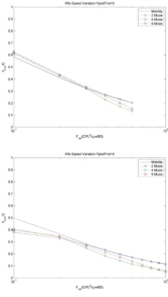
Figure 4.11: Alfa speed variation minimum film thickness ... 57

Figure 4.12: Datsun speed variation minimum film thickness ... 58

Figure 4.13: Formula SAE speed variation minimum film thickness ... 59

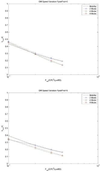
Figure 4.14: General Motors speed variation minimum film thickness ... 60

Figure 4.15: Mercedes speed variation minimum film thickness ... 61

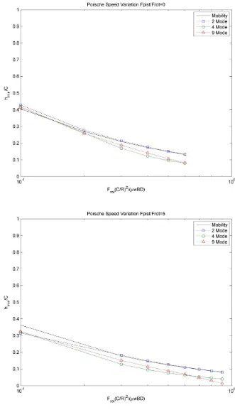
Figure 4.16: Porsche speed variation minimum film thickness ... 62

Figure 4.17: VW speed variation minimum film thickness ... 63

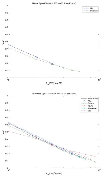
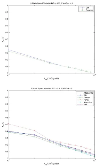
Figure 4.18: Speed variation connecting rod grouping Fpist/Frot=0 ... 64

Figure 4.19: Speed variation connecting rod grouping Fpist/Frot=5 ... 65

Figure 4.20: Volkswagen minimum film thickness history Fpist/Frot=0, Load Factor = 0.8 ... 67

Figure 4.21: Volkswagen film thickness distribution Fpist/Frot=0, Load Factor = 0.8 ... 67

Figure 4.22: Volkswagen film pressure distribution Fpist/Frot=0, Load Factor = 0.8 ... 68

Figure 4.23: Volkswagen minimum film thickness history Fpist/Frot=5, Load Factor = 1.0 ... 68

Figure 4.24: Volkswagen film thickness distribution Fpist/Frot=5, Load Factor = 1.0 ... 69

Figure 4.25: Volkswagen film pressure distribution Fpist/Frot=5, Load Factor = 1.0 ... 69

Figure 4.26: Alfa Carrillo clearance variation minimum film thickness ... 73

Figure 4.27: Alfa clearance variation minimum film thickness ... 74

Figure 4.28: Datsun clearance variation minimum film thickness... 75

Figure 4.29: FSAE clearance variation minimum film thickness ... 76

Figure 4.30: General Motors clearance variation minimum film thickness ... 77

Figure 4.31: Mercedes clearance variation minimum film thickness ... 78

Figure 4.32: Porsche clearance variation minimum film thickness ... 79

Figure 4.33: Volkswagen clearance variation minimum film thickness ... 80

viii

Figure 4.35: Clearance variation connecting rod grouping Fpist/Frot=5 ... 82

Figure 4.36: Alfa Carrillo film history, load factor = 0.1, Fpist/Frot = 5 ... 84

Figure 4.37: Alfa Carrillo pressure distribution, no oil feed and quasi static cavitation ... 85

Figure 4.38: Alfa Carrillo pressure distribution, oil feed and mass conserving cavitation ... 85

Figure 4.39: Alfa Carrillo viscosity variation minimum film thickness ... 88

Figure 4.40: Alfa viscosity variation minimum film thickness ... 89

Figure 4.41: Datsun viscosity variation minimum film thickness ... 90

Figure 4.42: FSAE viscosity variation minimum film thickness ... 91

Figure 4.43: General Motors viscosity variation minimum film thickness... 92

Figure 4.44: Mercedes viscosity variation minimum film thickness ... 93

Figure 4.45: Porsche viscosity variation minimum film thickness ... 94

Figure 4.46: Volkswagen viscosity variation minimum film thickness ... 95

Figure 4.47: Viscosity variation connecting rod grouping Fpist/Frot=0 ... 96

Figure 4.48: Viscosity variation connecting rod grouping Fpist/Frot=5 ... 97

Figure 4.49: Alfa Carrillo parametric comparison ... 99

Figure 4.50: Alfa parametric comparison ... 100

Figure 4.51: Datsun parametric comparison ... 101

Figure 4.52: FSAE parametric comparison ... 102

Figure 4.53: General Motors parametric comparison ... 103

Figure 4.54: Mercedes parametric comparison ... 104

Figure 4.55: Porsche parametric comparison ... 105

Figure 4.56: Volkswagen parametric comparison ... 106

Figure 4.57: Speed variation study load components and magnitude ... 108

Figure 4.58: Clearance variation study load components and magnitude... 108

ix

List of Symbols

Acyl piston cross sectional area m 2

B bearing length m C journal radial clearance m D bearing diameter m F journal load N Frec reciprocating force N

Fpist Piston gas force N

Frot rotational force N

Jr residual inertia kg-m 2

J polar moment of inertia kg-m2 L bearing length m L connecting rod center to center length m M mobility vector -

M mass kg

Mb big end mass kg

Ms small end mass kg

Mrot rotating mass kg

Mpist piston mass kg

Mrec reciprocating mass kg

Psup supply pressure Pa

Pcav cavitation pressure Pa

Pcyl cylinder pressure Pa

Pcyl* peak cylinder pressure Pa

R bearing radius m r crank radius m s crank to piston length m Tres residual torque N-m

ω engine rotational speed rad-s-1 Xcm center of mass m

x

{r} internal force vector N [T] transformation matrix - {v} velocity vector m-s-1 α x-direction eccentricity - β feed hole angle Degrees ϒ y-direction eccentricity - Є eccentricity - µ kinematic oil viscosity N-m-2-s θ crank angle Degrees

ϕ connecting rod angle Degrees

ϕ normalized displacement at test mode -

ρ fluid density kg-m-3

1

Chapter 1:

Introduction

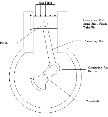
Dynamically loaded journal bearings are commonly encountered on machinery where a connection must support high loads and allow rotation. A particularly complex application is their use in reciprocating four stroke gasoline engines as connecting rod big-end bearings. The connecting rod serves as a linkage between the crankshaft and a piston as illustrated in Figure 1.1. Since the connecting rod is continually rotating and translating it experiences both high inertial loads and compressive forces from piston gas pressure.

Figure 1.1: Crankshaft, connecting rod, and piston assembly

Proper design is essential to avoid material wear and reduce friction through the use of a thin lubricant film. Solution methods range from the highly efficient mobility method to a complete finite element solution based on the Reynolds equation. Each offers a certain tradeoff between accuracy of results, and computational intensity.

2

Figure 1.2: Booker big-end connecting rod bearing design chart [2]

As computer capabilities increased so did the potential solution methods leading into complete finite element based solutions. Elastohydrodynamic (EHD) lubrication models were developed which can handle complex geometry, and bearing elasticity. However, the solutions are much slower than mobility based solutions, and the required software is generally unavailable to the practicing engineer. A historical overview of EHD methods which can be applied to problems such as connecting rods was developed by Booker et al [3].

A modal EHD solution was introduced by Kumar, Booker, and Goenka [4]. The modal approach represents bearing deformation by a combination of generalized displacements known as modes. It utilizes finite element methods to compute fluid flow and pressure. The mode-based method can model both bearing irregularities including oil feed holes, and bearing elasticity. Computationally more efficient than previously developed EHD solutions, the implementation is still complex in nature requiring

sophisticated tools to analyze bearing performance.

3

1.1 The Mobility Method

The mobility method serves as a benchmark for a rapid method to predict journal bearing

behavior. The essence of the mobility method is it relates journal translational velocity ( ̇) to journal load (F) through the use of a non-dimensional mobility map (M). For non-rotating journal bearings, the journal velocity is given by

{ ̇ ̇ }

| | {

⁄

⁄ }

(1.1)

where and are coordinate directions attached to the load vector as shown in Figure 1.3, C is the journal radial clearance, L is the bearing length, is the journal eccentricity ratio, R is the bearing radius, D is the bearing diameter, and is the kinematic fluid viscosity.

Figure 1.3: Journal bearing coordinate system geometry

Applying the mobility method to the general case of a rotating journal and sleeve is given by Equation (1.2). Journal translational velocity as expressed in an x,y computation frame is given by

{ ̇ ̇ } | | { ⁄ ⁄ } ̅ [

_{] [ ]}

(1.2)

where ̅ is the average angular velocity of the journal and sleeve. The mobility vector is calculated in the , map frame and transformed to the computing frame. Computational details can be found in Booker [5].

4

bearing length, bearing radius, and bearing clearance (Figure 1.2). The developed design chart is significant for its extensive study of dynamically loaded journal bearings as they apply to connecting rods. The chart is computed from 120 different simulations, loaded only by inertial forces due to rotation and reciprocating action. Most importantly it allows for prediction of minimum film thickness through simple algebraic relations and no simulation.

Although the described method is very computationally efficient, its weakness lies with its assumptions. The mobility map used for the design chart represented in Figure 1.2 is based off a short bearing approximation which neglects circumferential pressure flow. The method also assumes that half of the fluid always has a positive film pressure, while the other half is set to zero (ambient) pressure. The justification being that lubricant films cannot support negative film pressures; the fluid ruptures and undergoes cavitation causing a sub-ambient pressure condition. Another assumption is that loading due to gas forces does not have an effect on the bearing orbit as long as it is less than approximately seven times the inertial loading on the bearing. This means the solution is only valid when loading due to cylinder pressure is less than or equal to seven times inertial loading. The method does not take into account any structural deformation, which in many instances may be on the order of magnitude of the fluid film lubrication. It also only applies for groove-less bearings with circumferential symmetry and no oil feed. All of these assumptions suggest tremendous room for improvement and research based on today’s more realistic models.

The finite element derived mobility map created by Goenka [6] partially addressed some of the limitations of the short bearing model. Primarily the solution uses a finite length bearing in place of the short bearing approximation. The finite element based mobility method was applied to big-end connecting rod bearings by Boedo [7] to create design charts for cyclic minimum film thickness. The design charts represent hundreds of simulations using Goenka mobility map. The charts also consider cylinder pressure bearing loading unlike previous design charts. The published design charts represent the most complete rapid method solutions for big-end connecting rod bearings. However, the solutions still lack

5

Figure 1.4: Finite element mobility based design chart for [7]

1.2 Mode Based Elastohydrodynamic Method

Implementation of a mode based approach for EHD bearing analysis was first introduced by Kumar, Booker, and Goenka [4]. It was developed as a means to reduce the computational cost of bearing analysis where structural deformation may be important. The method offered increased speed and stability compared to conventional nodal EHD methods (which track thousands of surface locations) as well as improved accuracy from the mobility method. Mode based EHD lubrication models use a linear combination of eigenvectors (refered to as modes or mode shapes) and their respective eigenvalues to describe nodal displacements.

6

Later, Kumar, Goenka, and Booker [10] applied the modal method to a dynamically loaded automotive connecting rod model. The modal results using their computer code MODEHD, were

compared to the nodal results using a computer code developed by Oh and Goenka [8] named DEHD. At the time, DEHD was considered to be one of the most robust and accurate methods. For the same problem the MODEHD used one eighth of the computing cost. Moreover, with only eight modes it accurately agreed with DEHD results.

Continuing with developments, Boedo, Booker, and Wilkie [11] introduced a mass conserving cavitation model coupled with the modal EHD. Later that year Boedo added both body forces and surface roughness [12, 13]. The mass conserving cavitation model had originally been developed by Kumar and Booker [14], but was not coupled with modal EHD. The cavitation model tracks fluid density to more accurately predict oil flow. With the addition of the mass conserving cavitation model, predictions in general seemed to have thinner films and higher film pressures. The addition of structural inertia to transient modal EHD problems proved to be important for higher engine speeds. Surface roughness was modeled using pressure and shear flow factors from Patir and Cheng’s work [15]. An average Reynolds equation is used in which the pressure and shear flow factors are computed from numerical flow simulations. The implementation of surface roughtness showed little effect on bearing performance compared to past additions. Regardless, the model became more representative of real conditions.

7

Chapter 2:

Problem Formulation

2.1 Bearing Duty

The process of analyzing journal bearings can be split up into two main components. First is to compute the loads exerted on the bearing. Second is to then apply the loads to a journal bearing model, such as the mobility method, nodal, or modal EHD models. Focusing on the first, Figure 1.1 provides an overview of the basic engine composition. In the analysis that follows, it is assumed that the piston is constrained by the cylinder walls, and the crankshaft, connecting rod, and piston are all rigid. All bearings are treated as ideal pin joints for the computation of bearings loads. Additionally, it is assumed that the engine undergoes quasi steady state operation in the sense that it will only operate at a range of constant angular velocities at which there are no fluctuations or acceleration in the crankshaft angular velocity. External actions on the system are provided by cylinder gas forces and an external torque on the crankshaft. The external torque is required to maintain constant angular velocity.

Much of what follows is taken from Boedo [7] and Boedo and Booker [20] and is provided here for completeness.

Calculation of bearing loads is based on rigid body kinematics, where the rigid bodies are composed of crank radius r, and connecting rod center to center length L. Figure 2.1 shows the relationship between the components and three coordinate systems. The block frame, represented by and , is a fixed coordinate system with its origin at the crankshaft center of rotation. The crankshaft frame, represented by and , shares its origin with the block frame and rotates with the crankshaft vector r. Additionally, the connecting rod frame, and , rotates with vector ⃗ .

8

Vectors , ⃗ and are described by Equations (2.1) to (2.3) respectively:

̂ ̂

(2.1)

⃗ ̂ ̂

(2.2)

̂ ̂

(2.3)

Vector ⃗ is also defined by the addition of vectors and ⃗ shown by Equation (2.4). Combined with equations (2.1) to (2.3) useful expressions (2.5) and (2.6) can be found.

⃗

(2.4)

(2.5)

(2.6)

Differentiating (2.4) yields expressions (2.7) and (2.8) where

and since the bearing will

be evaluated for constant engine speeds.

(2.7)

(2.8)

9

the same, and the mass of the connecting rod is split into big end mass Mb and small end mass Ms based

on the connecting rod center of mass location Xcm. A massless residual inertia Jr is placed on the model so

that the moment of inertia of model and actual connecting rods are the same.

Figure 2.2: Dynamic equivalent connecting rod mass model

(2.9)

10

(2.11)

The free body diagram for the connecting rod is outlined in Figure 2.3. The force of interest is annotated as ⃗⃗⃗ which is the force from the journal to the big end sleeve.

Figure 2.3: Connecting rod free body diagram

The components of ⃗⃗⃗ can be solved for in the block frame and are given by equations (2.12) and (2.13). Transformations into crank and rod frames are given by (2.14) and (2.15) respectively, where Mrec = Ms +

Mpist and Mrot = Mb.

(2.12)

(2.13)

{ }

11

{ }

(2.15)

The journal and sleeve angular velocities also depend on the desired coordinate frame. Angular velocity for the block, crank and connecting rod frame respectively are as follows:

Although the choice of reference frame will not affect minimum film thickness results, forces are typically computed in the rod frame, for node and mode based EHD.

2.2 Mode Based Elastohydrodynamic Model

The mode based EHD lubrication model used throughout this work is the direct application of the model outlined by Boedo and Booker [16, 19, 20] which includes mass conserving cavitation, body forces, and surface roughness. The forces and displacements can be seen in Figure 2.4.

12

The relative displacement vector { }, defined by the difference between sleeve deformation and journal movement, can be represented by considering the connecting rod bearing stiffness matrix , elastic equilibrium matrix , external force vector { } and internal force vector { }.

{ } { } { }

(2.16)

In a similar fashion internal force vector { } can be related to hydrodynamic damping matrix , journal velocity vector { }, and residual force vector { }.

{ } { } { }

(2.17)

Coupling the relations yields the elastohydrodynamic nodal solution. Where n is the number of nodes and the vectors are of length n, and the matrices are of height and width n. Solving every iteration in time creates a very slow process. Therefore the modal solution transforms the vectors and matrices to size m, where m<<n, with transformation matrix .

{ } { }

(2.18)

{

}

{ }

(2.19)

(2.20)

(2.21)

(2.22)

{

}

{ }

(2.23)

The transformation matrix is a chosen set of relations represented by a set of eigenvectors from the generalized eigenvalue problem given by:

13

where [A] is the area matrix of the surface mesh. The mode based EHD solution is represented in terms of the transformed matrices as follows.

{ } { } {

} { }

(2.25

From the first implementation by Kumar [4], major improvements have been made to account for mass conserving cavitation [14, 21] and inclusion of body forces and surface roughness [12]. Mass conserving cavitation tracks fluid density in areas of ruptured fluid, so that fluid flow is correctly predicted.

Further improvements were made with the addition of body forces for the EHD approach. The effects of structural inertia and surface roughness was studied, and results shows that the addition of body forces on big-end connecting rod bearings has a significant influence on bearing performance. However, effects from surface roughness were small, especially when compared to structural inertia [12]. Including body forces in the solution, the complete equation receives a new term, body force vector{g’}.

{ } {

} { }

{ } { }

(2.26)

{ }

{

}

(2.27)

2.3 Modeling Process and Procedure

Mode based EHD can be a very powerful tool for bearing analysis. However, due to the complex nature of the formulation, it is difficult to implement and usually requires proprietary programs coupled with a finite element package. All simulations outlined in this thesis use a finite element based Fortran code “JBRG,” and matlab scripts for preprocessing developed by Boedo. The theory has been described in detail and this section will focus on its implementation, including required preprocessing. Generally, the techniques follow the process published by Boedo [22], which includes a sample application and post processing with ANSYS.

14

that using CAD to construct a digital model was preferred. Using generic file extensions, the CAD model can easily be imported into ANSYS Mechanical. The purpose of ANSYS in this process is to create mesh geometry and extract structural information from the connecting rod. Using the built in substructuring techniques, the absolute stiffness matrix for the surface nodes is extracted. An ANSYS Parametric Design Language (APDL) script is used to output the body force vector for the modeled connecting rod. A series of Fortran executables are used to properly format the output files.

Figure 2.5: Preprocessing flowchart

Throughout modeling process, a unity value (in a consistent system of units) is used for the modulus of elasticity, structural density, and crankshaft rotational speed. Therefore, the preprocessing only needs to be done once. After the absolute stiffness matrix and body force vector are calculated, they can be used for any variation in parameters, other than geometry, by simply scaling the matrix and vector with the appropriate parameters. For the remainder of the simulation process a MATLAB script is used to create and manage additional input files.

15

16

Chapter 3:

Model Validation

3.1 Introduction

The mode based EHD is a design tool composed of the most realistic and sophisticated techniques for predicting bearing performance. As with most design tools the intention is to most accurately simulate real conditions. Each part of the model is considered to be more realistic than the rapid method counterparts. However, little experimental data is publically available for experimental validation. This section focuses on addressing the need for validation to ensure a reliable design tool. Validation is provided by re-creation of previously published results in section 3.2, comparison to node based EHD results in section 3.3, experimental validation of a plane journal bearing in section 3.4.

3.2 Modal Accuracy

Discussions in Chapter 2 introduced the process and programs used for all of the simulations. Only minor changes were made to the programs used, but verification of the entire process is fitting due to the complexity of the tools and theory used. Additionally, repeatable results will support credibility. Published results from Boedo and Booker [20] are used for comparison. The digital model was reconstructed from the same physical General Motors connecting rod.

The newly created model was constructed in Creo Parametric from measured dimensions of the physical connecting rod. Imported into ANSYS, multiple meshes were created using ten node tetrahedral elements with line size restraints for uniformity. Figure 3.1 shows both the published and new meshed connecting rods. The basic bearing specifications are described in Table 3.1.

17

Figure 3.1: General Motors connecting rod meshed (Left: Published, Right: New)

Bearing Diameter

D

B

E

υ

Structural Density 7900

Connecting Rod Length

L

Table 3.1: General Motors connecting rod specifications

18

Mode

Eigenvalue (TN/m

)

Published

50x4

72x5

100x6

160x10

1

0

0

0

0

0

2

0

0

0

0

0

3

0.056

0.067

0.066

0.066

0.066

4

0.118

0.137

0.136

0.135

0.135

5

0.501

0.664

0.655

0.652

0.651

6

0.634

0.717

0.709

0.706

0.705

7

1.285

1.525

1.532

1.537

1.545

8

1.511

1.905

1.876

1.865

1.867

9

2.093

2.653

2.632

2.626

2.638

10

3.357

4.526

4.467

4.458

4.494

11

3.772

4.756

4.697

4.686

4.726

12

5.824

7.783

7.696

7.696

7.823

13

6.003

7.981

7.894

7.921

8.059

14

7.500

11.250

11.144

11.212

11.508

15

9.048

12.178

12.099

12.191

12.554

16

9.212

13.418

13.775

14.139

14.574

17

12.364

13.724

14.087

14.433

14.880

18

12.499

15.666

15.615

15.818

16.442

19

13.408

15.734

15.667

15.843

16.471

20

13.531

16.153

16.880

17.188

18.085

21

13.765

19.147

19.631

20.004

20.985

22

16.263

19.663

19.663

20.019

21.081

23

16.339

19.865

20.008

20.691

21.792

24

17.252

20.049

21.168

21.811

23.233

25

17.965

20.610

21.325

22.150

23.380

26

18.041

20.981

22.313

23.062

24.565

27

19.033

22.830

23.151

23.706

25.088

28

19.317

23.322

23.699

24.049

25.584

29

19.921

23.624

24.424

25.185

27.030

30

20.35

23.974

24.956

25.968

27.926

19

20

Agreement was observed for the first eight eigenvalues and modeshapes compared to the published model. Eigenvalues and modeshapes greater than eight began to differ from the published model. This can be attributed to the differences in the model geometry, and low global mesh density. It was also observed that for all mesh densities of the newly created connecting rod, the eigenvalues were within 15% of each other.

Another method other than direct comparison for relating modeshapes was implemented by Stevens [23]. The method introduces a modeshape correlation coefficient matrix (mscc), which relates a test mesh to a reference mesh. The reference mesh is composed of a fine mesh, while the test mesh may be coarse. The computation for the mscc is given by

|∑

|

∑

∑

(3.1)

where 𝛗 represents the normalized displacement. Subscript r refers to the reference mesh and subscript x refers to the test mesh. The resulting correlation coefficient ranges between 0 and 1, where an exact correlation would be 1.

21

Mode

Mode Shape Correlation Coefficient Published [20] 50x4 72x5 100x6

1 0.9999 0.9999 0.9999 0.9999

2 0.9999 0.9999 0.9999 0.9999

3 0.9990 0.9995 0.9995 0.9995

4 0.9941 0.9995 0.9995 0.9995

5 0.9931 0.9988 0.9987 0.9988

6 0.9626 0.9989 0.9989 0.9989

7 0.9846 0.9993 0.9997 0.9997

8 0.9134 0.9984 0.9977 0.9979

9 0.9150 0.9967 0.9983 0.9981

10 0.0000 0.9960 0.9962 0.9967

11 0.0004 0.9960 0.9966 0.9967

12 0.6297 0.9931 0.9950 0.9951

13 0.5412 0.9924 0.9947 0.9952

14 0.0000 0.9871 0.9946 0.9932

15 0.0010 0.9854 0.9901 0.9928

16 0.0003 0.9597 0.9567 0.9922

17 0.0001 0.9436 0.9543 0.9917

18 0.5459 0.6380 0.5789 0.9048

19 0.2056 0.7049 0.5718 0.8958

20 0.0000 0.8896 0.9965 0.9905

21 0.0029 0.0004 0.2609 0.4102

22 0.2539 0.0333 0.2545 0.4181

23 0.0000 0.0777 0.8945 0.9881

24 0.0021 0.7605 0.9942 0.9895

25 0.0830 0.9082 0.9811 0.9863

26 0.0061 0.9654 0.9911 0.9840

27 0.0009 0.2632 0.9682 0.9765

28 0.0082 0.2881 0.9649 0.9769

29 0.0009 0.2965 0.9638 0.9800

30 0.0003 0.2167 0.9718 0.9813

22

The results in Table 3.3 show very close agreement between all mesh densities for the first nine modes. The general expectation is that as mesh density decrease and mode number increases the mode shape correlation coefficient will decrease. Comparing both the eigenvalues and mode shapes for the varying mesh density proves that both are mesh invariant for the lower order modes that were analyzed. Typically, coarse meshes are unable to correctly characterize higher modes due to the limited degrees of freedom. However, most solutions only require low order modes to accurately simulate bearing deformation.

Comparisons between the published and newly created model showed that for the typical number of modes required, the correlation value was close to 1. However, higher modes varied between the models. In some instances this is caused by the ordering of the eigenvalues. Some eigenvalues are numerically close, when sorted it could cause flipping of the modeshapes. For example, eigenavlues ten and eleven are close to one another. When the values are sorted mode ten of the published model could be represented by mode eleven of the new model.

3.3 Nodal Validation

23

Figure 3.3: Oh and Goenka Design0 connecting rod dimensions

Bearing Diameter D 54 mm Bearing Length B 21.6 mm Young's Modulus E 213 Gpa Poisson's Ratio υ 0.3

Structural Density 7900 kg/m3 Connecting Rod Length L 144.8 mm Radial Clearance C 27 µm Surface Roughness 1 x 10-20 µm Liquid Viscosity µ 6.89 mPa s Liquid Density ρ 850 kg/m3

24

Figure 3.4: Design0 load diagram

After construction of the model, the bearing was simulated using quasi-static cavitation, no oil feedholes, no body forces, and a range of mode shapes. The selected simulation features will thus most closely represent what was used in the published results. A mesh density similar to that constructed by Oh and Goenka was used, with 10 elements axially (5 axial for half model) and 48 circumferential divisions. The complete meshed connecting rod is shown in Figure 3.5, and minimum film thickness and maximum film pressure results are plotted in Figure 3.6 and Figure 3.7 respectively.

25

Figure 3.6: 48x5 and Published Minimum Film Thickness

26

The calculated solution is the solution for inclusion of 13 modes and 480 surface elements. Both mode inclusion and mesh density may have an effect on calculated results. Typically mode based EHD solutions use around 10 modes. For confirmation the number of included modes is investigated in section 3.4. Overall, the two models have very similar results. Between 300 and 400 degrees, there is a difference in minimum film thickness. However, maximum film pressure and the rest of the mimum film thickness are in agreement for all other crank angles.

27

3.4 Mesh Density and Modal Inclusion

As previously discussed, it is expected that mesh density and the number of modes used in the mode based EHD will have an effect on the solution. The most desirable outcome is to have the least number of elements and modes to increase computation time, while still keeping the accuracy of a fine mesh with many modes.

First, a range of 30 mode shapes were analyzed based on the mode shape correlation coefficient described by Equation (3.1). The results are shown in Table 3.5 for three test meshes compared to a reference 200x10 surface mesh. The results show a correlation coefficient of greater than 0.99 for the first 13 modes. However, as the mode number increases the correlation coefficient decreases for most modes. In most cases, as the mesh density increases, the correlation coefficient also increases.

Based on the results shown in Table 3.5, all meshes were simulated with the inclusion of up to the first 13 modes. If greater than 13 modes were included, the solution may be inaccurate due to the poor correlation to the 200x10 surface mesh which is considered to be the most accurate. The results for minimum film thickness and maximum film pressure are shown in Figure 3.8 through Figure 3.11.

Multiple sets of simulations were run with increasing number of modes. The goal was to identify the least number of modes necessary to retain the same solution as a higher order model. With only two modes included, the solution is representative of a rigid sleeve since the first two modes represent rigid body motion. Both seven and nine mode solutions were chosen due to the closeness in eigenvalues. In many cases, two or more eigenvalues are numerically close, and considered to be pairs.

28

Mode

Mode Shape Correlation Coefficient

48x5 80x6 160x8

1 0.9999 0.9999 0.9999

2 0.9999 0.9999 0.9999

3 0.9996 0.9995 0.9996

4 0.9997 0.9995 0.9996

5 0.9994 0.9988 0.9991

6 0.9989 0.9989 0.9991

7 0.9987 0.9997 0.9998

8 0.9980 0.9976 0.9982

9 0.9983 0.9981 0.9984

10 0.9973 0.9967 0.9975

11 0.9957 0.9964 0.9972

12 0.9908 0.9947 0.9956

13 0.9922 0.9948 0.9959

14 0.3342 0.8344 0.9878

15 0.7670 0.9415 0.9411

16 0.4059 0.8807 0.9375

17 0.9825 0.9921 0.9940

18 0.9218 0.9832 0.9913

19 0.0931 0.8537 0.9742

20 0.2423 0.8552 0.9748

21 0.0044 0.9799 0.9828

22 0.0469 0.9837 0.9702

23 0.9338 0.9756 0.9646

24 0.8649 0.9608 0.9763

25 0.0147 0.0075 0.9063

26 0.1452 0.0248 0.9064

27 0.0388 0.0036 0.9819

28 0.0384 0.0423 0.9857

29 0.0103 0.9648 0.9862

30 0.0013 0.9628 0.9849

29

30

31

32

33

34

35

36

37

38

Throughout all of the simulations, it is apparent that with seven modes, the connecting rod can be accurately characterized. Additionally, a surface mesh of 48 circumferential elements, and 5 axial

elements is sufficient for nearly identical results to a surface mesh of 200 circumferential and 10 axial elements, at a fraction of the computation time. There is also noticeable scalloping observed in the minimum film thickness predictions for 48x5 mesh due to the coarseness of the mesh. Between 200 and 400 crank degrees the solution seems to continually increase and decrease around a nominal thickness. Therefore an 80x6 mesh with seven modes or more offered more stable results with a relatively quick computation time.

3.5 Experimental Validation

Measurement of film thickness in big end connecting rod bearings is an extremely difficult process. As such, little reliable data exists for comparison. A comprehensive experimental and EHD analysis was recently published by Bendaoud, Mehala, Youcefi, and Fillon [26]. The bearing consists of a plane journal bearing, under steady load and speed. Experimental results were published for varying load and journal speeds. A diagram of the experimental fixture is shown in Figure 3.16 and necessary

parameters are listed in Table 3.6.

39

Bearing Diameter D 100 mm Bearing Length B 80 mm Young's Modulus E 120 Gpa Poisson's Ratio υ 0.3

Radial Clearance C 90 µm Surface Roughness 1 x 10-20 µm Liquid Viscosity µ 13.992 mPa s Liquid Density ρ 800 kg/m3 Supply Pressure 0.08 MPa

Table 3.6: Plain bearing physical and operational parameters

Oil is supplied by a feed groove opposing the load. The journal shaft is rotated by a variable speed electric. Locations P1-12 shown in Figure 14 indicates pressure sensors in the midplane of the bearing. The sensors measure fluid film pressure at 15°, 74°, 106°, 135°, 155°, 170°, 190°, 205°, 225°, 254°, 286°, 345° respectively.

A model was constructed in ANSYS based on the provided dimensions. Speed was held constant at 2000RPM and three loads were tested, 2000N, 6000N, and 10000N. Experimental and simulated results are shown in Figure 3.17 through Figure 3.19. Simulated results use a 9 mode solution.

40

Figure 3.17: 2000N 2000RPM mid plane film pressure distribution

41

42

Chapter 4:

Implementation of Mode Based EHD

4.1 Introduction

There are very few design trends that exist for design of big-end connecting rod bearings. The most recent and comprehensive trends have been developed by Boedo [7]. With basic bearing

dimensions, and engine operational parameters, minimum film thickness can be predicted from a set of published graphs. The trends are developed using a finite element based mobility map. Therefore, they have the same shortcomings described in Chapter 1. Without elasticity, body forces, or oil feed holes, it is expected that predictions will vary when compared with more advanced models.

The design charts employ a dimensionless load factor derived from Martin and Booker [27], given by equation (4.1). The ratio spans the x-axis and trends are characterized by a length to diameter ratio, gas force to rotational force, and reciprocating mass to rotating mass. Any bearings that have the same four dimensionless parameters will result in the same dimensionless minimum film thickness prediction, when the mobility method is used.

( )

(4.1)

43

With only a few dimensionless parameters, design charts are desirable because they provide a simple means to predict minimum film thickness. For an engine designer, they could be extremely valuable for a first iteration analysis, saving time and eliminating the need to develop a mobility program. However, the models used may not accurately reflect real bearing performance. Using these charts as a baseline, the mode based EHD is to be used to develop trends for the same parameters, and the results are later compared for a range of connecting rods. Since the mode based EHD uses structural information, many more dimensionless parameters would be needed to characterize the problem. This would be exceptionally challenging to develop and more importantly, would not be as useful to the designer because it would certainly require preliminary analysis on the structure.

To accomplish the described goals, three studies were performed. Each study will look in detail at eight different connecting rods that consist of two general length over diameter ratios. The first study (Section 4.3) will vary engine speed while keeping a constant reciprocating over rotating mass, piston over rotational force, and all other parameters are constant and depended on the physical connecting rod. The second study (Section 4.4) only varies bearing clearance for the same range of the dimensionless ratio. The third study (Section 4.5) only changes oil viscosity. These three parameters were chosen because they can easily be changed with the engine, and they are independent of the connecting rod geometry.

4.2 Connecting Rod Models

44

(a)

(b)

(c)

(d)

(e)

(f)

(g)

(h)

45 Alfa

Carrillo

Alfa

Stock Datsun FSAE GM Mercedes Porsche Volkswagen Bearing Diameter D 54 54 47.5 36 60 51.5 57 50.5 mm Bearing Length B 25 25 21 16 20 25 17.5 24 mm Connecting Rod Length L 157 157 120 95 145 125 135 144 mm Mass M 0.640 0.720 0.464 0.241 0.677 0.740 0.530 0.662 kg Structural Density 7071 8331 8795 8004 8916 8380 8305 7898 kg/m3 Center of Mass Xcm 45.8 46.8 27.4 15.7 39.1 29.1 46.7 40.6 mm

Polar Moment of Inertia J 3.950 5.120 1.560 0.404 3.620 2.920 2.860 3.590 x10-3 kg m2 Small End Mass Ms 0.187 0.215 0.106 0.040 0.183 0.172 0.183 0.187 kg

Big End Mass Mb 0.453 0.505 0.358 0.201 0.494 0.568 0.347 0.475 kg

Residual Inertia Jr -0.652 -0.170 0.034 0.045 -0.218 0.228 -0.481 -0.280 x10 -3

kg m2 Crank Radius r 46 46 35 28 42.5 36 40 42 mm

B/D 0.46 0.46 0.44 0.44 0.33 0.49 0.31 0.48

46

Eigenvalues (TN/m3)

Mode Alfa Carrillo

Alfa

Stock Datsun FSAE GM Mercedes Porsche VW

1 0 0 0 0 0 0 0 0

2 0 0 0 0 0 0 0 0

3 0.015 0.012 0.014 0.041 0.007 0.015 0.010 0.017 4 0.021 0.019 0.020 0.052 0.014 0.027 0.012 0.024 5 0.104 0.087 0.101 0.240 0.065 0.117 0.064 0.103 6 0.114 0.101 0.116 0.301 0.071 0.127 0.083 0.129 7 0.193 0.188 0.226 0.370 0.154 0.204 0.169 0.198 8 0.314 0.271 0.316 0.711 0.187 0.333 0.223 0.261 9 0.314 0.288 0.336 0.754 0.263 0.354 0.230 0.339 10 0.591 0.533 0.641 1.346 0.448 0.658 0.482 0.497 11 0.617 0.583 0.697 1.359 0.470 0.681 0.492 0.544 12 0.647 0.909 0.740 2.014 0.772 0.755 0.813 0.726 13 0.967 0.913 1.097 2.067 0.794 0.811 0.849 0.825 14 0.981 1.002 1.119 2.403 1.123 0.936 1.156 0.847 15 1.029 1.047 1.262 2.592 1.222 1.058 1.212 0.963 16 1.207 1.141 1.554 2.704 1.392 1.105 1.252 1.160 17 1.226 1.307 1.608 2.709 1.421 1.328 1.637 1.259 18 1.350 1.340 1.637 2.811 1.583 1.443 1.648 1.285 19 1.389 1.423 1.857 2.881 1.586 1.532 1.671 1.506 20 1.415 1.462 1.914 3.153 1.705 1.538 2.041 1.595 21 1.620 1.546 1.988 3.234 1.997 1.864 2.061 1.681 22 1.627 1.581 2.061 3.319 2.000 1.887 2.072 1.752 23 1.761 1.728 2.158 3.335 2.038 1.963 2.272 1.865 24 1.770 1.742 2.169 3.385 2.145 2.003 2.437 1.872 25 1.779 1.748 2.245 3.547 2.174 2.140 2.456 1.994 26 1.789 1.751 2.367 3.572 2.258 2.166 2.480 2.018 27 1.974 1.957 2.540 3.835 2.362 2.295 2.634 2.047 28 2.004 1.977 2.568 3.848 2.405 2.308 2.675 2.056 29 2.150 2.149 2.614 3.882 2.476 2.359 2.725 2.246 30 2.153 2.151 2.629 3.887 2.544 2.382 2.756 2.266

47

Mode # Alfa Carrillo Alfa Stock Datsun FSAE

1

2

3

4

5

6

7

8

9

48 Mode

# General Motors Mercedes Porsche Volkswagen

1

2

3

4

5

6

7

8

9

49 Mode

Mode Shape Correlation Coefficient

Alfa Carrillo Alfa Datsun FSAE Mercedes Porsche VW 1 0.8579 0.8579 0.4508 0.0269 0.7215 0.9659 0.6544 2 0.8888 0.8887 0.6379 0.0964 0.8027 0.9671 0.7651 3 0.5958 0.6058 0.0368 0.0845 0.3233 0.8611 0.2421 4 0.5348 0.5396 0.0045 0.0501 0.2311 0.8283 0.1519 5 0.2635 0.2814 0.1278 0.1019 0.0124 0.6661 0.0000 6 0.2137 0.2232 0.0876 0.0492 0.0125 0.6485 0.0001 7 0.8681 0.8512 0.7635 0.8926 0.8200 0.9356 0.8500 8 0.4194 0.4766 0.0083 0.0744 0.0428 0.4548 0.1510 9 0.6110 0.7007 0.0004 0.1226 0.0084 0.4108 0.3158 10 0.0017 0.0009 0.0034 0.0345 0.0750 0.2703 0.0963 11 0.0010 0.0009 0.0054 0.0087 0.1019 0.3267 0.0922 12 0.2273 0.0916 0.0120 0.0125 0.0006 0.1385 0.0082 13 0.1287 0.0633 0.0061 0.0003 0.0477 0.0737 0.0069 14 0.3822 0.0567 0.3552 0.0008 0.0080 0.0001 0.0009 15 0.0956 0.0006 0.0099 0.0003 0.0000 0.1849 0.4004 16 0.0002 0.0001 0.0005 0.0080 0.0016 0.0044 0.0019 17 0.0014 0.0020 0.0005 0.0007 0.0002 0.0022 0.0052 18 0.1432 0.3716 0.0052 0.0006 0.0105 0.0129 0.0156 19 0.1386 0.0003 0.0078 0.0006 0.2247 0.0322 0.2091 20 0.0009 0.0000 0.1223 0.0005 0.0054 0.0027 0.0002 21 0.0274 0.0013 0.0001 0.0029 0.0040 0.0008 0.1030 22 0.0003 0.0151 0.0027 0.0000 0.1633 0.0032 0.0243 23 0.0064 0.0000 0.0147 0.0166 0.0045 0.0030 0.0204 24 0.0204 0.0031 0.0112 0.1057 0.0778 0.0001 0.0048 25 0.0176 0.0846 0.0415 0.1989 0.0455 0.0128 0.0137 26 0.0134 0.0227 0.0484 0.0005 0.2362 0.0028 0.0001 27 0.0046 0.0141 0.0225 0.0000 0.0665 0.0017 0.2244 28 0.0017 0.0024 0.0154 0.0024 0.0570 0.0001 0.1025 29 0.0128 0.0470 0.0858 0.0023 0.0941 0.1924 0.0096 30 0.0000 0.0334 0.0002 0.0036 0.0623 0.0213 0.0207

50

All of the connecting rods are similar in size except for the connecting rod from a previous model Rochester Institute of Technology Formula SAE car, which is significantly smaller. Typically, bearing performance is dependent on the ratio between the bearing length and diameter. To compare how

connecting rods with similar ratios will perform, the range from 0.44 to 0.49 will be considered one group consisting of Alfa Carrillo, Alfa Stock, Datsun, FSAE, Mercedes, and Volkswagen connecting rods. The second group with a range of 0.31 to 0.33 will consist of the remaining GM and Porsche connecting rods. Additionally, all of the connecting rods are cast, with the exception of the Alfa Carrillo, and Porsche connecting rods which are aftermarket performance rods.

Since connecting rods are of the same general shape and construction, it was expected that the eigenvalues may also be similar. For the most part, the eigenvalues listed in Table 4.2 are of the same order so their differences may still be insignificant. A connecting rod that stands out in particular is the FSAE rod that is of a greater value for every mode. This means the bearing surface is less compliant than the other connecting rods.

51

4.3 Speed Variation Study

4.3.1. Bearing Duty

Bearing duty can be calculated using the equations developed in Chapter 2. The dimensionless parameter given in equation (4.1) is varied by changing the engine speed. Rearranging, the dimensionless load factor in terms of mass is given in equation (4.2). For the design trends, Fpist/Frot and Mrec/Mrot need to

be kept constant. The rotational mass, rotational force, and reciprocating mass are known. The peak piston gas force is calculated to keep Fpist/Frot constant.

(

)

(4.2)

The load factor ranges from 0.1 to 1, Mrec/Mrot is kept at a value of 1, and values of Fpist/Frot of 0 and 5

were used.

Sample loading diagrams are shown for the Alfa Carrillo connecting rod with the conditions listed for each. When Fpist/Frot = 0 there are no gas forces, so the loading is purely inertia driven.

Therefore, the cycle repeats every 360° as opposed to 720° with piston forces. For non-zero Fpist/Frot the

52

Figure 4.5: Normalized cylinder pressure

53

Figure 4.7: Alfa Carrillo Bearing Load, Fpist/Frot = 0, Mrec/Mrot = 1, Load Factor = 1

Figure 4.8: Alfa Carrillo Bearing Load, Fpist/Frot = 5, Mrec/Mrot = 1, Load Factor = 0.1

54 4.3.2. Minimum Film Thickness Results

For each of the eight connecting rods numerous simulations were run ranging from a load factor of 0.1 to 1. Additionally, two force ratios were used, 0 and 5, the full load factor was run for each. The mobility solution is the identical method used to generate the design trends made by Boedo [7].

Based on the modal inclusion study in Section 3.4, nine modes were used. Two and four modes were also used for comparison purposes. It is anticipated that four modes could have comparable results with only two elastic modes and two rigid modes. Two included modes with body forces, surface roughness and mass conserving cavitation will help distinguish the effects solely due to structural elasticity. Table 4.4 lists the model parameters specific to the study, and Table 4.5 shows the crankshaft speeds used for each of the connecting rods.

Radial Clearance C 20 µm Fluid Viscosity µ 6.89 mPa s Crankshaft Speed ω Table 4.5 RPM

Surface Roughness 1 x 10-20 m Fluid Density ρ 850 kg/m3 Supply Pressure 400 kPa

Cavitation Pressure -101 kPa

Feed Hole Angle (from TDC) β 30 °

55 Load Factor

Engine Speed (RPM)

Alfa Carrillo Alfa Stock Datsun FSAE GM Mercedes Porsche VW 0.1 776 696 739 545 845 687 961 637 0.2 1553 1393 1477 1090 1691 1374 1923 1273 0.3 2329 2089 2216 1635 2536 2061 2884 1910 0.4 3105 2786 2955 2180 3381 2748 3845 2547 0.5 3881 3482 3693 2726 4227 3435 4806 3183 0.6 4658 4179 4432 3271 5072 4122 5768 3820 0.7 5434 4875 5171 3816 5918 4809 6729 4457 0.8 6210 5572 5909 4361 6763 5495 7690 5094 0.9 6986 6268 6648 4906 7608 6182 8651 5730 1 7763 6965 7387 5451 8454 6869 9613 6367

56

57

58

59

60

61

62

63

64

65

66 4.3.3. Discussion

Throughout the study the rapid mobility method was compared against 2, 4, and 9 mode solutions. All three variations of EHD included body forces, surface roughness, mass conserving cavitation, and an oil feed hole. The overwhelming trend for a low load factor is the mobility method underestimated film thickness for Fpist/Frot = 0 and more significantly overestimated for Fpist/Frot=5. For

higher load factors the mobility method overestimated film thickness. The high load factor case will be analyzed in detail to determine why the solutions differ.

Additionally, for low load factors, close agreement was found between 2, 4, and 9 mode solutions. Since two modes represents a rigid bearing, the role of structural elasticity in that range is negligible. The primary differences between the mobility and two mode solution can be attributed to the mass conserving cavitation model and oil feed hole use in the EHD simulation. Mass conserving

cavitation tracks fluid density to more accurately predict cavitation regions unlike the quasi-static model used for mobility, and oil feed hole pressure may be significant for low load conditions. Another

difference is the inclusion of surface roughness, however, published results have shown the effects to be minimal [12]. Overall the 4 mode solution offered a conservative estimate compared to the 9 mode solution, but the differences are significant.

Comparing the groupings in Figure 4.18 and Figure 4.19 shows a relatively small difference between connecting rods with a similar ratio between bearing length and diameter. The FSAE rod has the largest difference, due to its less compliant structure. The groupings from the results of the study are still of particular interest. They indicate that connecting rods are similar enough that general trends for a certain B/D ratio may be feasible. Further analysis of the non-dimensional load factor with regards to EHD is still needed.

Understanding the differences in the solutions at higher load factors requires a more in depth analysis. The Volkswagen connecting rod was chosen as it is a good representation of the results observed. In particular the film distribution will be analyzed at the crank angle relating to the cyclic minimum film thickness. This will be analyzed for Fpist/Frot = 0 and 5 and a load factor of 0.8 and 1.0

67

Figure 4.20: Volkswagen minimum film thickness history Fpist/Frot=0, Load Factor = 0.8

68

Figure 4.22: Volkswagen film pressure distribution Fpist/Frot=0, Load Factor = 0.8

69

Figure 4.24: Volkswagen film thickness distribution Fpist/Frot=5, Load Factor = 1.0

70

For both cases, the crank angle corresponding to the cyclic minimum film thickness was found from Figure 4.20 and Figure 4.23. Film thickness and film pressure distributions from EHD were plotted with respect to the unwrapped bearing coordinates. Film thickness is an indication of bearing

deformation. A rigid bearing would have a sinusoidal film thickness distribution that varies only in the x direction, as represented in the distribution plots. More so, the distribution would follow a shape close to a cosine curve phase shifted by the angle between the bearing eccentricity vector and connecting rod x axis. Any significant variations from this sinusoidal profile are due to bearing deformation.

In Figure 4.21, the flattened trough signifies deformation in that area. The deformed sleeve has a similar radius as the journal in that region. The pressure distribution further confirms this. It is important to note that the bearing mesh is not a completely independent foundation. That is, pressure and

deformation in surrounding regions can influence one another. This is the clear case from analysis of the film pressure. There are two pressure peaks that contribute to deformation in the entire region, as shown in Figure 4.22.

Similar conclusions can be drawn for the connecting rod and conditions represented in Figure 4.25. Both film thickness and pressure follow the same trends, near the same crank angle. The film thickness history shape varies due to the inclusion of piston gas forces. Without gas forces the cycle repeats every 360°, with gas forces the cycle repeats every four strokes or 720°.

In conclusion, this study indicates that throughout the operating conditions tested, the mobility method did not accurately characterize the results from the mode based EHD. For low loading conditions effects due to mass conserving cavitation and an oil feed hole were significant. For higher loading

71

4.4 Clearance Variation Study

4.4.1. Bearing Duty

Similar to the speed variation study, the load factor is again varied but only by changing the bearing radial clearance. Since the rotational speed is kept constant, piston forces can be kept constant to keep a constant force ratio. Again, rearranging the load factor equation gives equation (4.3).

(4.3)

4.4.2. Minimum Film Thickness Results

Clearance was varied for one operation speed and two force ratios. The results are shown in Figure 4.26 through Figure 4.35. Parameters specific to the clearance variation study are listed in Table 4.6 and radial clearance values are listed in Table 4.7.

Radial Clearance C Table 4.7 µm Fluid Viscosity µ 6.89 mPa s Crankshaft Speed w 1000 RPM

Surface Roughness 1 x 10-20 m Fluid Density ρ 850 kg/m3 Supply Pressure Psup 400 kPa

Cavitation Pressure Pcav -101 kPa

Feed Hole Angle (from TDC) β 30 °

72 Load Factor

Radial Clearance (µm)

Alfa Carrillo Alfa Stock Datsun FSAE GM Mercedes Porsche VW 0.1 17.6 16.7 17.2 14.8 18.4 16.6 19.6 16.0 0.2 24.9 23.6 24.3 20.9 26.0 23.4 27.7 22.6 0.3 30.5 28.9 29.8 25.6 31.9 28.7 34.0 27.6 0.4 35.2 33.4 34.4 29.5 36.8 33.2 39.2 31.9 0.5 39.4 37.3 38.4 33.0 41.1 37.1 43.8 35.7 0.6 43.2 40.9 42.1 36.2 45.0 40.6 48.0 39.1 0.7 46.6 44.2 45.5 39.1 48.7 43.9 51.9 42.2 0.8 49.8 47.2 48.6 41.8 52.0 46.9 55.5 45.1 0.9 52.9 50.1 51.6 44.3 55.2 49.7 58.8 47.9 1 55.7 52.8 54.4 46.7 58.2 52.4 62.0 50.5

73

74

75

76

77

78

79

80

81

82

83 4.4.3. Discussion

As described, the study consisted of varying clearance while keeping all other parameters constant. The results show exceptional correlation between the mobility method and nine mode EHD for no gas forces included. For low load factors and inclusion of gas forces, there were considerable

differences between the nine mode EHD and the mobility method. However, near identical results were obtained using the two mode EHD with the same mass conservation, surface roughness and oil feed hole. Again, this means the differences are not due to structural elasticity. The most likely cause is cavitation and oil feed pressure. Running the two mode EHD with quasi static cavitation and no oil feed holes yields similar results as the mobility method. To further understand the cavitation and oil feed influence, the Alfa Carrillo connecting rod was run with both two mode models at a load factor of 0.1 and including gas forces. The film thickness history is illustrated in Figure 4.36, and the film pressure distribution for the crank angle with minimum film thickness is shown in Figure 4.37 and Figure 4.38.

Both models have a similar film history, with the quasi-static cavitation and no oil feed hole having a smaller amplitude. Comparing the cavitation regions, both models have near identical sections represented by the flat troughs in the film pressure distribution plots. The major difference is the addition of the feed hole. With such low loading conditions, the film pressure throughout the bearing is of the same magnitude as the oil feed hole. In this case, the pressure from the oil feed hole actually deteriorates the bearing performance. The feed hole does not oppose the force magnitude applied to the bearing, so the additional pressure shifts the journal eccentricity.

This study indicates that for these operating conditions, the mobility method accurately