White Rose Research Online
Universities of Leeds, Sheffield and York
http://eprints.whiterose.ac.uk/
White Rose Research Online URL for this paper:
http://eprints.whiterose.ac.uk/4124/
Published paper
Zakharov, Y.V., White, G.P. and Liu, J. (2008)
Low-complexity RLS algorithms
using dichotomous coordinate descent iterations.
IEEE Transactions on Signal
Processing, 56 (7). pp. 3150-3161.
Low-Complexity RLS Algorithms Using
Dichotomous Coordinate Descent Iterations
Yuriy V. Zakharov
, Member, IEEE
, George P. White, and Jie Liu
Abstract—In this paper, we derive low-complexity recursive least squares (RLS) adaptive filtering algorithms. We express the RLS problem in terms of auxiliary normal equations with respect to increments of the filter weights and apply this approach to the exponentially weighted and sliding window cases to derive new RLS techniques. For solving the auxiliary equations, line search methods are used. We first consider conjugate gradient iterations with a complexity of ( 2)operations per sample; being the number of the filter weights. To reduce the complexity and make the algorithms more suitable for finite precision implementation, we propose a new dichotomous coordinate descent (DCD) algo-rithm and apply it to the auxiliary equations. This results in a transversal RLS adaptive filter with complexity as low as3 mul-tiplications per sample, which is only slightly higher than the com-plexity of the least mean squares (LMS) algorithm (2 multi-plications). Simulations are used to compare the performance of the proposed algorithms against the classical RLS and known ad-vanced adaptive algorithms. Fixed-point FPGA implementation of the proposed DCD-based RLS algorithm is also discussed and re-sults of such implementation are presented.
Index Terms—Adaptive filter, conjugate gradient, DCD algo-rithm, dichotomous coordinate descent, FPGA implementation, line search, RLS.
I. INTRODUCTION
I
N adaptive filtering, the recursive least squares (RLS) al-gorithm is known to possess fast convergence, but also to have a high complexity of operations per sample ( being the filter length) [1], [2]. There has been much research interest in the reduction in complexity of the RLS algorithm. It is desirable to find a solution that has complexity similar to that of the least mean squares (LMS) algorithm, i.e., mul-tiplications per sample. In [2], fast RLS algorithms are summa-rized in terms of complexity. Thefixed-orderadaptive filters, ex-ploiting the shifted structure of data vectors, have a complexity of . The fastest among them in terms of multiplications is the fast Kalman filter that requires multiplications [2]. The fixed-order algorithms suffer from numerical instability in fi-nite precision implementation. This problem is partly overcome by using stabilization techniques. However, these make the al-gorithms more complicated, and, even with such techniques, they can still exhibit instability [2]. Another group of fastadap-Manuscript received June 25, 2007; revised December 17, 2007. The asso-ciate editor coordinating the review of this manuscript and approving it for pub-lication was Dr. Alper Tunga Erdogan.
Y. V. Zakharov and J. Liu are with the Department of Electronics, University of York, York YO10 5DD, U.K. (e-mail: [email protected]; jl512@ohm. york.ac.uk).
G. P. White is with Communications Division, QinetiQ Ltd., Malvern, WR14 3PS, Worcestershire, U.K. (e-mail: [email protected]).
Digital Object Identifier 10.1109/TSP.2008.917874
tive algorithms is thelattice algorithms. However, lattice algo-rithms do not provide the filter weights required in many appli-cations, and their complexity is still high; the techniques consid-ered in [2] require at least multiplications and divisions per sample. Recently, the KaGE RLS algorithm was introduced [3]; it uses the shifted structure of data vectors, generates the filter weights, and its complexity is , more specifically, multiplications per sample. However, the KaGE al-gorithm also requires divisions.
Many adaptive algorithms require division and square root operations, which are complex for implementation, especially in hardware, i.e., they require a significant chip area and high power consumption. Although simpler than divisions, multipli-cations are still significantly more difficult for implementation than additions. Therefore, it is important to design algorithms that have no division, no square root operations, and as few mul-tiplications as possible.
Many fast adaptive algorithms are based on matrix inversion which results in instability in finite precision implementation. An alternative approach based on solving the normal equations [4] often results in stable adaptive algorithms. Such an approach is used in thedirection set (orline search) based adaptive al-gorithms. These techniques have either a good RLS-like per-formance but a high complexity of , e.g., the conjugate gradient [5]–[8] or Euclidean direction search (EDS) [9] adap-tive algorithms, or a low complexity of but a low perfor-mance, e.g., the fast EDS algorithm [9]–[11] or the stochastic line search algorithm [12].
The contributions of this paper are as follows:
1) A new formulation of the RLS problem in terms of a se-quence of auxiliary normal equations with respect to in-crements of the filter weights is proposed (Section II). This formulation, though simple, results in adaptive filtering al-gorithms with high performance.
2) Two new general structures of adaptive filters for the expo-nentially weighted and sliding window RLS problems are introduced (Sections II-A and -B, respectively), and further specified for transversal adaptive filters (Section II-C). 3) 3) New RLS adaptive filtering algorithms based on
conju-gate gradient (CG) and coordinate descent (CD) iterations are proposed (Sections III-A and -B, respectively), whose particular implementations correspond to known adaptive algorithms.
4) A new dichotomous coordinate descent (DCD) algorithm is proposed (Section III-C).
5) New based RLS algorithms, in particular, DCD-based transversal RLS algorithms with complexity as low as multiplications per sample are proposed.
6) FPGA design of DCD-based adaptive RLS algorithms is described, that significantly outperforms FPGA designs of known RLS algorithms, such as the QRD-RLS algorithm (Section IV).
The rest of the paper is organized as follows. In Section IV, we consider practical issues of implementing the proposed al-gorithms. Section V presents simulation results that show the performance of the proposed algorithms against the classical RLS algorithm and other known adaptive algorithms. Finally, Section VI gives conclusions.
A part of the material of this paper, namely those related to the exponentially weighted DCD-based RLS algorithm, was pre-sented at the conference Asilomar 2007.
Notations: In this paper, we use capital and small bold fonts to denote matrices and vectors, respectively; e.g., and . Ele-ments of the matrix and vector are denoted as and . denotes transpose of . A th column of is denoted as . The variable is used as a time index, i.e., is the matrix at time instant . The variable is used as an iteration index. Only real-valued adaptive filtering is considered in this paper; the extension to the complex-valued case is straightforward.
II. PROBLEMSTATEMENT ANDRECURSIVESOLUTION OF THE
RLS NORMALEQUATIONS
In the RLS problem, at every time instant , an adaptive algorithm should find a solution to the normal equations
(1)
where is assumed to be a symmetric positive-definite (cor-relation) matrix of size and are - length vectors. The matrix and vector are known, whereas the vector should be estimated. Direct methods for solving the system are too complex for most applications of adaptive fil-tering, especially if is high; e.g., the Cholesky decomposition finds the solution with a complexity [13]. In the clas-sical RLS algorithm, the solution is represented in the form [2]:
, where ; can be computed
recursively with a complexity of [2]. We adopt another approach, which is based on transforming the original sequence of normal equations (1) into a sequence of auxiliary normal equations that are then solved by using iterative techniques.
Let, at time instant , a system of equations be approximately solved, and the ap-proximate solution is . Let
(2)
be a residual vector for this solution. At time instant , the system (1) is to be solved. We denote
, and
(3)
Our aim is to find a solution of (1) by exploiting the previ-ously obtained solution and residual vector . Equation (1) can be rewritten as
(4)
TABLE I
RECURSIVELYSOLVING ASEQUENCE OFSYSTEMS OFEQUATIONS
and represented as a system of equations with respect to the unknown vector
(5)
Instead of solving the original problem (1), one can find a solu-tion of the auxiliary system of equations
(6) where
(7)
and obtain an approximate solution of the original system (1) as
(8)
It is seen from (7) that this approach requires the residual vector for the solution to the original system (1) to be known at each time instant . After some algebra, we obtain that the residual vector for the solution to the auxiliary system (1) is also equal to , i.e.,
(9) (10)
Thus, we can now formulate a recursive approach for solving a sequence of systems of equations as presented in Table I. This approach allows us, at each time instant , instead of solving the original problem (1) with respect to the filter weights , to deal with an auxiliary problem (6) with respect to the increment of the filter weights . The system (6) takes into account the accuracy of the previous solution through the residual vector , as well as the variation of the problem to be solved through the increments and . If a true solution to the system (6) is found then is the true solution to the problem (1) as well.
problem for the previous time instant. Therefore, with the same accuracy of calculating the vector , the proposed approach will typically require a smaller number of iterations. If, in ad-dition to finding a solution vector , the iterative equation solver produces the residual vector at a low computational cost, and a simple way of computing the product
also exists, the complexity of adaptive filtering based on the new approach will be lower than that with the original approach.
Below, the new approach is applied to the exponentially weighted (Section II-A) and sliding window (Section II-B) RLS problems. The new algorithms obtained provide both the filter output and filter weights updated at every time instant . The most computationally demanding steps of the algorithms are the updating of the correlation matrix and the solution of the auxiliary equations. The shifted structure of the input data allows the complexity of the matrix updating to be significantly reduced (Section II-C). Notice that, at step 3, a technique for solving the auxiliary equations should provide both a solution and the residual vector ; such techniques are con-sidered in Section III.
A. Exponentially Weighted RLS Algorithm
The exponentially weighted RLS (ERLS) problem deals, at every time instant , with a -length data vector and a scalar desired signal . An adaptive algorithm should find a vector that minimizes the error [2]
(11)
where is a regularization matrix and is a forgetting factor. The regularization matrix is usually chosen as a diagonal matrix , where the regularization parameter is a small positive number and is the identity matrix [1], [2]. The vector can be found by solving the normal equations (1) with the system matrix and the right-hand vector given by [1]
(12) (13)
To apply the method in Table I to this problem, the vector should be expressed in terms of and . From (12) and (13), we obtain
(14) (15)
By using (2) and (14), we obtain
(16)
where is the adaptive filter output at time instant
(17)
TABLE II
EXPONENTIALLYWEIGHTEDRLS ALGORITHM
Using (16), we obtain step 2 for the method in Table I:
(18)
where is thea prioriestimation error
(19)
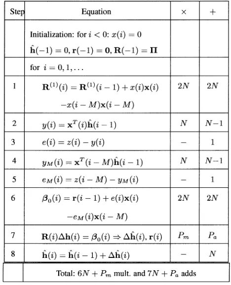
Finally, the exponentially weighted RLS algorithm is summa-rized in Table II, which also shows the complexity of different steps of the algorithm in terms of multiplications and additions. Notice that the complexity of step 5 depends on the technique used for solving the normal equation. We denote the number of multiplications and the number of additions required by the technique; these figures will be given in Section III.
B. Sliding Window RLS Algorithm
The sliding window RLS (SRLS) problem, at each sample , deals with finding a vector minimizing the error
(20)
where is the sliding window length. Solution to this problem is equivalent to solution of the normal equations (1) where the matrix and vector are updated as [2]
(21) (22)
To find the vector , we notice that
TABLE III
SLIDINGWINDOWRLS ALGORITHM
where , and
(24)
From (23) and (24), we obtain step 2 for the method in Table I:
(25)
where . Finally, the
sliding window RLS algorithm is summarized in Table III.
C. Transversal RLS Algorithms
The RLS algorithms described in Tables II and III can be used in applications with arbitrary data vectors , i.e., data vectors with no specific structure. The classical example of such applications is antenna array beamforming [1], [2].
For shift-structured input data
where is a discrete-time signal, updating the correlation matrix is significantly simplified. The lower-right
block of can be obtained by copying the
upper-left block of . The only
part of the matrix that should be directly updated is the first row and first column. Due to symmetry of the matrix, it is enough to only calculate the first column. The updating for the exponentially weighted RLS problem is described as
(26)
TABLE IV
EXPONENTIALLYWEIGHTEDTRANSVERSALRLS ALGORITHM
TABLE V
SLIDINGWINDOWTRANSVERSALRLS ALGORITHM
and, for the sliding window RLS problem
(27)
TABLE VI EXACTLINESEARCHMETHOD
III. LINESEARCHMETHODS
Many techniques can be used for solving the auxiliary normal equations (6). We are interested here in iterative algorithms as opposed to the direct solution algorithms because of lower com-putational complexity of the former. Specifically, we will con-sider line search methods that provide both a solution vector and the residual vector , which are required for applying the ap-proach described in Table I. In this section, for clarity we omit the time index from matrix and vector notations.
Solving the normal equations (6) is equivalent to minimizing the quadratic function
(28)
In a line search method, at each iteration , the solution is updated in a direction that is chosen to be non-orthogonal to the residual vector , i.e., . The step size minimizing
the function is ; this step size
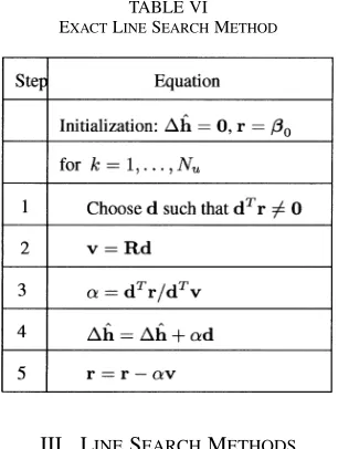
corresponds to the exact line search method [14]–[16]. A gen-eral description of the exact line search method [13] is given in Table VI, where denotes the number of iterations.
The conjugate gradient (CG) [13] and coordinate descent (CD) algorithms considered below in Sections III-A and -B, respectively, are examples of the exact line search method. Inexact line search methods, though not providing the max-imum decrement for a particular iteration, can improve the convergence speed in a sequence of iterations [15], [17]. The dichotomous coordinate descent (DCD) algorithm presented in Section III-C, is an inexact line search method.
A. Conjugate Gradient Algorithm
An efficient variant of the line search method is the CG al-gorithm [13] shown in Table VII. At the first iteration, , the direction vector is the residual vector: . At other iter-ations, , the direction is updated to guarantee -con-jugacy of the direction vectors. Due to its fast convergence, the CG method has already been used for adaptive filtering for a long time (e.g., see [5], [7], [18], [8] and references therein). Although, the CG algorithm shows fast convergence (as will be seen from simulation results in Section V), its complexity is too high for fast adaptive filtering. In general, the complexity of the
TABLE VII
CONJUGATEGRADIENTALGORITHM
algorithm is per update. The algorithm also requires di-visions at steps 1 and 3.
It can be shown that the CG adaptive algorithm as described in Tables V and VII for the particular case produces the same filter weights and output signal as the affine projection algorithm [2] of projection order and the CG adaptive algo-rithm proposed in [5].
B. Coordinate Descent (CD) Algorithm
If the directions are chosen as Euclidean coordinates, i.e., , where all elements of the vector are zeros, except the th element that is equal to one, the iterations are signifi-cantly simplified. In this case, for the exact line search,
is the th column of the correlation matrix . Thus, the most complicated step of the line search method (step 2 in Table VI), requiring the matrix-vector multiplication of com-plexity , is completely eliminated. Moreover, the other
steps are also simplified ,
and . If the directions are chosen in a cyclic order , we arrive at Gauss-Seidel iterations, and the EDS algorithm of complexity [11]. However, such choice is not efficient in our case, as it requires at least itera-tions at a time instant, resulting in high complexity. Attempts to distribute the Euclidean directions in time by assigning one direction to one time instant has led to the fast EDS algorithm [11], [9]. The maximum complexity of the fast EDS algorithm (including the filtering) is multiplications per time instant [11]. However, the convergence of the fast EDS algo-rithms is slow [11], [19]. Moreover, our simulation results (not presented here) show that the fast EDS algorithm is sensitive to the order of updating the filter weights and experiences insta-bility at the initial part of the learning process. A more efficient method for selecting the leading index is therefore important to speed up the convergence.
For the exact line search method in Table VI, we have [13]
[image:6.594.319.537.84.300.2]TABLE VIII
COORDINATEDESCENT(CD) ALGORITHM
The (nonnegative) term shows how quickly the function decreases at an update. For an exact coordi-nate search, we have
(30)
If the matrix is calculated by averaging over a relatively long time interval, are approximately constant over . There-fore, the coordinate direction chosen according to
(31)
at a particular iteration, will provide the largest decrement of . The CD algorithm with the leading index (31) is presented in Table VIII. One update in the algorithm requires only mul-tiplications and additions. Note that the CD algorithm is also known as Southwell’s relaxation method [20], [17]. Its conver-gence to the optimal solution for the normal equations follows from the following.
Theorem [17]: If the leading index of a relaxation coordi-nate descent process
for a linear system of equations with a positive-definite matrix is chosen such that, at each iteration
and if , then the process converges to the optimal solution of the system and there exists a number
, such that .
In our case, for all , we have and . There-fore, the theorem can be directly applied to the CD algorithm in Table VIII.
It can be shown that the RLS algorithm based on the CD iterations with the leading index (31) produces the same filter weights and output signal as that of the recursive adaptive matching pursuit (RAMP) algorithm proposed in [21].
TABLE IX DCD ALGORITHM
C. Dichotomous Coordinate Descent (DCD) Algorithm
The DCD algorithm [22] is presented in Table IX. It updates the solution in directions of Euclidean coordinates in the cyclic order . Such choice of directions is used in the EDS algorithm. However, in the DCD algorithm, the step-size is chosen in a different way—it takes on one of prede-fined values corresponding to binary representation of elements of with bits within an amplitude range . The algorithm starts the iterative search from the most significant bits of elements in . As the most significant bits have been updated, the algorithm starts updating the next less significant bit, and so on. Due to the quantized step-size, there are ‘un-successful’ iterations (decided at step 3) without updates of the solution and “successful” iterations where the solution and the residual vector are updated (steps 4 and 5). The DCD algorithm as described above can be found in [23].
The complexity of the DCD algorithm depends on the mentation platform. In [23], it is estimated for software imple-mentation, which usually requires an extra operation for calcu-lating at step 3. For a hardware implementation, in which we are interested here, step 3 can be considered as one addition since calculation of can be incorporated in an adder used for the comparison. The complexity can be considered as a random number with an upper bound corresponding to a worst-case sce-nario as follows. For an th bit, , within one pass there is one “successful” iteration and then, in another pass, “unsuccessful” iterations; this will re-quire additions. For the last (least significant) bit, , there are passes each with one “suc-cessful” iteration; this will require addi-tions. Thus, the worst-case complexity is
TABLE X
DCD ALGORITHMWITHLEADINGELEMENT
However, in hardware implementation one should take into ac-count the worst-case complexity.
If , the complexity of the DCD algorithm in Table IX is approximately upper bounded by . However, if the number of updates is small (which is the case that we are interested in here), the term will dominate in the DCD complexity. A computationally more efficient variant of the DCD algorithm can be proposed that eliminates this term. This new version of the DCD algorithm finds a ‘leading’ ( th) element in to be updated similarly to the CD algorithm in Table VIII. The new DCD algorithm is shown in Table X. It is seen that one update in the DCD algorithm requires bit-shifts, additions, and comparisons; the latter can be counted as additions. With updates, the complexity of the DCD algorithm is upper limited by
additions. This corresponds to a worst-case scenario when the algorithm in Table X performs all updates, i.e., the condition at step 3 is never satisfied. The important property of the DCD algorithm is that it requires no multiplication, no division, and no square root operations. Note also that the parameter defines a maximum number of filter weights that can be updated at a time instant. Thus, adaptive filtering based on coordinate descent search and, in particular, on the DCD algorithm, implements aselective partial update[24].
It is seen from the algorithm description that, in any it-eration at step 4, the step size satisfies the relationship which results in . Strictly speaking, this means that conditions of the convergence theorem in Section III-B are not satisfied at every iteration . However, as step 4 in Table X describes a quantization process, we can assume that the parameter is uniformly distributed on [1, 2) and, therefore, with probability 1, these conditions will be satisfied. Note that the decrement of the cost function (28) at every iteration is given by
(32)
which shows that the cost function decreases at every iteration.
TABLE XI
COMPLEXITY OFPROPOSED ANDKNOWNTRANSVERSAL
ADAPTIVEALGORITHMS
If, in the DCD algorithm described in Table X, step 4 is
re-placed with , we obtain
which results in . In this case, the con-vergence theorem is satisfied for . However, this choice slows down the convergence. Multiple experiments have shown that the DCD algorithm with , presented in Table X, is preferable over that with .
IV. PRACTICALISSUES
In this section, we address some practical issues related to implementation of the proposed adaptive algorithms.
For the exponentially weighted RLS algorithm in Table II, the matrix update, in the general case, requires multiplications and additions. However, if the forgetting factor is chosen as with a positive integer , then the multiplication by in step 1 can be replaced by addition and bit-shift operations, thus giving the total number of multiplications and additions and , respectively. Similar approach is also applicable to the exponentially weighted transversal RLS algorithm in Table IV, thus reducing the number of multiplications to and increasing the number of additions to . Moreover, calculation of at step 4 is also simplified to multiplications and addi-tions. However, even if is chosen differently, it is not difficult to accurately approximate it by a number making the multipli-cation by simple for implementation.
In the transversal adaptive filters, the direct copying of the matrix block would require significant pro-cessor time. To avoid the copying, a simple memory address modification can be performed, when the block does not change its position in the memory and only the row and column ad-dresses are updated. This address update was used in our FPGA design described here.
TABLE XII
FPGA RESOURCES FORERLS-DCD ALGORITHMS
ERLS-DCD algorithm requires only multiplications per sample and no division. The transversal SRLS-DCD algorithm requires multiplications and no division.
The ERLS-DCD algorithms have been implemented on a Xilinx Virtex-II Pro Development System with a XC2VP30 FPGA running at 100 MHz.1VHDL was used to describe the
design, and the Xilinx ISE 8.1 was used for synthesizing and downloading the design to the target platform.2The input data
are represented in 16-bit fixed-point Q15 format [25]. The desired signal is represented by 32 bits in the Q15 format. The matrix and vectors , and are represented by 32 bits in the Q15 format. When computing the filter output , each multiplication results in 47 bits in the Q30 format; after accumulation, is truncated to 32 bits in the Q15 format. The error signal is then represented by 32 bits in the Q15 format. The forgetting factor is chosen as , where is an integer; thus, the multiplications and are replaced by bit-shifts and additions. The FPGA resources for four designs are presented in Table XII. Two figures are shown for every resource: number of elements used and the percentage of the resource available on the FPGA device. The ERLS-DCD algorithm as described in Tables II and X was implemented for the cases and with . This design is suitable for arbitrary data vectors , e.g., it is applicable for adaptive antenna beamforming. For an 8-element antenna we obtain the update rate 205 kHz which is approximately 60 times higher than that of a design based on the QRD-RLS algorithm for 9-element antenna and with approximately the same chip area [26], [27]. The transversal ERLS-DCD algorithm with is im-plemented by using a serial design of the DCD algorithm [28] with (100 MHz) cycles for one update. The update rate can be increased by reducing and/or using a parallel design of the DCD algorithm [27]. It is seen that the whole design requires at most 10% of the resources available on the FPGA device. More details on FPGA implementation of the proposed adaptive filtering algorithms will be presented in a separate paper. We have carried out many numerical experiments with these designs, in particular, a long-time experiment where
1[Online] Available: http://www.xilinx.com 2See footnote 1.
vectors were processed. No instability problem was observed during the experiments.
V. NUMERICALRESULTS
Here, we present results obtained by computer simulation. We compare the mean squared error (MSE) performance of the proposed adaptive algorithms against the classical exponen-tially weighted RLS algorithm, NLMS algorithm, and a recently proposed efficient conjugate gradient control Liapunov func-tion (CG-CLF) algorithm with complexity [8]. Only scenarios with the time-shifted structure of input data, corre-sponding to the transversal adaptive filter, are considered. The input data are generated according to
(33)
where is the additive zero-mean Gaussian random noise with variance . The vector
contains either a real speech signal or autoregressive correlated random numbers given by
(34)
where is the autoregressive factor and are uncorrelated zero-mean random Gaussian numbers of unit variance. The MSE in a simulation trial is calculated as
(35)
The MSEs obtained in trials are averaged and plotted against the time index . Results in Figs. 1 to 5 below are obtained by floating point simulation. Fig. 6 compares floating and fixed point simulation results.
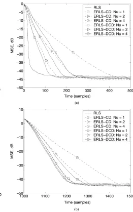
Fig. 1 shows the MSE performance of the ERLS-CG and ERLS-DCD algorithms against the RLS, NLMS, and CG-CLF algorithms. All elements of the impulse response are kept constant over the first 1000 samples; the elements are inde-pendent random numbers uniformly distributed on . At time instant , a new vector is generated and kept constant over the remaining samples. It is seen that, in the case of , the ERLS-DCD algorithm outperforms the ERLS-CG algorithm, but is inferior to the CG-CLF algorithm. For , the ERLS-DCD and CG-CLF algorithms demon-strate similar performance, whereas the ERLS-CG algorithm converges faster. For , the ERLS-DCD and ERLS-CG algorithms outperform the CG-CLF algorithm. For a fixed , the ERLS-CG algorithm converges faster than the ERLS-DCD algorithm. However, this is achieved at the expense of a sig-nificant increase in the complexity (see Table XIII). Under a fixed complexity, the ERLS-DCD algorithm provides signifi-cantly faster convergence than the ERLS-CG algorithm. Fig. 1(b) shows that after a change of the impulse response, only two updates are enough for both the ERLS-CG and ERLS-DCD algorithms to approach the RLS performance. The results for are not shown as they are not distinguishable from that of the classical RLS algorithm.
Fig. 1. MSE performance of the ERLS-CG and ERLS-DCD algorithms against the RLS, NLMS, and CG-CLF algorithms;N = 16; = 1 0 1=(2N)
0:969; = 10 ; H = 1; M = 16; = 0:9; = 0:01; N = 100. (a) Initial convergence. (b) Convergence after a change of the impulse response.
However, the performance of the ERLS-DCD algorithm is superior to that of the ERLS-CD and, as seen from Table XIII, it requires a significantly fewer number of multiplications.
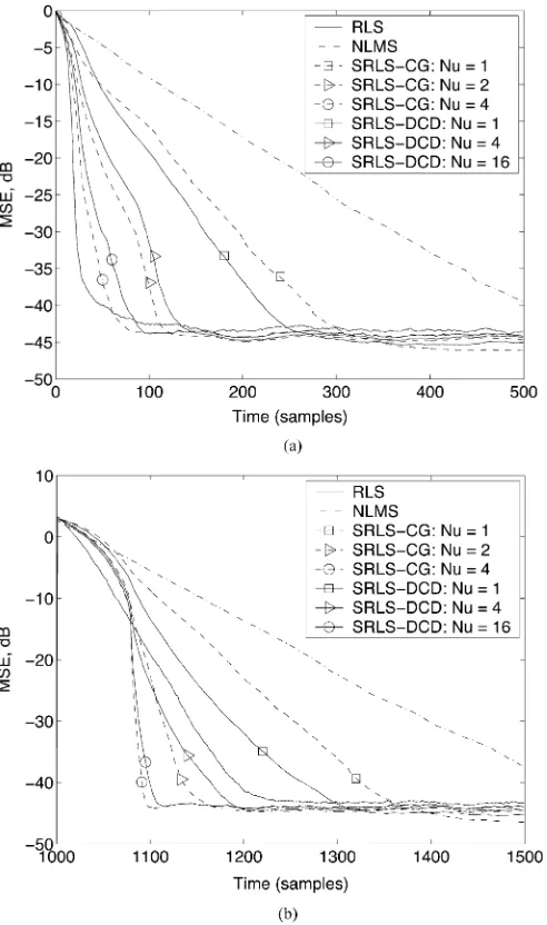
Fig. 3 shows the MSE performance of the SRLS-CG and SRLS-DCD algorithms against the RLS and NLMS algorithms. Although the SRLS-DCD algorithm has a slightly higher com-plexity than the ERLS-DCD algorithm, it achieves the same steady-state MSE more quickly, after a change of the impulse response. Therefore, for some applications, it will be benefi-cial to use the SRLS-DCD algorithm. In similarity to results for the ERLS algorithms, the SRLS-DCD requires more up-dates than the SRLS-CG algorithm to achieve the same conver-gence speed. However, the SRLS-DCD algorithm has signifi-cantly lower complexity.
[image:10.594.44.299.62.475.2]The results in Fig. 4 correspond to the application of adaptive filtering to acoustic echo cancellation with a long impulse response, . Elements of the impulse response , are independent zero-mean random
Fig. 2. MSE performance of the ERLS-CD and ERLS-DCD algorithms against the RLS and NLMS algorithms;N = 16; = 1 0 1=(2N) 0:969; =
10 ; H = 1; M = 16; = 0:9; = 0:01; N = 100. (a) Initial conver-gence. (b) Convergence after a change of the impulse response.
numbers with variance , which corresponds to a typical acoustic impulse response [29]. The vectors contain a real speech signal sampled at a frequency of 8 kHz. It is seen that with , the ERLS-DCD algorithm sig-nificantly outperforms the NLMS algorithm. With increase in , the MSE performance of the ERLS-DCD algorithm is significantly improved and, in the steady state, for , it outperforms the RLS algorithm. Table XIV shows the com-plexity of the three algorithms. It is seen that the comcom-plexity of the ERLS-DCD algorithm is significantly lower than that of the RLS algorithm and it requires only 50% more multiplications than the NLMS algorithm.
Fig. 5 shows the tracking performance of the ERLS-DCD al-gorithm in a time-varying environment. The th element of the impulse response varies in time according to
Fig. 3. MSE performance of the SRLS-CG and SRLS-DCD algorithms against the RLS and NLMS algorithms;N = 16; = 101=(2N) 0:969(for RLS),
= 10 ; M = 5N; H = 1; M = 16; = 0:9; = 0:01; N = 100. (a) Initial convergence. (b) Convergence after a change of the impulse response.
where are independent random numbers uniformly dis-tributed on are independent zero-mean Gaussian random numbers of unit variance, and is the variation rate. It is seen that as increases, the MSE performance of the ERLS-DCD algorithm is approaching that of the RLS algorithm.
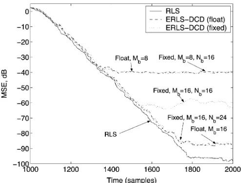
[image:11.594.42.288.65.481.2]Fig. 6 shows the performance of a fixed-point implementa-tion of the ERLS-DCD algorithm against the ERLS-DCD and classical RLS algorithms implemented in floating point. For rep-resentation of all variables in the algorithm, including the input data and , elements of the matrix and vector , etc., bits are used ( or ). It can be seen that the accuracy of both the fixed-point ERLS-DCD and floating-point ERLS-DCD algorithms depends on the parameter that de-fines the number of bits for representation of the solution vector . As increases, the steady-state MSE approaches that of the RLS algorithm. For the fixed-point ERLS-DCD algorithm, for a fixed , the steady-state MSE depends on . In this scenario,
Fig. 4. Echo cancellation experiment with a real speech signal. MSE perfor-mance of the ERLS-DCD versus RLS and NLMS algorithms:N = 512, SNR = 30 dB, = 101=(4N) 0:9995; = 0:015; H = 1; M = 16; N = 1.
Fig. 5. The tracking performance of the ERLS-DCD algorithm in a time-varying environment:F = 10 ; = 0:9; = 0:001; N = 64; =
0:975; = 10 ; N = 1.
for , the parameter limits the algorithm per-formance, while provides enough accuracy to achieve the floating-point performance.
VI. CONCLUSION
[image:11.594.306.548.313.500.2]Fig. 6. The MSE performance of a fixed-point implementation of the ERLS-DCD algorithm against the floating point ERLS-DCD and classical RLS algorithms:N = 64; = 10 ; = 1 0 1=N 0:984; = 2
10 ; N = 2; = 0; N = 1.
TABLE XIII
COMPLEXITY OFADAPTIVEALGORITHMS(N = 16)
TABLE XIV
COMPLEXITY OFADAPTIVEALGORITHMS(N = 512)
more detailed analysis of the algorithm performance will be pre-sented in another publication. A fixed-point FPGA implementa-tion of the exponentially weighted DCD-based RLS algorithms has also been described, which shows that the proposed algo-rithms are simple for finite precision implementation, require small chip resources, and exhibit numerical stability.
ACKNOWLEDGMENT
The authors would like to thank their colleague Dr. R. de Lamare for useful discussions of the techniques considered in this paper. The authors would also like to thank the reviewers for their comments.
REFERENCES
[1] S. Haykin, Adaptive Filtering, 2nd ed. Englewood Cliffs, NJ: Pren-tice-Hall, 1991.
[2] A. H. Sayed, Fundamentals of Adaptive Filtering. Hoboken, NJ: Wiley, 2003.
[3] I. D. Skidmore and I. K. Proudler, “The KaGE RLS algorithm,”IEEE Trans. Signal Process., vol. 51, no. 12, pp. 3094–3104, Dec. 2003. [4] J. H. Husoy, “Adaptive filters viewed as iterative linear equation
solvers,” inLecture Notes in Computer Science: Numerical Analysis and Its Applications. Berlin, Germany: Springer-Verlag, 2005, vol. 3401/2005, pp. 320–327.
[5] G. K. Boray and M. D. Srinath, “Conjugate gradient techniques for adaptive filtering,”IEEE Trans. Circuits Syst. I: Fundam. Theory Appl., vol. 39, no. 1, pp. 1–10, 1992.
[6] T. Bose and M. Q. Chen, “Conjugate gradient method in adaptive bilinear filtering,”IEEE Trans. Signal Process., vol. 43, no. 6, pp. 1503–1508, 1995.
[7] P. S. Chang and A. N. Willson, Jr., “Analysis of conjugate gradient algorithms for adaptive filtering,”IEEE Trans. Signal Process., vol. 48, no. 2, pp. 409–418, Feb. 2000.
[8] O. Diene and A. Bhaya, “Adaptive filtering algorithms designed using control Liapunov functions,”IEEE Signal Process. Lett., vol. 13, no. 4, pp. 224–227, 2006.
[9] T. Bose and G. F. Xu, “The Euclidean direction search algorithm in adaptive filtering,”IEICE Trans. Fundam., vol. E85-A, no. 3, pp. 532–539, Mar. 2002.
[10] G. F. Xu and T. Bose, “Analysis of the Euclidean direction set adaptive algorithm,” inProc. ICASSP’98, Seattle, WA, May 12–15, 1998, vol. 3, pp. 1689–1692.
[11] M. Q. Chen, “A direction set based algorithm for adaptive least squares problems in signal processing,” inApplied and Computational Control, Signals and Circuits: Recent Developments. Norwell, MA: Kluwer Academic, 2001, pp. 213–236.
[12] C. E. Davila, “Line search algorithms for adaptive filtering,”Trans. Signal Process., vol. 41, no. 7, pp. 2490–2494, Jul. 1993.
[13] G. H. Golub and C. F. Van Loan, Matrix Computations, 3rd ed. Bal-timore, MD: The Johns Hopkins Univ. Press, 1996.
[14] M. Al-Baali, “Descent property and global convergence of the Fletcher-Reeves method with inexact line search,”IMA J. Numer. Anal., vol. 5, pp. 121–124, 1985.
[15] Z. J. Shi and J. Shen, “Convergence of nonmonotone line search method,”J. Computat. Appl. Math. Elsevier, vol. 193, pp. 397–412, 2006.
[16] S. Boyd and L. Vandenberghe, Convex Optimization. Cambridge, U.K.: Cambridge Univ. Press, 2006.
[17] D. K. Faddeev and B. N. Faddeev, Numerical Methods of Linear Al-gebra(in Russian). St. Petersburg, Russia: Lan, 2002.
[18] M. Fukumoto, T. Kanai, H. Kubota, and S. Tsujii, “Improvement in the stability of the BCGM-OR algorithm,”Electron. Commun. Jpn., vol. 83, no. 5, pt. 3, pp. 42–52, 2000.
[19] J. H. Husoy and M. S. E. Abadi, “A comparative study of some sim-plified RLS-type algorithms,” inProc. 1st Int. Symp. Contr., Commun. Signal Process., Hammamet, Tunisia, Mar. 21–24, 2004, pp. 705–708. [20] G. Temple, “The general theory of relaxation methods applied to linear systems,”Proc. Roy. Soc. Lond. Series A, Math. Phys. Sci., vol. 169, no. 939, pp. 476–500, 1939.
[21] J. H. Husoy, “RAMP: An adaptive filter with links to matching pursuits and iterative linear equation solvers,” inProc. 2003 Int. Symp. Circuits Syst. (ISCAS’03), Bangkok, Thailand, May 25–28, 2003, vol. 4, pp. 381–384.
[23] Y. Zakharov and F. Albu, “Coordinate descent iterations in fast affine projection algorithm,”IEEE Signal Process. Lett., vol. 12, no. 5, pp. 353–356, May 2005.
[24] K. Dogançay and O. Tanrikulu, “Adaptive filtering algorithms with se-lective partial update,”IEEE Trans. Circuits Syst. II, vol. 48, no. 8, pp. 762–769, Aug. 2001.
[25] A. Bateman and I. Paterson-Stephens, The DSP Handbook: Algo-rithms, Applications and Design Techniques. Englewood Cliffs, NJ: Prentice-Hall, 2002.
[26] D. Boppana, K. Dhanoa, and J. Kempa, “FPGA based embedded pro-cessing architecture for the QRD-RLS algorithm,” inProc. 12th Annu. IEEE Symp. Field-Program. Custom Computing Mach. (FCCM’04), Napa, CA, Apr. 20–23, 2004, pp. 330–331.
[27] J. Liu, Z. Quan, and Y. Zakharov, “Parallel FPGA implementation of DCD algorithm,” inConf. DSP’2007, Cardiff, U.K., Jul. 1–4, 2007, pp. 331–334.
[28] J. Liu, B. Weaver, and G. White, “FPGA implementation of the DCD algorithm,” presented at the Commun. Symp., London, U.K., Sep. 2006.
[29] S. L. Gay and J. Benesty, Acoustic Signal Processing for Telecommu-nication. Norwell, MA: Kluwer Academic, 2001.
Yuriy V. Zakharov (M’01) received the M.Sc. and Ph.D. degrees in electrical engineering from the Moscow Power Engineering Institute, Moscow, Russia, in 1977 and 1983, respectively.
From 1977 to 1983, he was an Engineer with the Special Design Agency, Moscow Power Engineering Institute. From 1983 to 1999, he was the Head of Laboratory at the N. N. Andreev Acoustics Institute, Moscow. From 1994 to 1999, he was a DSP Group Leader with Nortel. Since 1999, he has been with the Communications Research Group, University of York, York, U.K., where he is currently a Reader. His interests include signal processing and communications.
George P. Whitereceived the M.Sc. degree in digital signal processing for communications from the Uni-versity of Lancaster, Lancaster, U.K., in 1997 and the Ph.D. degree in optimized turbo codes for wireless channels from the University of York, York, U.K., in 2001.
From 2001 to 2007, he was with the Commu-nications Research Group, University of York, as a Research Associate, publishing in fields such as coding and modulation, channel equalization for 3G, beamforming, high-altitude platform communica-tions, MIMO signal processing, and modeling of amplifier nonlinearity. He is currently a Senior DSP Engineer with the Communications Division, QinetiQ, Ltd., Worcestershire, U.K.
Jie Liureceived the B.S. degree in electronic science and technology from the Nanjing University, Nan-jing, China, in 2004.