Thesis submitted in accordance with the requirements of the University of Liverpool for the degree of Doctor in Philosophy by
Wen Yu
Abstract xi
Acknowledgements xiii
Abbreviations xv
1 Introduction 1
1.1 Overview . . . 1
1.2 Motivation . . . 4
1.3 Research Question and Related Issues . . . 5
1.4 Research Methodology . . . 6
1.5 Contributions . . . 8
1.6 Thesis Organization . . . 9
1.7 Published Work . . . 9
1.8 Summary . . . 12
2 Literature Review 13 2.1 Introduction . . . 13
2.2 Graph Mining . . . 14
2.2.1 Graph Mining Categorisation . . . 15
2.2.2 Subgraph Patterns . . . 16
2.2.3 Graph Isomorphism . . . 17
2.2.4 Canonical Forms . . . 18
2.3 Frequent Subgraph Mining . . . 21
2.3.1 The Downward Closure Property . . . 22
2.3.2 Frequency Counting . . . 22
2.3.3 The Minimum support thresholdσ . . . 24
2.3.3.1 Candidate Generation . . . 25
2.3.3.2 Frequent Subgraph Mining Algorithms . . . 26
2.4 3D Surface Representation Techniques and Grid Graphs . . . 30
2.5 Classification . . . 34
2.5.1 Semi-supervised Vertex Classification . . . 35
2.5.2 Supervised Vertex Classification . . . 35
2.5.3 Classification Techniques . . . 36
2.5.3.1 J48. . . 36
2.6.1 Accuracy, AUC, TCV and SD . . . 39
2.6.2 Overview of Statistical Performance Comparison . . . 41
2.6.3 Friedman’s Test . . . 42
2.7 Summary . . . 44
3 Application Domain and Data Sets 45 3.1 Introduction . . . 45
3.2 Application Domain One: Asymmetric Incremental Sheet Forming (AISF) and Springback Prediction . . . 46
3.2.1 AISF Process . . . 48
3.2.2 Grid Representation . . . 49
3.2.3 Springback Measurement . . . 50
3.2.4 AISF Datasets . . . 52
3.2.5 AISF Graph Translation . . . 54
3.2.6 AISF Grid Graph Statistics . . . 54
3.3 Application Domain Two: Satellite Image Interpretation . . . 55
3.3.1 Satellite Image Graph Translation . . . 60
3.3.2 Satellite Grid Graph Statistics . . . 62
3.4 Tabular format for Traditional Classification . . . 68
3.5 Summary . . . 68
4 Formalism for VULS 69 4.1 Introduction . . . 69
4.2 Formalism . . . 70
4.3 Examples of undirected VULS . . . 72
4.4 Examples of directed VULS . . . 73
4.5 Summary . . . 76
5 Algorithms for VULS Mining 77 5.1 Introduction . . . 77
5.2 The compVULSM Algorithm . . . 78
5.3 Minimal VULS Mining . . . 83
5.4 Frequent VULS Mining . . . 87
5.5 Minimal Frequent VULS Mining . . . 92
5.6 Summary . . . 95
6 Algorithm for Vertex Classification 97 6.1 Introduction . . . 97
6.2 Backward-Match-Voting algorithm . . . 98
6.3 A Working Example Using the Backward-Match-Voting Algorithm . . . . 100
6.4 Summary . . . 103
7 Experimental Results Using The Sheet Metal Forming Application 105 7.1 Introduction . . . 105
7.2 Comparison of VULS Mining Algorithms Using a Range of max Values (Objective 1) . . . 107
7.5 Comparison Between Usage of Grid Graphs and Cross Grid Graphs, and
Directed and Undirected Graphs (Objective 4) . . . 112
7.6 Effect of |LV|on Classification Effectiveness (Objective 5) . . . 113
7.7 Comparison of VULS Vertex Classification Effectiveness (Objective 6) . . 114
7.8 Statistical Comparison of the Proposed VULS Approaches (Objective 7) . 115 7.9 Summary . . . 122
8 Experimental Results Using The Satellite Image Interpretation Appli-cation 125 8.1 Introduction . . . 125
8.2 Comparison of VULS Mining Algorithms Using a Range of max values (Objective 1) . . . 127
8.3 Effect of grid size don Classification Effectiveness (Objective 2) . . . 129
8.4 Classification Effectiveness with Respect to |LE|(Objective 3) . . . 131
8.5 Comparison Between Usage of Grid Graphs and Cross Grid Graphs (Ob-jective 4) . . . 131
8.6 Effect of |LV|on Classification Effectiveness (Objective 5) . . . 134
8.7 Comparison of VULS Vertex Classification Effectiveness (Objective 6) . . 135
8.8 Statistical Comparison of the Proposed VULS Approaches on Satellite Image data (Objective 7) . . . 137
8.9 Summary . . . 140
9 Conclusion and Future Research 143 9.1 Introduction . . . 143
9.2 Summary . . . 143
9.3 Main Findings . . . 144
9.4 Future Work . . . 148
Bibliography 153 A AUC Calculation based on Mann-Whitney-Wilcoxon. 1 A.1 Introduction . . . 1
B Graph File Format and Raw Data Format 9 C Additional Experimental Results 11 C.1 Introduction . . . 11
C.2 Comparison of VULS Mining Algorithms Using a Range of max Values (Objective 1) . . . 11
C.3 Comparison Between Usage of Grid Graphs and Cross Grid Graphs, and Directed and Undirected Graphs (Objective 2) . . . 13
C.4 Effect of|LV|on Classification Effectiveness (Objective 3) . . . 14
C.5 Effect of|LE|on Classification Effectiveness (Objective 4) . . . 15
C.6 Comparison of VULS Vertex Classification Effectiveness (Objective 5) . . 16
List of Figures
1.1 Example of VULS. . . 2
1.2 Graph examples of protein networks [210] . . . 3
1.3 The VULS mining evaluation process using training and test sets . . . 7
2.1 The three main research themes of this thesis: Graph Mining, Vertex Clas-sification and 3D Surface Representation. . . 13
2.2 Venn Diagram showing the relationship between VULS, Minimal VULS, Fre-quent VULS and Minimal freFre-quent VULS . . . 15
2.3 Depth-First Search Tree and its Forward/Backward Edge Set [229]. Note that forward edges are represented by solid lines and backward edges dashed lines. . . 20
2.4 Patterns with the non-monotonic frequency [138]. . . 23
2.5 Overlapped embeddings [138]. . . 24
2.6 k-edge subgraph (k=4). . . 26
2.7 (k+1)-edge subgraphs generated by right most extension from the k-edge subgraph given in Figure 2.6. . . 26
2.8 Apriori-based (BFS). . . 27
2.9 Pattern-growth (DFS). Only frequent K-edge subgraphs will be grown to (K+ 1)-edge subgraphs. . . 27
2.10 Triangular mesh representation usingj= 3 [134]. . . 32
2.11 Rectangular mesh representation using j= 4 [134]. . . 32
2.12 Confusion matrix. . . 39
2.13 The ROC curve. The solid blue line indicates a good ROC curve that reaches the upper left corner and the dotted line indicates a random classifier (guess-ing). . . 40
44figure.caption.144 3.1 Example AISF machine 1 [129], the work piece is clamped in position while the tool head “pushes out” the desired shape; on release, springback occurs as a result of which the final shape is not the desired shape. . . 47
3.2 Example AISF machine 2, a metal sheet is clamped into a holder and the desired shape is produced using the continuous movement of a simple round-headed forming tool. . . 47
3.3 Square based pyramid (upside down) at the point when it is unclamped after application of the AISF process. . . 47
3.4 Square based pyramid (right way up); the markings are used with respect to the GOM optical measuring tool. . . 47
3.5 Example grid referenced to a central origin [129]. . . 50
3.7 Cross section at a grid line showing simple vertical springback error
calcula-tion between a before (blue line) and an after (red line) shape [129]. . . 50
3.8 Error calculation using the line-plane intersection method [129]. . . 51
3.9 Gonzalo Pyramid [184]. . . 53
3.10 Modified Pyramid [184]. . . 53
3.11 Grid representation with “Z” values (left), with corresponding grid graph where degree=4 (middle) and cross-grid graph where degree =8 (right), fea-turing “slope” labels on edges. . . 55
3.12 Example satellite image. . . 60
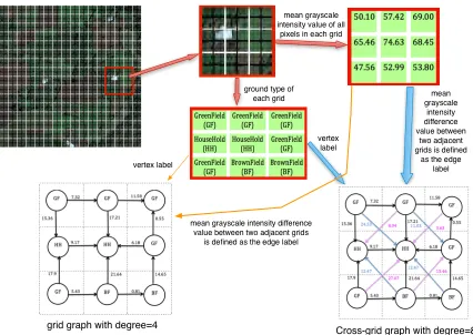
3.13 Process of Translating a satellite image into a “grid graph” and a “cross-grid graph” (the edge colour encoding is for ease of understanding only). . . 61
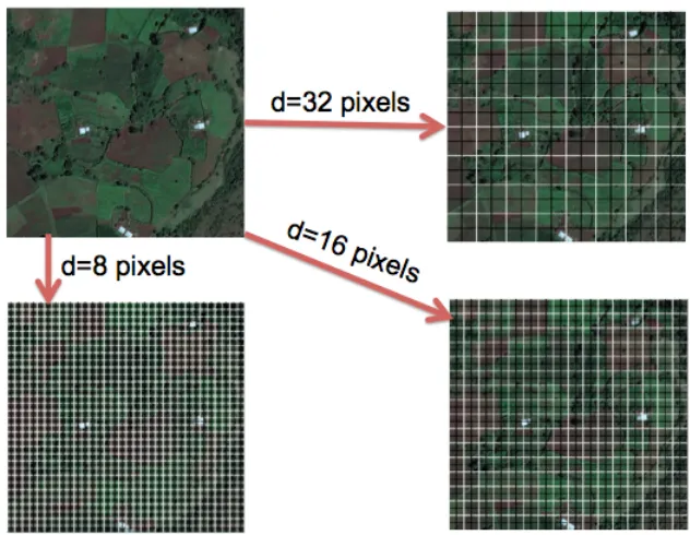
3.14 Satellite image represented in terms of three different grid squares using three different values ford. . . 62
3.15 Process for translating a grid graph into a tabular format. . . 68
4.1 Example of an undirected graph G . . . 72
4.2 One edge subgraphs contained in the example undirected graphGshown in Figure 4.1 . . . 73
4.3 Two edge subgraphs contained in the example undirected graphGshown in Figure 4.1 . . . 74
4.4 Example of directed graph G . . . 74
4.5 one edge subgraphs contained in the example directed graph G shown in Figure 4.4 . . . 74
4.6 Two edge subgraphs contained in the example directed graph G shown in Figure 4.4 . . . 75
5.1 VULS model generation process. . . 77
5.2 Example graphGtrain. . . 78
5.3 Worked example of complete VULS mining wheremax= 3 . . . 82
5.4 Input graphGtrain,G=Gtrain at the beginning of the algorithm 7 . . . 85
5.5 Example of 2-edge minimal VULSc . . . 85
5.6 G=G−c . . . 85
5.7 Example of 3-edge minimal VULS which is missed . . . 85
5.8 Worked example of minimal VULS mining where max= 3 . . . 86
5.9 Example graphGtrain. . . 88
5.10 Example of 2-edge frequent subgraphs extended from the 1-edge infrequent subgraphh B, red, Bi in Figure 5.9. . . 88
5.11 Worked example of frequent VULS mining wheremax= 3 . . . 91
5.12 Worked example of minimal frequent VULSM mining where max= 3 . . . . 94
6.1 Schematic for predicting vertex labels given a new 3D surface data set. . . . 97
6.4 Graph without vertex labels. . . 101
6.5 Four-edge pre-labelled subgraph. . . 101
6.6 Input graph G=hV, E, LEi, with unlabelled vertices, {V1, V2, . . . , V9}are vertex identifiers. . . 101
6.7 Four pre-labelled subgraphs. . . 101
6.8 Worked example of vertex classification using the pre-labelled subgraphs given in Figure 6.7 and the vertex-unlabelled graph given in Figure 6.6. . . . 102
6.9 Output graphG=hV, E, LE, LVi with predicted vertex label. . . 102
7.1 Critical difference diagram generated using Nemenyi’s post hoc test with α= 0.05 for graphs where|LV|= 2 andd= 28 (mm). . . 118
7.2 Critical difference diagram generated using Nemenyi’s post hoc test with α= 0.05 for graphs where|LV|= 3 andd= 28 (mm). . . 121
8.1 Examples of VULS identified in graphs whered= 8 pixels. . . 136
8.2 Critical difference diagram generated using Nemenyi’s post hoc test with α= 0.05 for graphs where|LV|= 2 . . . 139
8.3 Critical difference diagram generated using Nemenyi’s post hoc test with α= 0.05 for graphs where|LV|= 3 . . . 140
B.1 An example graph [122]. . . 10
B.2 GraphML encoding for the graph given in Figure B.1 . . . 10
C.1 Critical difference diagram generated using Nemenyi’s post hoc test with α= 0.05 for graphs where|LV|= 2 andd= 23 (mm). . . 21
C.2 Critical difference diagram generated using Nemenyi’s post hoc test with α= 0.05 for graphs where|LV|= 3 andd= 23 (mm). . . 22
List of Tables
2.1 DFS code for Figure 2.9 (b), (c) and (d) [229] . . . 202.2 Frequent subgraph mining algorithm categorisation [122, 140] . . . 28
3.1 Example of raw input data. . . 54
3.2 Vertex Label distribution for GS1 graph. . . 56
3.3 Vertex Label distribution for GS2 graph. . . 56
3.4 Vertex Label distribution for GT1 graph. . . 57
3.5 Vertex Label distribution for GT2 graph. . . 57
3.6 Vertex Label distribution for MS1 graph. . . 58
3.7 Vertex Label distribution for MS2 graph. . . 58
3.8 Vertex Label distribution for MT1 graph. . . 59
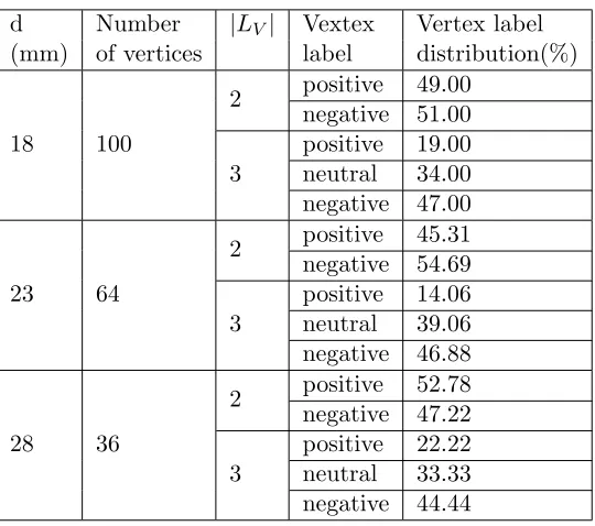
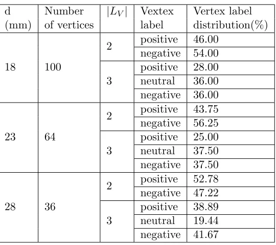
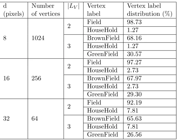
3.11 Vertex Label distribution of Satellite Image graph 2. . . 63
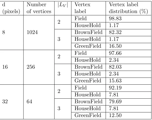
3.12 Vertex Label distribution of Satellite Image graph 3. . . 64
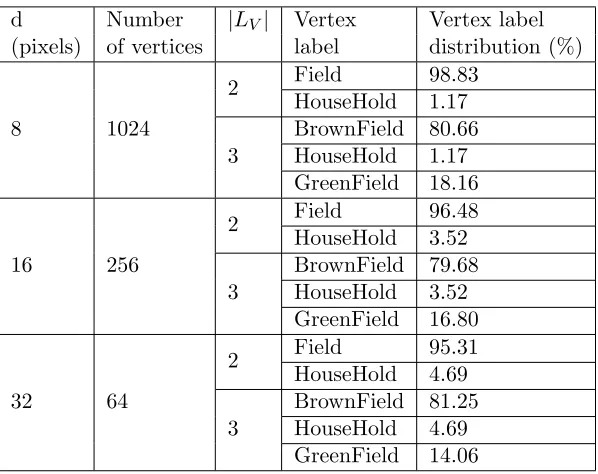
3.13 Vertex Label distribution of Satellite Image graph 4. . . 64
3.14 Vertex Label distribution of Satellite Image graph 5. . . 65
3.15 Vertex Label distribution of Satellite Image graph 6. . . 65
3.16 Vertex Label distribution of Satellite Image graph 7. . . 66
3.17 Vertex Label distribution of Satellite Image graph 8. . . 66
3.18 Vertex Label distribution of Satellite Image graph 9. . . 67
3.19 Vertex Label distribution of Satellite Image graph 10. . . 67
7.1 Evaluation Strategy Summary . . . 106
7.2 Comparison of VULS Mining Algorithms Usingmax= 4 (Objective 1). . . . 107
7.3 Comparison of VULS Mining Algorithms Usingmax= 5 (Objective 1). . . . 107
7.4 Comparison of VULS Mining Algorithms Usingmax= 6 (Objective 1). . . . 108
7.5 Classification Effectiveness with Respect tod(Objective 2). . . 110
7.6 Classification Effectiveness with Respect to|LE|(objective 3). . . 111
7.7 Classification Effectiveness with Respect to Graph Types (Objective 4). . . . 112
7.8 Classification Effectiveness with Respect to|LV|(Objective 5). . . 113
7.9 VULS Vertex Classification Comparison (Objective 6). . . 114
7.10 Average Rankings of classifiers where |LV|= 2 andd= 28 (mm) . . . 116
7.11 Average Rankings of classifiers where |LV|= 3 andd= 28 (mm) . . . 119
8.1 Evaluation Strategy Summary . . . 126
8.2 Comparison of VULS Mining Algorithms Usingmax= 4 (Objective 1). . . . 127
8.3 Comparison of VULS Mining Algorithms Usingmax= 5 (Objective 1). . . . 128
8.4 Comparison of VULS Mining Algorithms Usingmax= 6 (Objective 1). . . . 128
8.5 Classification Effectiveness with Respect tod(Objective 2). . . 130
8.6 Classification Effectiveness with Respect to|LE|(Objective 3). . . 132
8.7 Classification Effectiveness with Respect to graph types (Objective 4). . . 133
8.8 Classification Effectiveness with Respect to|LV|(Objective 5). . . 134
8.9 Classification Effectiveness with Respect to graph types (Objective 6). . . 135
8.10 Average Rankings of classifiers where |LV|= 2 . . . 138
8.11 Average Rankings of classifiers where |LV|= 3 . . . 138
A.2 Example data set . . . 2
A.1 The values (Group ID) of different combinations ofR and S based on Hand et al. [96]. . . 4
A.3 The MWW(c1|c2) value . . . 4
A.4 The MWW(c2|c1) value . . . 4
A.5 The MWW(c1|c3) value . . . 5
A.6 The MWW(c3|c1) value . . . 5
A.9 The overall AUC value for the given data set . . . 7
C.1 Comparison of VULS Mining Algorithms Usingmax= 4 (Objective 1). . . . 12
C.2 Comparison of VULS Mining Algorithms Usingmax= 5 (Objective 1). . . . 12
C.3 Comparison of VULS Mining Algorithms Usingmax= 6 (Objective 1). . . . 12
C.4 Classification Effectiveness with Respect to graph types (Objective 2). . . 14
C.5 Classification Effectiveness with Respect to|LV|(Objective 3). . . 15
C.6 Classification Effectiveness with Respect to|LE|(Objective 4). . . 16
C.7 VULS Classification Comparison where |LV|= 2 (Objective 5). . . 17
C.8 Average Rankings of classifiers where|LV|= 2 andd= 23 (mm) . . . 18
C.9 Average Rankings of the classifiers where|LV|= 3 and d= 23 (mm) . . . 19
This thesis proposes the novel concept of Vertex Unique Labelled Subgraph (VULS) mining with respect to the field of graph-based knowledge discovery (or graph mining). The objective of the research is to investigate the benefits that the concept of VULS can offer in the context of vertex classification. A VULS is a subgraph with a particular structure and edge labelling that has a unique vertex labelling associated with it within a given (set of) host graph(s). VULS can describe highly discriminative and significant local geometries each with a particular associated vertex label pattern. This knowledge can then be used to predict vertex labels in “unseen” graphs (graphs with edge labels, but without vertex labels). Thus this research is directed at identifying (mining) VULS, of various forms, that “best” serve to both capture effectively graph information, while at the same time allowing for the generation of effective vertex label predictors (classifiers). To this end, four VULS classifiers are proposed, directed at mining four different kinds of VULS: (i) complete, (ii) minimal, (iii) frequent and (iv) minimal frequent. The thesis describes and discusses each of these in detail including, in each case, the theoretical definition and algorithms with respect to VULS identification and prediction. A full evaluation of each of the VULS categories is also presented.
VULS has wide applicability in areas where the domain of interest can be represented in the form of some sort of a graph. The evaluation was primarily directed at predicting a form of deformation, known as springback, that occurs in the Asymmetric Incremen-tal Sheet Forming (AISF) manufacturing process. For the evaluation two flat-topped, square-based, pyramid shapes were used. Each pyramid had been manufactured twice using Steel and twice using Titanium.
The utilization of VULS was also explored by applying the VULS concept to the field of satellite image interpretation. Satellite data describing two villages located in a rural part of the Ethiopian hinterland were used for this purpose. In each case the ground surface was represented in a similar manner to the way that AISF sheet metal surfaces were represented, with the z dimension describing the grey scale value. The idea here was to predict vertex labels describing ground type.
As will become apparent, from the work presented in this thesis, the VULS concept is well suited to the task of 3D surface classification with respect to AISF and satellite imagery. The thesis demonstrates that the use of frequent VULS (rather than the other forms of VULS considered) produces more efficient results in the AISF sheet metal forming application domain, whilst the use of minimal VULS provided promising results
VULS based vertex classification.
This thesis would have not been completed if not for the help I have received from a number of people whose contribution to my research deserves a special mention. It is a pleasure to convey my gratitude to them all in this modest acknowledgement.
Of all the fantastic and fabulous people involved, my greatest debt of gratitude must go to my first supervisor, Professor Frans Coenen, who has given me the chance to work under his supervision. He has provided me with invaluable assistance, guidance, constant support, encouragement, constructive criticism, research ideas and excellent advice throughout the past four years, which has made it one of the most enjoyable and unforgettable experience of my life. During my PhD study, he also gave me many opportunities to publish papers and attend conferences which have helped me to broaden my horizons. I learned a lot from these conferences and workshops, these experiences remain very valuable to me. Through his extraordinary experience, he has taught me not only to be a good PhD student but also to be a good researcher and an intellectual person. He has enlightened me through his inspiration and endless efforts on how to explain and present academic work simply and clearly. He is the best supervisor any one could hope for, and more. It has been a pleasure and an honour to have been supervised by him. He was the perfect resource which inspired me and enriched my experience making me the person that I am today.
I would also like to express my great gratitude to my second supervisor, Dr. Michele Zito, who provided valuable insights and reviewed many pieces of my writings. I also thank him for providing many constructive suggestions and valuable comments concern-ing my research work.
I am also thankful to my friends and colleagues Subhieh El Salhi and Kwankamon (Kwan) Dittakan. They have been extremely helpful in providing advice on numer-ous occasions. I would like to thank Subhieh El Salhi for her valuable collaboration, especially with respect to the pre-processing of the raw sheet metal data sets used in my research. I would also like to extend great appreciation to Kwan for supplying the satellite image data sets used in the research presented here. I can not expect better friends and colleagues than Subhieh and Kwan. We encouraged each other during our PhD study. I do not believe I could have got this far without such good friends. I am also obliged to many other friends who provided encouragement, either directly or indi-rectly; they are: Maduka Attamah, Eric Schneider, Muhammad Tufail, Esra’a Shdaifat and Jeffery Raphael.
have been encouraging and helpful whenever needed. In particular, I would also like to extend my gratitude to my “PhD Advisors”: Dr. Russell Martin, Professor Paul Dunne and Dr. David Grossi for providing me with assistance, suggestions and constructive feedback at various times. I would also like to thank The Department of Computer Science at the University of Liverpool for providing me with sufficient financial assistance to attend a number of conferences/workshops and seminars throughout my study years. I am grateful for this assistance.
I would also like to extend my thanks to the Tecnalia Corporation (Spain) and the IBF institute of metal forming (Germany) for providing the before and after sheet metal forming data that I have used extensively throughout my research.
Fundamental to my being able to conduct this research was the financial support of the GuangZhou government in China, so I also would like to convey thanks to the Overseas Study Program of Guangzhou Elite Project (GEP) in China for their financial support, they have given me the opportunity to pursue my dream of studying overseas. Without their support I would have not been able to finish my research and write this thesis.
My deepest and most grateful thanks also go to my family and friends in China. Their support, trust, encouragement and thoughtfulness have been priceless to me. I am grateful to Professor Sheng Yi Jiang and Dr. Yanbo (Justin) Wang for their constant support and encouragement while in the UK, without whom the completion of my Ph.D. would not have been possible to accomplish.
Finally, I would also like to acknowledge my family and friends for all their love, motivation and support that has helped me to conduct my PhD studies. Particular thanks go to my parents A Ming Yu and Fu Ying Deng. Their love provided me with endless inspiration and was the driving force that allowed me to complete my PhD.
k-NN k-Nearest Neighbour.
VULS Vertex Unique Labelled Subgraph(s). compVULS Set of complete VULS.
minVULS Set of Minimal VULS. freqVULS Set of Frequent VULS.
minFreqVULS Set of minimal Frequent VULS. BMV Backward-Match-Voting algorithm. 3D Three Dimensional.
AUC Area Under the receiver operating Curve. SD Standard Deviation.
DM Data Mining.
FTM Frequent subTree Mining. FSM Frequent Subgraph Mining.
DCP Downward Closure Property (A graph can only be frequent if all of its subgraphs are also frequent).
DFS Depth First Search. BFS Breadth First Search. DT Decision Tree.
KDD Knowledge Discovery in Databases. RGB The Red, Green and Blue colour model. TCV Ten-fold Cross Validation.
AISF Asymmetric Incremental Sheet Forming. CAD Computer Aided Design.
CAM Computer Aided Manufacturing.
Gtrain An input training graph with vertex and edge labels. max The maximum size of labelled subgraphs such as VULS.
Gk A collection ofk-edge subgraphs.
c A candidate VULS.
S A list of potential labels for the vertices of c.
U A set of labelled subgraphs such as VULS.
|x| The cardinality of a setx.
Introduction
1.1
Overview
Data Mining (DM) is the process of extracting implicit, previously unknown, and po-tentially useful information from large amounts of data [95]. DM is an element in the Knowledge Discovery in Data (KDD) process [74, 75]. The data that data miners wish to mine comes in many different forms including: images, graphs, text and so on. There-fore the field of data mining includes sub-fields such as image mining, graph mining, and text mining. The work described in this thesis is concerned with graph mining. More specifically the work presented in this thesis proposes the concept of Vertex Unique La-belled Subgraph (VULS) mining; the identification and extraction of subgraphs (with specific configurations and edge labelings from a single graph) that have a unique vertex labelling associated with them. In other words, given a subgraphgwith a specific struc-ture and edge labelling, but no vertex labelling, and one single graph G with labelled edges and vertices. If wherever g occurs in G it always has the same vertex labelling, then g is a VULS. The utility of VULS, as will be demonstrated later in this thesis, is that they can be used to label vertices in previously “unseen” vertex unlabelled graph. A simple example is given in Figure 1.1 so as to facilitate a better understanding of the concept of VULS. With reference to input graph G in Figure 1.1, subgraph 1 is a VULS since the vertex labelling associated with the specific configuration and edge labelling in the third column is unique in the context ofG. Subgraph 2 is not a VULS since there are two possible vertex labelings (so not unique). It is important to note when considering whether a subgraph is a VULS or not that it is the vertex labelling in relation to configuration and edge labelling that needs to be unique, not the vertex labels in isolation. A VULS can include labels that appear in other VULS and other subgraphs, it is the relationship between the vertex labels that needs to be unique for a VULS to exist. The lower limit for the size of a VULS is one edge. The upper limit is the size of the input graph, in fact the entire input graph will be a VULS (although with little utility). In practice, as will become apparent later in this thesis, an upper limit is placed on the size of a VULS to ensure their utility. Further detail concerning the VULS concept are presented in Chapters 2 and 4 later in this thesis.
Figure 1.1: Example of VULS.
The essence of graph mining is the extraction of useful knowledge from graph rep-resented data. There has been a substantial amount of research effort directed at many aspects of graph mining. This research work can be loosely defined in terms of the following categorisation: (i) frequent subgraph mining [136], (ii) optimal graph pattern mining [204], (iii) correlated graph pattern mining [191], (iv) graph pattern summariza-tion [208], (v) approximate graph pattern mining [240], (vi) graph classificasummariza-tion [211], (vii) graph clustering [185], (viii) graph indexing [231, 232], (ix) graph searching [188] and (x) vertex classification [80]. The work presented in this thesis falls into the category of vertex classification. However, to the best knowledge of the author, there has been no comparable work directed at the concept of VULS mining, or the usage of VULS for vertex classification, as presented in this thesis.
Graphs are a powerful mechanism for representing structured data, for example graph vertices can correspond to objects and the edges to relationships or interactions between those objects. Two examples of the usage of graphs to represent protein networks are given in Figure 1.2 [210]. In the figures1 the vertices represent the proteins and the edges represent interactions among proteins. Generally speaking, the vertices and edges in graphs may be labelled or unlabelled. The edges may be directed or undirected. Graphs may be cyclic or acyclic. A frequently encountered type of graph structure is the Directed Acyclic Graph (DAG) structure [35, 72]. Another particular kind of graph structure, and that of specific relevance with respect to the work presented in this thesis, is the grid graph [92, 145].
Graph mining has been applied to a great variety of domains. Reported examples include: (i) chemical informatics [183], (ii) bioinformatics [54, 179], (iii) video indexing [34, 105], (iv) text retrieval [32, 162, 195], (v) Web mining, XML document mining [27, 30, 33, 38], (vi) face recognition [234] and (vii) Telecommunication and computer network analysis [19, 60, 71, 91].
1
Figure 1.2: Graph examples of protein networks [210]
The application domain at which the research presented in this thesis is directed at three Dimensional (3D) surface analysis (interpretation). 3D surface data occurs in the context of many environments. Obvious examples are applications that use map data such as geological studies [141, 154]; we might wish to predict (say) that a certain region within some given map features a particular form of geology. A less immediate example is image analysis, however images can clearly be viewed as 3D surfaces if we consider the third dimension to be “grey scale” intensity. Other applications where 3D surfaces are of significance include manufacturing processes where 3D parts are produced. One example of the latter, and that which is central to motivation for the work presented in this thesis, is sheet metal forming ([77]). The significance of 3D surface analysis, in the context of graphs is that 3D surfaces can be represented in terms of a grid, which in turn can be represented in terms of grid graph where each grid cell centre point is a vertex and each edge represents an immediate neighbourhood relationship linking adjacent grid centre points (vertices). Vertices in such grid graphs may then be labelled, for example with (say) geological labels (as suggested above) or ground surface texture labels. The central idea presented in this thesis is that given a vertex labelled grid graph, VULS mining can be applied to identify a set of VULS that can be used to predict the vertex labelling contained in previously unseen grid graphs (provided they have been drawn from the same application domain).
in Section 1.7. Finally, this chapter is concluded with a summary presented in Section 1.8.
1.2
Motivation
As noted in the previous section the focus for the work is grid graph vertex classification with application to 3D surface analysis and more particularly the sheet steel metal forming application domain. This section elaborates on the motivation for this focus.
The primary motivation for the work presented was a desire to provide a solution to an open problem in sheet metal forming whereby the produced shape is not the desired shape due to distortions introduced during the manufacturing process. In the context of the sheet metal forming motivation for the work presented in this thesis is therefore a demand for accurate and well formed sheet metal components in a variety of industries (such as the automotive and aircraft manufacturing industries). To this end there are a number of manufacturing process that can be adopted. One such process, and that used for evaluation purposes with respect to the work described in this thesis, is Asymmetric Incremental Sheet Forming (AISF). In AISF the metal sheet from which the desired component is to be manufactured is clamped into a “blankholder”, a forming tool then follows a predefined tool path to “push out” a desired shape [121]. The main advantage of AISF, over alternative sheet metal forming processes, is that of cost reduction [88, 193] (it doesn’t require heating). However, a major limitation of techniques such as AISF is that, as a result of applying the process, deformations called Springback are introduced whereby the produced shape is not the same as the desired shape. Springback is defined as the elastic deformation that occurs in a produced shape as a result of the application of a sheet metal forming process; this deformation only becomes apparent when the manufactured piece is unclamped. In other words, the produced shape differs from the desired shape. Springback is a complex physical phenomenon that is related to the local geometry of the shape to be manufactured. Essentially the shape to be manufactured can be viewed as a 3D surface which in turn can be represented in terms of a grid graph with edges representing slope (theδzvalue between adjacent grid center points). If the nature of the springback associated with individual grid graph vertices (grid cells) can be predicted then some form of mitigation can be applied; an idea first proposed in [65–67, 130]. The VULS concept proposed in this thesis therefore seems idealy suited to providing a solution to the sheet metal forming springback prediction problem. Given a manufactured part with known springback, a grid graph can be formulated with each vertex labelled with a springback value. VULS mining can then be applied and the result applied to the definition of new shapes to be manufactured.
Current work on vertex classification is directed at exploiting the topology of the graphs considered [17]. Current work is also typically not founded on graph mining techniques (as in the case of the proposed VULS technique). For example in [189, 242], a clustering approach is used, whilst in [86] a probabilistic Bayesian network model is applied and in [56] Markov random walks are used. To the best knowledge of the author the above sets the work described in this thesis apart from other existing work.
In summary the work presented in this thesis was motivated by the following:
1. A desire to address a real world problem (in the domain of sheet metal forming).
2. The need for more effective vertex classification methods directed at graph repre-sentations with a focus on grid graphs.
3. The opportunity to research an aspect of graph mining that has not previously received attention (to the best knowledge of the author).
1.3
Research Question and Related Issues
Given the motivations presented in the previous section, the main research question to be addressed by this thesis is:
“How best can the proposed VULS mining be conducted so as to achieve effective vertex classification?”
To provide an answer to this research question we also address the resolution of the following subsidiary technical research questions:
1. What is the most appropriate mechanism for identifying VULS? Al-though the fundamental idea of VULS mining seems clear, the practicalities of VULS mining, because the idea was entirely novel, remained a subject for detailed investigation.
2. Can efficiency gains be realised by mining some subset of the com-plete set of VULS?Graph mining, of all forms, is known to be computationally expensive [108, 225]; typically graph mining requires a substantial amount of iso-morphism testing [158]. Thus instead of identifying the complete set of VULS, we can attempt to identify some appropriately descriptive subset of the complete set of VULS.
4. How do we measure the quality of a set of VULS without applying them to a test set? One way of testing a set of identified VULS is to apply them in a vertex classification setting. However, in practice, this opportunity will typically not be available. An alternative VULS quality measure is thus required.
5. Once a set of VULS have been identified what is the mechanism for uitil-ising this set of VULS in the context of vertex classification? VULS are only of benefit if they can be successfully applied with respect to vertex classifica-tion, how this can best be achieved was a subject for the research.
The research presented in this thesis used sheet metal forming, particularly AISF, as a focus. There were thus also a number of subsidiary application dependent research questions that the work needed to address. Namely:
1. How best to generate the desired grid graphs from raw AISF data? In the sheet metal forming industry desired surfaces are typically specified using CAD data, while the shapes produced can be defined in terms of a point cloud obtained using some optical measuring instrument. How grid graphs can be generated from this data was unclear at the start of the research.
2. What further applications can the VULS concept be applied to? For the VULS idea to have general utility it needs to have a wide range of applicability. The nature of these further applications, applications that entail 3D surface analysis of some kind, was unclear at the commencement of the work.
The overall objective of the work presented in this thesis was thus to provide answers to the above research questions.
1.4
Research Methodology
The adopted research methodology was to commence by investigating a mechanism for identifying the complete set of VULS in a given grid graph. The start point for this work was the well known gSpan algorithm for frequent subgraph mining [229]. The gSpan algorithm operates in a Depth First Search (DFS) manner and this seemed like an appropriate strategy to be adopted for VULS mining. The gSpan algorithm also features a particular canonical form for graph representation and the concept of right most extension, both of which were adapted for the work described in this thesis.
To conduct the desired evaluation “real life” data sets, describing 3D surfaces that had been manufactured, were obtained from industry. More specifically data sets were obtained from the Tecnalia Corporation (Spain) and the IBF institute of metal forming (Germany) with whom (at time of writing) the Department of Computer Science at The University of Liverpool had contact within the context of the INnovative MAnufactur-ing (INMA) Framework 7 European project. The data sets described two flat-topped pyramid shapes referred to as the Gonzalo and Modified pyramids. In total eight data sets were obtained each comprising before and after point clouds. For further explo-ration, and to investigate the more general utility of the VULS mining concept, other forms of 3D surface were considered. More specifically satellite image data describing two villages located in a rural part of the Ethiopian hinterland were obtained using the Google Static Map Service and translated in grid graphs.
The evaluation was conducted predominantly in the context of vertex classification. The available data sets were divided into appropriate training and test sets. VULS mining was then applied to the training sets and the resulting set of VULS utilised with respect to the test sets. This process is illustrated in Figure 1.3. The resulting predicted vertex labelling could then be compared to the known labelling. The VULS mining algorithms and prediction algorithm (Backward-Match-Voting algorithm) in Figure 1.3 will be described further in Chapter 5 and Chapter 6 respectively. Standard approaches in the field of data mining, and more specifically classification, were used (such as Ten-fold Cross Validation (TCV) [79]) for testing and evaluation purposes. The metrics used to measure classification performance were accuracy, runtime, and AUC (Area Under the receiver operating Curve [9, 23, 97]). A number of additional metrics, specific to VULS mining, were also used; namely: number of VULS and coverage.
Figure 1.3: The VULS mining evaluation process using training and test sets
1.5
Contributions
The main contributions of the research presented in this thesis are:
1. The concept of VULS, which is entirely novel within the context of graph mining.
2. An alternative approach to vertex label classification that does not use a training set in the traditional form. Existing wok on vertex classification has typically adopted a traditional approach that uses a training set, comprised of a set of pre-labelled subgraphs each featuring a small number of edges and encoded in a tabular format, which is then used to generate a classifier which can then be applied to new data. This approach assumes the existence of an appropriate set of subgraphs. The proposed VULS mining automates the labelled subgraph identification process (although training data is still required).
3. Four algorithms for mining four types of VULS within a host graph. The algo-rithms can be used to find the complete set of VULS, only the minimal ones, or frequent ones, or minimal frequent ones. More specifically:
(a) compVULSMThe complete VULS mining algorithm that finds all the VULS that exist in a given input graph.
(b) minVULSM The minimal VULS mining algorithm which finds the subset of VULS whose subgraphs are not VULS (but whose supergraphs may be). The conjecture here was that this would be a more efficient form of VULS mining (than complete VULS mining) that would still realise an effective set of VULS.
(c) freqVULSMThe frequent VULS mining algorithm which finds the subset of VULS whose occurrence count is above some predefined threshold. Again the conjecture here was that this would be more efficient than complete VULS mining while still providing an effective set of VULS (in terms of vertex classification).
(d) minFreqVULSMThe minimal frequent VULS mining algorithm that finds the subset of VULS that are both minimal and frequent. The conjecture here was that minimal frequent VULS mining would combine the advantages of both minimal and frequent VULS mining.
4. The Backward-Match-Voting (BMV) algorithm for vertex classification.
5. A complete evaluation and statistical analysis of the relative merits of VULS min-ing in the context of vertex classification with respect to sheet steel formmin-ing, the primary application domain considered.
1.6
Thesis Organization
The organisation of the remainder of this thesis is as follows:
1. Chapter 2 presents the necessary background to the work described together with a review of related work.
2. Chapter 3 presents a brief description of the AISF and satellite image appli-cation domains. More specifically the datasets which were used for experimental purposes. Recall that the AISF application was used as the primary application focus for the work, while the latter was used to confirm the general applicability of the proposed VULS techniques. The necessary data preparation and image pre-processing is also described in this chapter.
3. Chapter 4 provides a formalism for the VULS concept including the four identi-fied categories of VULS: (i) complete, (ii) minimal, (iii) frequent and (iv) minimal frequent. The chapter includes simple examples of each.
4. Chapter 5 presents detail of each of the four proposed VULS mining algorithms: (i) compVULSM, (ii) minVULSM, (iii) freqVULSM and (iv) minFreqVULSM.
5. Chapter 6 describes the prediction algorithm, namely the Backward-Match-Voting (BMV) algorithm, for applying VULS in the context of vertex classification.
6. Chapter 7 gives a comprehensive experimental analysis of the nature of VULS in the context of vertex classification with respect to AISF. The chapter includes a detailed statistical analysis.
7. Chapter 8 presents an experimental analysis of the utility of VULS in the context of vertex classification with respect to an alternative application domain than sheet metal forming; specifically satellite image interpretation.
8. Chapter 9 concludes the thesis. The chapter presents a summary of the work together with the the main findings in terms of the identified research questions identified above. The chapter also presents a number of potential directions for future work founded on the research presented in this thesis.
1.7
Published Work
Some of the work described in this thesis is founded on work previously published by the author in refereed publications. These publications are itemized below, in each case the relevance with respect to the contents of this thesis is highlighted.
(a) W. Yu, F. Coenen, M. Zito, and S. El-Salhi (2015). Vertex Unique Labelled Subgraph Based Classification. Submitted for refereeing to the AI Journal. This journal paper compares the operation of earlier versions of the complete VULSM and minVULSM algorithms with respect to four different styles of grid graph: (i) degree 4 undirected, (ii) degree 8 undirected, (iii) degree 4 directed and (iv) degree 8 directed. The reported experiments indicate that the VULSM algorithm, when applied to directed grid graphs with a degree of 4, tended to produce best results. The relevance of this paper with respect to the thesis is that the paper summarised the work presented here. Note that similar experimental results to those described in the paper are presented in chapter 7.
2. Conference Papers:
(a) A. Albarrak, F.Coenen, Y.Zheng, W.Yu (2012). Volumetric Image Mining Based on Decomposition and Graph Analysis: An Appli-cation to Retinal Optical Coherence Tomography. The 13th IEEE International Symposium on Computational Intelligence and Infor-matics (CINTI2012), pp. 263-268. Budapest, Hungary. 20th-22th November, 2012. This paper considered a method for classifying volu-metric images using a decomposition and graph analysis based method. In the paper a hierarchical decomposition techniques was used to incrementally divide a given 3D volume into sub-volumes according to some critical function and then to represent the decomposition as a tree. The evaluation was con-ducted by considering the classification of 3D Optical Coherence Tomography (OCT) retinal images according to whether they feature Age-related Macu-lar Degeneration (AMD) or not (AMD is an eye condition that can result in blindness in old age). A frequent subgraph mining algorithm was applied to the tree representations and the resulting identified frequent subgraphs used to define a feature vector encoding which was then fed into a standard clas-sifier. The significance with respect to the work presented in this thesis is that the work described, although not directly concerned with vertex classi-fication, lead the author to the idea of VULS based vertex classification; the central theme of this thesis.
given input graph. The REVULSM algorithm was a preliminary version of the compVULSM algorithm presented later in this thesis in Chapter 5. The reported experimental results demonstrated that the VULS idea is sound and that the REVULSM algorithm can identify VULS in real data. The evalua-tion was conducted using the sheet steel forming applicaevalua-tion data also used in this thesis.
(c) W. Yu, F. Coenen, M. Zito, and S. El-Salhi (2013). Minimal Vertex Unique Labelled Subgraph Mining. The 15th International Con-ference on Data Warehousing and Knowledge Discovery (DaWak 2013), Springer Berlin Heidelberg, pp. 317-326. Prague, Czech Re-public. 26th-29th August, 2013. This paper built on 2(b) and proposed a minimal VULS mining algorithm, the Minimum Breadth First Search Right-most Extension Unique Subgraph Mining (Min-BFS-REUSM) algorithm, to improve the efficiency of the VULSM process (with respect to the REVULSM algorithm presented in 2(b)). The Min-BFS-REUSM algorithm was an early version of the minVULSM algorithm presented later in this thesis in Chapter 5. The reported experimental results indicated that the Min-BFS-REUSM algorithm could successfully identify all minimal VULS in reasonable time and with (in some cases) excellent coverage (an important requirement in the context of the sheet metal forming application used as a focus for the work).
(d) W. Yu, F. Coenen, M. Zito, and S. El-Salhi (2013). Vertex unique labelled subgraph mining for vertex classification. The 9th In-ternational Conference on Advanced Data Mining and Applica-tions (ADMA 2013), Springer Berlin Heidelberg, pp. 542-553. Hangzhou, China. 14th-16th December, 2013. This paper was the first to suggest that the VULS concept could be used in the context of vertex classification and proposed the Match-Voting algorithm for applying sets of identified VULS in the context of vertex classification. The Match-Voting al-gorithm was a fore-runner of the Backward-Match-Voting (BMV) alal-gorithm presented later in this thesis in Chapter 6. Experiments were conducted us-ing the REVULSM and Min-BFS-REUSM algorithms from papers 2(b) and 2(c), and the sheet metal forming application also used for evaluation pur-poses in this thesis. The results reported in this paper indicated that minimal VULS mining is both efficient and effective in term of coverage (at least in the context of the sheet metal forming application used for the evaluation).
work from 2(b), 2(c) and 2(d) by introducing the idea of frequent and mini-mal frequent VULSM. The paper included revised versions of the earlier al-gorithms for complete and minimal VULSM similar to those presented later in Chapter 5 of this thesis. This paper also presented the Backward Match Voting (BMV) algorithm for predicting (classifying) vertex labels associated with “unseen” graphs using a given collection of VULS. An extended version of the description of the BMV algorithm is presented in Chapter 6 of this the-sis. Unlike previous papers in this series the evaluation was conducted using a satellite image interpretation application (earlier papers had all used sheet metal forming as the evaluation application domain). The satellite data used describing two villages located in a rural part of the Ethiopian hinterland data. The collected satellite images were encoded in a grid format which was then converted into a 3D surface formalism by considering the average grey scale value for each grid cell as the z value. The idea here was to predict vertex labels describing ground type. A statistical analysis of the results, us-ing the Friedman test, was also presented so as to demonstrate the statistical significance of the VULS based 3D surface regional classification idea. The results indicate that the VULS concept is also suited to the task of 3D surface regional classification.
1.8
Summary
Literature Review
2.1
Introduction
This chapter presents a review of the background, related work and the application domain central to the work described in this thesis. The related work is mainly founded on three areas of research study (as shown in the Venn diagram presented in Figure 2.1): (i) Graph mining, (ii) Vertex classification and (iii) 3D surface representation. With respect to Figure 2.1 the research described in this thesis can be conceptually placed at the intersection between the three research themes. Each of the themes is considered in this chapter. We commence the discussion, in Section 2.2, with a review of graph mining techniques. One particular graph mining technique that is of significant relevance with respect to VULS mining is Frequent Subgraph Mining (FSM). This is thus considered in some detail in Section 2.3. We then go on to consider 3D surface representation and vertex classification techniques in Sections 2.4 and 2.5 respectively. A review of the evaluation metrics, and their derivation, used with respect to the work described in this thesis, is then presented in Section 2.6. Finally, this chapter is concluded with a summary in Section 2.7.
Figure 2.1: The three main research themes of this thesis: Graph Mining, Vertex
Classification and 3D Surface Representation.
2.2
Graph Mining
Graph mining is concerned with the discovery of hidden information in graph data. A graph is a set of vertices and a set of edges connecting pairs of vertices. In this thesis, and in common with much other work, graphs are also considered to have both vertex and edge labels. Thus, without loss of generality, each graph G is defined in terms of a tuple of five elements:
hV, E, LV, LE, Fi (2.1)
where:
1. V is a set of n vertices. The elements of V are denoted by the letters u or v, occasionally with subscripts if the nature of the collection of vertices is important with respect to a particular context.
2. E is a set ofmedges. The elements ofE are usually denoted by the letter e, again occasionally with subscripts.
3. LV is the set of vertex labels.
4. LE is the set of edge labels.
5. F is a labelling function that defines the mappingsV →LV andE →LE.
Each vertex (or edge) of the graph is required to have a single label; the same label can be assigned to many vertices (or edges) in the same graph. If the labelling is restricted to the vertices, or the edges, the graph is defined by a four-tuple. If no labelling is present, the graph is defined by the pair (V, E).
Throughout this thesis the expression |X| denotes the cardinality (number of ele-ments) of X, ifX is a set or an ordered sequence. However, if Gis a graph, the size of
G, is normally defined as the number of vertices or the number of edges. In this thesis
|G|=|V|(thus,|E|=O(|V|)).
If E is a collection of sets each formed by two elements of V we say that G is an undirected graph. If E is a collection of ordered pairs of elements of V then G is a directed graph. A pathP in a graphGis an ordered sequence of vertices v1, v2, . . . , v|P|
such that vi and vi+1 form an edge in G, for each i∈ {1, . . . ,|P| −1}. The graph G is
connected if every pair of vertices inG are connected by a path.
A subgraph of G is any graph φ ≡ {Vφ, Eφ, LVφ, LEφ, F} with (Vφ ⊂ V, Eφ ⊂ E, LVφ ⊂LV and LEφ ⊂LE). A candidate c of G is a subgraph of G without the vertex
labelling, thus c = {Vc, Ec, LEc, F}. Note that c may appear many times in G, there
may be a number of instances ofφ that are equivalent (isomorphic) toc.
Given a candidate c, and a graph G, a set of potential vertex labels Lv can be
byS0 the collection{Lv :v∈Vc}. A VULS ofGis a connected subgraph where|Lv|= 1
for each Lv ∈S0.
Referring back to the introduction to this chapter, other than “standard” VULS as defined above, we can identify three other kinds of VULS: Minimal VULS, Frequent VULS and Minimal frequent VULS.
Definition 1: Minimal VULS. A minimal VULS is a VULS such that none of its subgraphs are VULS.
Definition 2: Frequent VULS.A Frequent VULS (FVULS) is a VULSφ
whose occurrence count,Occurrence(φ), within the input graphG, is greater than some pre-specified thresholdσ.
Definition 3: Minimal frequent VULS.A minimal frequent VULS is a VULSφwhich is both minimal and frequent.
The relationship between the different forms of VULS is illustrated in Figure 2.2. The relevance of the numbering included in Figure 2.2 will become clear later in chapter 4. The concept of VULS will be considered in further detail, with some worked examples, in chapter 4.
Figure 2.2: Venn Diagram showing the relationship between VULS, Minimal VULS,
Frequent VULS and Minimal frequent VULS
This section is organised as follows. Section 2.2.1 presents an overview of the research domain of graph mining starting with a categorisation of this domain. Graph mining often involves the identification of patterns (subgraphs or subtrees) in graph data. There are various forms of graph pattern that may be of interest and these are reviewed in section 2.2.2. Subgraph isomorphism is a central activity frequently required for graph mining and this is discussed in section 2.2.3. Another important aspect of graph mining is the mechanisms whereby graphs are represented so as to facilitate mining; some kind of canonical form is required, and this is therefore discussed in section 2.2.4.
2.2.1 Graph Mining Categorisation
single graph mining. In transaction graph mining [47, 115, 118, 136, 221] the input comprises a collection of graphs and the objective is to find hidden patterns that exist across this collection. Transaction graph mining is essentially an extension of frequent items set mining [2, 21, 93, 94] as used with respect to tabular data. In single graph mining the input comprises a single large graph and the objective is to find patterns that exist within this single large graph. An application domain where single graph mining is often applied is social network analysis [3, 133, 203]. Examples of social networks include twitter communities, Facebook communities, and co-authoring networks. The work presented in this thesis belongs to the single graph mining category.
Alternatively, graph mining when used for classification purpose can be divided into two categories: (i) graph classification and (ii) vertex classification. With respect to the first category the objective is to use pre-labelled training graphs to produce a classifier with which to classify previously unseen graphs [128]. From the literature we can identify a number of graph classification approaches, these include: LEAP [230], gPLS [182], CORK [205], and COM [123]. With respect to the second category the objective is to train a classifier, using training data, so as to construct a classifier that can be used to classify (label) vertices whose labels were previously unknown. Vertex classification may be conducted within a single graph (where some of the vertices have been pre-labelled for training purposes) or across a collection of graphs (where the vertices in some graphs have been pre-labelled for training purposes). The work presented in this thesis is particularly concerned with the concept of vertex classification and thus the principles of vertex classification are considered in further detail in Section 2.4 later in this chapter.
2.2.2 Subgraph Patterns
As will become apparent later in this thesis, the proposed VULS mining methods used in this work, especially frequent VULS and minimal frequent VULS mining, “borrow” concepts and techniques from the domain of FSM (Frequent Subgraph Mining), thus VULS mining techniques also fall into the second of the above categories. From the literature the most common types of frequent subgraph that can be mined include: (i) “ordinary” frequent subgraphs [109], (ii) closed frequent subgraphs [39, 43, 228], (iii) maximal frequent subgraphs [106, 207], (iv) approximately frequent substructures [240], (v) contrast substructure [46], and (vi) discriminative frequent substructures [124, 232]. The first of the above, ordinary frequent subgraphs, is the most relevant to VULS mining, especially frequent VULS and minimal frequent VULS mining. Because of its significance with respect to the work presented in this thesis frequent subgraph mining is discussed in further detail in Section 2.3 later in this chapter.
2.2.3 Graph Isomorphism
Graph isomorphism is concerned with the problem of deciding whether two graphs are identical or not. In other words, given two graphs, does there exist a one to one mapping of the vertices in one graph to the vertices in the other such that vertex adjacency is preserved [78]. Isomorphism testing is computationally expensive. This is particularly the case with respect to frequent subgraph mining (see below) because of the large num-ber of graph comparisons that need to be made; graph isomorphism plays an essential role in determining whether a candidate subgraph exists within a given graph and how often it exists. Isomorphism testing also plays a significant role with respect to vertex classification (see section 2.5 below). Subgraph isomorphism with respect to non-regular graphs is known to be a NP-complete1 problem [78], no algorithm has been found that can solve the isomorphism testing problem in polynomial time [49, 85]. However, sub-graph isomorphism with respect to trees, permutation sub-graphs, chordal sub-graphs and grid graphs (as used in this thesis) is not a NP-complete problem [78]. Note that a tree is a graph containing no cycles [216], and a grid graph is a node-induced finite subgraph of the infinite grid [119].
There has been much work on algorithms to enhance the efficiency of isomorphism testing; examples include: (i) Ullmann’s algorithm [160, 215], (ii) Backtracking algo-rithm [186], (iii) Nauty [157], (iv) VF and VF2 using a State Space Representation (SSR) [48, 49] and (v) geometric isomorphism [139]. However, none of these existing isomorphism detection algorithms are entirely suited to VULS mining, or VULS based vertex classification, as envisioned in this thesis. The reasons for this are:
1. Most existing isomorphism approaches use vertex invariants (such as the degree of a vertex, the “twopaths” concept, adjacency triangles, k-cliques, independent k-sets and distances) to solve the isomorphism problem [78]. However, calculation
1
of the invariant values, especially with respect to the more complex invariants, is time consuming; it is also very difficult to determine which invariant is the best for a particular graph. Instead, what is typically done is to leave the decision of if and when to use a vertex invariant up to the user (except for degree which is always used). Given a number of complex graphs, time would be required to experimentally determine what invariant to use.
2. Most of above isomorphism approaches use adjacency matrixes to represent graphs, which is not well suited in the context of the VULS mining proposed in this thesis.
Thus the isomorphism testing approach used with respect to the work presented in this thesis is based on that espoused within the gSpan frequent subgraph mining algorithm [229]. The gSpan isomorphism approach is to take a single graph G and apply some function C(G) which returns a canonical label such that C(G) = C(H) iff G and H are isomorphic. In other words, gSpan addresses the graph isomorphism problem by comparing the “canonical labellings” of two graphs. If these labellings are the same, then these graphs are isomorphic. The concept of canonical labelling (forms) is described in more detail in the next section. The gSpan algorithm is considered in further detail in Section 2.3 later in this chapter.
2.2.4 Canonical Forms
A canonical form is an agreed way of representing some object (such as a graph). In the context of graph mining canonical forms are important so that the relevant algorithms can be both effective and efficient [177, 222]. In the case of isomorphism testing canonical forms are significant so as to ensure that, given two identical graphs, they are represented in the same manner (thus simplifying the isomorphism testing). In other words, a canonical form facilitates isomorphism checking because it ensures that if a pair of graphs are isomorphic, then their canonical labellings will be identical [20, 117, 136, 177]. In the case of graph mining algorithms that involve the generation of candidate graphs, such as the VULS mining algorithms with respect to this thesis, the usage of a canonical form is important so as to avoid the generation of duplicates (the same graph but expressed in different ways).
described in this thesis, Minimum DFS Coding, was adopted because of its popularity in the context of frequent subgraph mining.
Depth-First Search (DFS) is an algorithm for traversing or searching tree or graph data structures. One starts at the root (some arbitrary vertex in the case of a graph) and explores each branch before backtracking. This requires some ordering of vertex identifiers; given two branches emanating from a vertex some ordering needs to be imposed so that one branch is selected before the other. In the case of graphs a similar mechanism needs to be imposed to select a start vertex.
For one graphG, there are lots of ways to construct different DFS trees by selecting a different rootU and different growing edges. When performing a depth-first search in a graph, various DFS trees can be constructed each with its own DFS code. In other words, a lot of DFS codes can be adopted to represent a graphG, to prevent ambiguity we require a canonical form so that among all these DFS codes, there is only one minimal DFS code. It is this minimal DFS code that will then be employed to represent G. In the following, how to generate various DFS codes for graph G is described first. Then an example is given to illustrate such process and how to choose the minimal one as the canonical form from the various DFS codes generated is also explained at the same time.
The DFS code for a graph consists of a sequence of tuples describing the edges in a given graphG. The tuples are of the form:
hU, V, LU, LE, LVi
where: (i) U is the identifier for the start vertex, (ii) V is the identifier for the end vertex, (iii) LU is the vertex label for U, (iv) LE is the edge label and (v) LV is the
vertex label forV. The DFS codes for Gis generated as follows:
1. Impose an ordering on the vertices (a sequential set of unique vertex identifiers). Mark all edges as “unread”.
2. Select the first vertex in the ordering as the root (the start point) U.
3. Create an ordered list of edges{e1, e2, . . . , en}emanating from rootU. List
back-ward edges prior to forback-ward edges.
4. Process the edge list {e1, e2, . . . , en},i= 1 (16i6n):
(a) Ifeiis marked as being “unread”, create a code describing the edge and store,
mark the edge as “read” and proceed to (b).
(b) Ifei is a forward edge, choose the end vertex of ei as rootU, repeat from 3.
Figure 2.3: Depth-First Search Tree and its Forward/Backward Edge Set [229]. Note
that forward edges are represented by solid lines and backward edges dashed lines.
Table 2.1: DFS code for Figure 2.9 (b), (c) and (d) [229]
edge NO. (b) (c) (d)
0 h0,1, X, a, Yi h0,1, Y, a, Xi h0,1, X, a, Xi
1 h1,2, Y, b, Xi h1,2, X, a, Xi h1,2, X, a, Yi
2 h2,0, X, a, Xi h2,0, X, b, Yi h2,0, Y, b, Xi
3 h2,3, X, c, Zi h2,3, X, c, Zi h2,3, Y, b, Zi
4 h3,1, Z, b, Yi h3,0, Z, b, Yi h3,0, Z, b, Xi
5 h1,4, Y, d, Zi h0,4, Y, d, Zi h2,4, Y, d, Zi
For instance consider the graph G given in Figure 2.3 (a). From this graph various DFS trees can be generated depending on the choices of the rootU among the vertices. Figure 2.3(b), (c) and (d) give three different DFS trees for the graph in Figure 2.3(a). If we choose the first “X” in Figure 2.3(a) as the rootU, the DFS tree shown in Figure 2.3(b) will be generated. In the same manner, if we choose “Y” or the second “X” as the root. The trees shown in Figures 2.3(c) and (d) would be generated. Thus G can be represented as three different ways. Therefore there are three different DFS codes one per DFS tree as shown in Table 2.1 to represent the same graphG(Figure 2.3(a)). Note that forward edges are represented by solid lines and backward edges dashed lines. The question is how to find the minimal DFS codes from these three DFS codes.
The minimum DFS code, as the name suggests, is the minimum code according to some lexicographic order of the graph edges. In other words, an ordering is imposed on the element values with respect to five tuples hU, V, LU, LE, LVi. Thus, in Table 2.1,
two elements are the same (1 and 2), the third element “X” is before “Y”, thus DFS code (d) is smaller than (b). Thus, (d) is the minimum DFS code for G and thus it is the unique canonical form with which to represent G (Figure 2.3(a)). Note that a subgraph is a duplicate subgraph if and only if its DFS code is not minimum.
Given two graphs G and G0, G is isomorphic to G0 if and only if the minimum DFS code of G is identical to the minimum DFS code of G0. The isomorphism testing process is given in algorithm 1. If the minimum DFS codes of two graphs are not the same, the two graphs are not identical. Thus the problem of mining subgraphs can be said to be equivalent to analysing their corresponding minimum DFS codes. Note that the minimal DFS code is dependent upon the global set of labels in an input graph or set of input graphs. Thus any two subgraphs that subscribe to this global labelling can still be compared; of course if they do not subscribe to this global labelling then comparison is not possible. As will become apparent later in section 2.3.3.2, the use of minimum DFS codes can enhance the process of frequent subgraph mining by comparing the minimal DFS code of two graphs to do the isomorphism testing. Thus for the VULS classification proposed in this thesis, minimum DFS coding was adopted for subgraph matching (subgraph isomorphism) with respect to both the VULS mining and vertex classification by VULS.
Algorithm 1
1: procedure IsomorphismTest(G,G0)
2: S= the set of minimal DFS codes for graph G 3: S0= the set of minimal DFS codes for graphG0 4: result=true
5: if |S|!= |S0|then
6: result=false
7: else
8: forall i from 1 to|S|do
9: if Si6=Si0 then
10: result=false
11: return result
12: end if
13: end for
14: end if
15: return result
16: end procedure
2.3
Frequent Subgraph Mining
presented in this thesis “borrows” ideas from the concept of FSM and especially the well known gSpan algorithm [229]. More specifically: (i) some general ideas concerning FSM were incorporated into the proposed VULS mining; and (ii) frequent VULS mining and minimal frequent VULS mining, a variation of the proposed generic VULS mining, was founded on the idea of FSM. FSM algorithms, typically operate using a candidate gen-eration, frequency counting and pruning loop; the proposed VULS mining algorithms operate in a similar manner although (except in the case of frequent VULS or minimal frequent VULS mining) without the frequency counting element.
There are a great variety of FSM algorithms. Some of which were developed for transaction graph mining and have subsequently been used for single graph mining and others that have been specifically designed for single graph mining. It should also be noted that many subgraph mining algorithms are extensions of subtree mining algo-rithms which in turn are often extensions of frequent item set mining algoalgo-rithms as used with respect to binary valued tabular data [11, 122]. Recall also that a tree is a special form of graph that offers advantage in the context of graph mining, namely that can-didate generation and isomorphism testing is much more straight forward than in the case of graphs.
In the context of FSM, particularly when applied to transaction graph data, a concept known as the Downward Closure Property (DCP) or the anti-monotone property of itemsets is often utilised. This is an important concept with respect to both FSM and frequent VULS mining, thus is discussed in further detail in Section 2.3.1 below. A central element of FSM algorithms is the mechanism used to determine the frequency of subgraphs, this is thus discussed in Section 2.3.2. To determine whether a subgraph is frequent or not its occurrence count is typically compared with a frequency thresholdσ, the nature of this threshold is discussed in Section 2.3.3. Candidate generation is then considered in Section 2.3.3.1.
2.3.1 The Downward Closure Property
In the context of transaction FSM, where frequency is counted in terms of one count per transaction in which some subgraphg appears, the downward closure or anti-monotone property states that if g is not frequent none of its supergraphs can be frequent. This is significant with respect to FSM candidate generation as discussed in the following subsection. In some cases the Downward Closure Property (DCP) may apply in the context of single graph mining depending on how the frequency counting is conducted [187, 197, 218]. However, in the context of VULS mining, as will be demonstrated in Chapters 4 and 5, this does not apply; ifg is not a VULS this doesnotmean that none of the supergraphs ofg are also not VULS.
2.3.2 Frequency Counting
Figure 2.4: Patterns with the non-monotonic frequency [138].
support2 is used to describe the occurrence or frequency count of a graph. There are a variety of ways that support can be defined. In part this is dependent on the nature of the FSM problem: transaction graph based or single graph based. In transaction graph mining the options are whether: (i) to consider the presence of a particular subgraph
g in a transaction graph t to represent a count of one regardless of how many timesg
actually occurs in t, or (ii) to take into account the occurrences of g in t. We refer to the second as occurrence counting. In single graph mining the only option is to adopt occurrence counting and take into account occurrences ofg. Given that the focus of this thesis is on single graph mining the discussion on support counting presented in this section is directed solely at mechanisms in the context of single large graphs [26, 76].
In general, in the context of single graph mining, there are two possible methods for determining the frequency of a subgraph. In the first, two embeddings of a subgraph are considered different, as long as they differ by at least one edge (non-identical). As a result, arbitrary overlaps of embeddings of the same subgraph are allowed. In the second, two embeddings are considered different, only if they are edge-disjoint. These two methods are illustrated in Figures 2.5 and 2.4. In the example presented in Figure 2.5 there are three possible embeddings of the subgraph shown in Figure 2.5(a) in the input graph given in Figure 2.5(b). Two of these embeddings (shown in Figures 2.5(c) and (e)) do not share any edges, whereas the second embedding (Figure 2.5(d)) shares edges with the other two. Thus, if we allow overlaps, the frequency of the subgraph is 3, and if we do not it is 2.
2Support can be defined in general as the proportion of occurrence of a subgraph over a total number