Hall coefficient and resistivity of an amorphous palladium silicon alloy

HALL COEFFICIENT AND RESISTIVITY OF AN AMORPHOUS PALLADIUM-SILICON ALLOY

Thesis by Raymond Dean Ayers

In Partial Fulfillment of the Requirements for the Degree of

Doctor of Philosophy

California Institute of Technology Pasadena, California

1971

i i i •

ACKNOWLEDGMENT

I would like to thank Dr. R. H. Willens for suggesting the experimental problem and the National Aeronautics and Space

ABSTRACT

The Hall coefficient and resistance in several specimens of an amorphous metallic alloy containing 80 at.% palladium and 20 at.% silicon have been investigated at temperatures between ~.2°K and room temperature. An ideal limiting behavior of these transport

coefficients was analyzed on the basis of the nearly free electron model to yield a carrier density of 9 x 1022 cm.-3 , or about 1.7

0

electrons per palladium atom, and a mean free path of about 9A which is almost constant with temperature. The deviations of the individual specimens from this ideal behavior, which were small but noticeable

v.

TABLE OF CONTENTS

I. INTRODUCTION

I I. EXPERIMENTAL PROCEDURE

A. Preparation and testing of Hall effect specimens 2 B. Resistivity and Hall coefficient measurements 3

C. Additional resistivity measurements 8

D. Preparation of annealed and equilibrium specimens 8

I I I. EXPERIMENTAL RESULTS IV. DISCUSSION

V. HALL COEFFICIENT IN A TWO-PHASE SYSTEM

A. Current density in an isolated crysta 1 B. Effects of many crystals

c.

The Ha 11 voltage

D. The geometrical amplification factor

E. The Ha 11 coefficient of the connected F. Magnetoresistance

G. Application to the present results

References

phase

9

li.J

18 27 3Lj 38 '-l3 Ljs Lj7

After the accidental discovery that gold-sil icon alloys could ( 1 ) be retained in a non-crystalline solid phase by rapid quenching

the first of several other such amorphous phases to be found by a

systematic search was in the neighborhood of the very deep eutectic ( 2 )

at 15.5 at.% Si in the system Pd-Si. Because of the relative

ease with which a successful quench could be obtained, the particular

composition Pd

₈

Si was singled out for intensive investigation by

• • 2 ( 3 )

X-ray diffraction, electron microscopy and resistivity measurements.

The results of that work tended to confirm the belief that this

really was a metallic system with only very short range order. The

present investigation of the Hall coefficient in the same alloy was

undertaken to see whether this transport coefficient could be

interpreted in terms of the nearly free electron model (spherical

Fermi surface, effective mass very near to the true mass of the

electron) that has proved so useful in understanding electrical

2 I I. EXPERIMENTAL PROCEDURE

A. Preparation and testing of Hall effect specimens

The alloy containing 20 atomic percent silicon and 80 atomic

percent palladium was prepared by radio frequency induction melting

in a fused silica crucible under an argon atmosphere. The palladium

metal, obtained from Engelhardt Industries Inc., was 99.~/o pure with an

iron content of about 100 parts per million, and the silicon was

transistor grade. Small samples of the alloy were rapid-quenched ( ~ ) from the molten state by the "pis ton and anv i 111 _technique

producing foils about 3 em. in diameter and 40 to 50 microns thick.

Each foil was examined by means of X-ray diffraction to determine

whether any misquench crystals were present. This was done in

0 reflection on a Norelco goniometer using a scanning speed of 0.1 /min.

and CuK~ radiation. The range of angles covered (29 • 36° to 44°)

included the first broad amorphous band, and any foils that showed

either a narrowing of the band or sharp peaks superimposed on the

amorphous pattern were rejected ~bout 6~/o of those tested).

The remaining foils that were large enough to provide a Hall specimen

were cut into rectangular strips about 1 em. wide and four platinum

leads were spot-welded along the length of each strip. By means of a

potentiometric measurement the temperature coefficient of resistance

was detennined crudely by comparison of the values at the boiling

highest residual resistivity, and hence the lowest fractional

temperature coefficient of

resistancejt~~

were chosen for preparation as Hall effect specimens. In addition, representative foils with

lower residual resistivities were also selected. Each of the foils selected for Hall specimen preparation was clamped between two 1/411

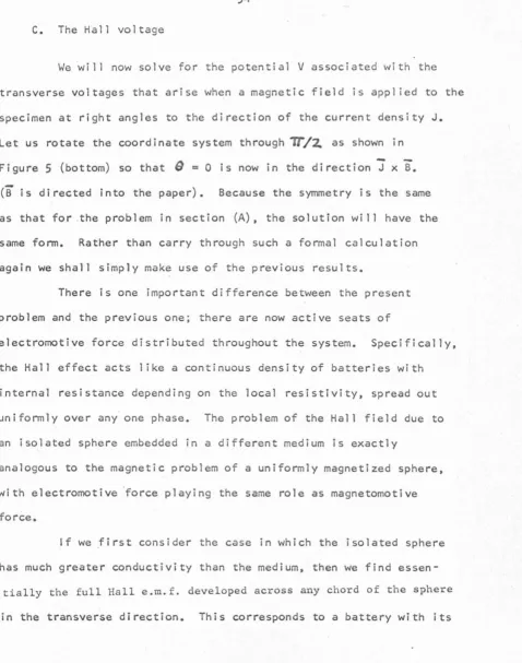
thick pieces of brass and milled to the dimensions shown in Figure 1.

The 11_ears11 _{labelled A and B were used to provide the current to the}

specimens; the Hall voltage was measured between C and D, and the voltage drop between E and F was used to determine the temperature dependence of resistance. A final check for misquench crystals was made on each specimen by taking four or five X-ray exposures in

transmission Laue geometry with Mo~ radiation to examine the region between the Hall ears. In none of the exposures was there any indi-cation of granularity to the broad amorphous bands or sharp spots superimposed on them. For the first few specimens, fine platinum wires were spot-welded to each of the ears, but it was found that this method produced an electrically noisy contact probably due to the presence of an A.C. rectifying oxide layer. In later work the contacts were made by soldering fine copper wires to the ears with

indium metal.

B. Resistivity and Hall coefficient measurements

The Hall specimen was then connected into the circuit shown

in Figure 2. A current of about 200 rnA. was provided through the

A

.0

4

11

E

_j_

I

T

c

D

I

I

T

_.875"

.026

II

.43

75

II

F

I

j_

8

~.1875'~

Figure 1. Dimensions of the Hall effect specimen~.

[image:9.564.97.457.57.677.2]

(11Air cells11) in series with a lO.Jl. resistor and a shunt box for

measuring the current with a Leeds and Northrup guarded potentiometer.

6

During the measurements this current was stable to one part in 10 •

The guarded potentiometer was also used to measure the voltage drop

across the ears E and F in determining the resistance and the voltage

developed in a copper-constantan thermocouple circuit with one junction

near the specimen and the other in a reference ice bath.

The Hall voltage developed across ears C and 0 was measured

with a Leads and Northrup Wenner potentiometer. The galvanometer

output from the Wenner was fed into a Keithley nanovoltmeter where it was amplified and sent on to an A.Z.A.R. recorder. Most of the

-4

voltage (on the order of 10 volts) across these ears was simply the iR

drop due to the fact that the leads could not be located exactly opposite each other. The Hall voltage was much smaller than this (on

the order of 10-l volts), so a measurement was performed by

reversing the magnetic field and taking half the difference of the

voltages for the two field directions as the Hall voltage.

The magnetic field normal to J and EH was provided by a 12

inch Varian electromagnet with a 2.75 inch pole gap. The magnetic field was measured with a Varian F-8 nuclear magnetic resonance

fluxmeter.

In order to reduce noise due to thermoelectric voltages in

the Hall circuit and to remove the possibility of a systematic error

arising from the Ettinghausen effect, it was found necessary to

KEITHLEY

I

A.Z.A.R.

NANOVOLTMETER

RECORDE

D

La

N

WENNER

POTENTIOMETER

MAGNETIC

FIELD

T.C.

L

a

N

GUARDED

POTENTIOMETER

REFERENCE

BATH

Figure

2.

Circuit

for

measuring

Ha11

coefficient

and

resistance.

coefficient was measured only at room temperature and the boiling points of liquid He, N and Freon 22. All measurements were made with the

2

specimen in a liquid helium glass Dewar; for the Freon 22 measurements

the specimen was immersed in alcohol and the jacket between the

liquid He and liquid N containers was filled with He gas to transfer 2

heat to the Freon in the outer Dewar.

At any one temperature the Hall voltage was measured for both directions of current and several values of the magnetic field, in addition to the reversal of field directions already mentioned. The Hall coefficient was found to be independent of field strength and there was no change on reversing the current. The specimens were also tested for transverse magnetoresistance by comparing the potential drop across ears E and F with no magnetic field and with

8

k G. To within

8

the limits of sensitivity of the potentiometer (one part in 10) there was no difference.

After the electrical measurements were completed, the thick-ness of the foils in the region between the Hall ears was determined by taking the average of several readings with a micrometer caliper having a large jaw and a fine one. Attempts to corroborate these

measurements with·X-ray absorption showed that the foils contained

many fine holes. The percent error introduced in the absolute values of the Hall coefficient and resistivity by the thickness measurement was much greater than that due to any other parameter. Fortunately

8

c.

Additional resistivity measurements

Resistivity values at temperatures between those of the

isothermal baths were obtained using the apparatus described in

reference ( 5 ). The specimens were mounted four at a time inside

a brass chamber contained in a 1 iquid helium double dewar.

Quasi-0

isothermal measurements were performed at an interval of about 3 K

as the temperature of the chamber gradually rose. About 8 hours were

allowed for the range from 4.2°K to 77°K, and the warming from 77°K

to room temperature took about 30 hours with an intermittent flow of

He gas regulating the rate of temperature rise.

D. Preparation of annealed and equilibrium specimens

In addition to the as-quenched specimens described in part A,

a specimen showing no initial crysallinity was sealed under vacuum

in a fused silica tube and annealed for 12,000 hours at 225°C. The

foil was then re-examined by X-ray diffraction and found to have a

small, sharp peak superimposed on the first broad amorphous band.

Another specimen was annealed to the equilibrium phases

(Pd

3Si, perhaps Pd9si2 and others) by maintaining it under vacuum at 750°C for one week. Both foils were prepared as Hall specimens

and subjected to the measurements described in part B. Because of

its brittleness the equilibrium specimen was not mechanically

machined to give the correct Hall geometry, but instead electrical

I I I. EXPERIMENTAL RESULTS

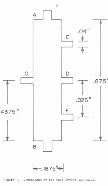
The resistance of each specimen, expressed as a ratio to its

room temperature value, Is plotted as a function of temperature in Figure

3.

The individual data points have not been reproduced because

they are too closely spaced. The possible error involved in each

measurement Is about ~ 0.5°K and~ 0.1% relative resistance. The

values obtained from the isothermal measurements agreed with these

curves to within the specified accuracy. Specimen No. 1~0 was

broken before it could be subjected to the quasi-isothermal

measure-ments; Its resistivity ratio at 1 iquid He

2 temperature was 0.969. At the same temperature the resistivity ratio for the 12,000-hour

anneal specimen was 0.951 and that for the equilibrium specimen was

0. 172.

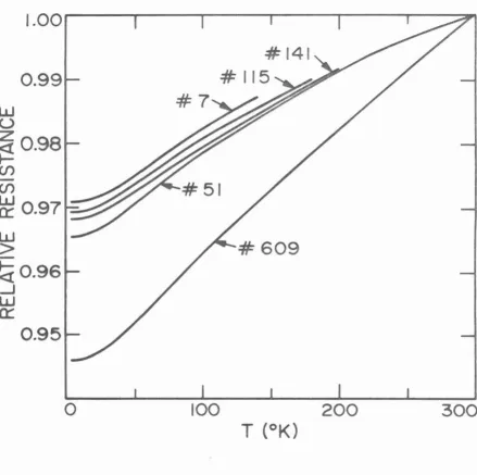
The negative absolute Hall coefficient of each specimen is

plotted as a function of temperature in Figure~. The statistical

scatter in repeated measurements of a single data point corresponded -11 3

to about + 0.1 x 10 m /coulomb, or about + ~lo of the largest values obtained, but there is likely to be a much greater error In the determination of the thickness of each specimen, which enters

as a multiplicative factor for each curve. The size of that error

might be as much as~ 1~/o, with the error much more likely to be on

w

u

1.00

0.99

ao.9a

_{.,._.:}

(f) (f)

~0.97~

w

>

~0.96

_J

w

Cl::

0.95

0

10

#141

#115

100

200

300

[image:15.558.47.486.168.605.2]

t

6

-RH

4

xiO"

8---~---~~-.

_,

_~Pd

<

--:.--141

=

======='='

'!~<

,____

_ > < > : : •

·:::::-115

7

---·---·--140

- - - - · - 5 1

~---·--long

•

anneal

(m

3

/cb.)

2

/·-609

•

0

-2

_equilibrium

•

[image:16.566.47.496.99.618.2]

4.2

77

293

12

mentioned. For this reason we should not attach too much significance to the relative positions of the curves that are fairly close to each

other, but we can assume greater reliability for the relative values in any one curve. For purposes of comparison the Hall coefficient of

(

6 )

pure palladium obtained by other investigators has also been

Included,

It will be seen that there does tend to be some correlation

in the behavior of these two transport properties from specimen to specimen; the higher the residual resistance at liquid helium

temperature the more nearly constant is the Hall coefficient versus

temperature curve. (It should be emphasized that Figure 3 is plotted

against a greatly expanded portion of the relative resistance scale

whereas the ordinate range in Figure

4

includes the value zero, so

the Hall coefficient is a much more sensitive Indicator of whatever Is different in the specimens). Specimen No. 140 is the most notice-able exception to this pattern, having isothermal resistivity ratios that fall consistently between those of specimens 115 and 141, and

yet showing considerable curvature in the Hall coefficient plot as

well as low values.

Specimen No. 609 was chosen specifically for its relatively

low residual resistance after the trend had already been noticed in

order to see whether the Hall coefficient could be made to swing

the previous as-quenched specimens and certainly did not show the small, sharp intensity peak that was observed in the 12,000-hour

anneal specimen.

The possible error in the relative values for a single curve would indicate that the upward curvature at low temperatures in the

long anneal plot is a real feature, and for that reason perhaps this

curve should not be classed with the others. The fact that pure palladium shows a strong curvature in the same direction at these temperatures would seem to be consistent with the observation that the position of the first X-ray diffraction peak to appear on annealing is at the exact Bragg angle for the (1, 1, 1) set of planes in pure

( 7 )

Pd.

The equilibrium sample, whose X-ray diffraction pattern indicated the presence of Pd

3si and other unidentified phases (per-haps Pd9Siz

(B)

one of them), is seen to have a consistently positive Hall coefficient. Since this is not a single phase specimen the measured Hall coefficient is some kind of average value, so It is

IV. DISCUSSION

First we shall consider the limiting behavior of these sets of curves as the Ideal properties of a "perfect" quench. We would expect a resistivity ratio R4. 2oK/R3000K not much greater than 0.97 and a Hall coefficient that is fairly constant with temperature at

-11 3

about- 7 x 10 m /coulomb. This value for the Hall constant is typical of a good metal, as Is the absolute resistivity of about 80 x

10-~~-

em., and the behavior is what would be expected for a

single band model with a spherical Fermi surface. Assuming that model we find that this value corresponds to a density of electrons n = 1/e RH of around 9 x 1022 per cm3 ., and using the previously

3

determined density of about 10 g/cm ( 3) this is equivalent to 1.7 electrons per palladium atom.

An interesting consequence of this density is that the diameter of the Fermi surface 2 .-R.~ L = 2.8A 0-1 falls right on the first strong peak in the Interference function determined from X-ray

diffraction data( 3 ). According to Ziman's pseudopotential theory of liquid metal resistivity this condition would lead to a negative

temperature coefficient of resistance, because the strength of that peak is a measure of the electron scattering and it decreases with

idea that the structural changes with temperature in the liquid state that are responsible for the lowering of the peak in the interference function simply cannot occur in the frozen configuration of the

amorphous solid.

A final check on the reasonableness of the Hall coefficient and resistivity results can be made by calculating the mean free path

in the free electron model. If we assume that the effective mass is not very different from the true electron mass, an assumption that seems quite valid for many liquid metals(9 ), then the mean free

0

path is about 9A, which is physically quite reasonable.

If we now turn our attention to the considerable variation in the temperature dependence of the Hall coefficient from specimen to specimen, we see that the descriptions of this behavior Tn terms of a single band model is quite Impossible, especially in the 1 lght of the change of sign for specimen 609. On the other hand, if we assume that the Hall coefficient is properly represented by a two-band formula

tr,

'L

R11,1

in which RH 1 and R are the Hall coefficients for each carrier

• H,2

acting alone and

o;

and 0'"~ are their partial conductivities, and

16

RH could be so much more sensitive to such changes than the conductivity

~=r ~ +~ and the X-ray diffraction tests.

A clue to a possible answer can be found In noticing that while the resistivity of the amorphous material stays quite high at

low temperatures, that of the equilibrium crystal! ine phases falls 1 inearly to a low residual value. Then if there are isolated crystal-line regions present with a positive and fairly constant Hall coeffici-ent, the variation of conductivity ratios with temperature could be responsible for the curvature of RH toward positive values with

decreasing temperature. The very first calculation in the next section would seem to discourage this notion, since it shows that for

geometri-cal reasons the current density in an isolated sphere can become no greater than three times that in the surrounding medium, even if the material in the sphere has zero resistivity. But that barely

notice-able factor of three becomes more Important when it enters as Its square in weighting the effect that the Hall coefficient of the crystalline material can have on the whole medium. Finally, the geometrical factor becomes crucial when it is found that it can be made arbi~rarily large by varying the shape of the crystalline

inclusions in a manner quite consistent with the mechanical aspects of the quenching process.

parallel to the surface of the specimen could easily account for the

observed behavior. Inclusions of this shape would be expected to

result from the squashing of initially spherical undissolved crystals

or inhomogeneous regions in the melt as the plates of the smasher come together and similarly alter the geometry of the whole specimen.

Then in the subsequent examination of the specimens the intensity of diffracted X-rays Is sensitive only to the volume fraction of

crystalline material, the resistivity Is sensitive to that volume

fraction weighted by a large geometrical factor and the Hall

coefficient is sensitive to the volume fraction weighted by the

square of that geometrical factor. The anomalous behavior of

specimen 14o can then be explained by invoking a somewhat greater

geometrical factor (greater squashing) than is typical of the other

18

V. HALL COEFFICIENT IN A TWO-PHASE SYSTEM

Let us now consider the Hall voltage to be observed for a

system in which a few relatively isolated crystals are present in

an amorphous matrix. This will certainly be relevant to the problem

of misquench crystals (about 1 micron across and well separated) and

should give a qualitative picture of the microcrystalline model.

In many ways this derivation will parallel that of the

two-band model, but the specific topology assumed here (islands of one

phase completely surrounded by the other phase) will lead to

qualitatively different results. As is the case for the two-band

model, we must first determine the current density In each phase before the magnetic field is applied.

A. Current density In an isolated crystal

To simplify calculations we will assume that the crystal of

phase 1 (with conductivity

a; )

is a perfect sphere of radius r

0

embedded in phase 2 (with conductivity

o-

_{2_) of infinite extent.} This is no great distortion of the real situation because the

observed misquench crystals are nearly round and their diameters are

typically 1/50 the smallest dimension of the specimen. Also the

boundary condition for current flow, that the normal component of

current density vanish at the boundary with an Insulator, means that

an exact calculation for a conductor of small rectangular cross

d• f . d . • (10)

a me 1um o vary1ng con uct•v•ty are:

v"~

-

o

It will be seen that there is a direct analogy between

these equations and those of electrostatics in charge-free space:

££ -

-vv

P

=

€

£

Vo

l5

=

0

(?lUeS,'$

14.W

w/fft

Ju1

c.L..~).

In the situation under study here, in which ~ has just

two distinct values in two distinct regions, the first set of

equations reduces to

v-z.

v-=

o

•in each medium, subject to the boundary conditions

v

1 ~

v

2 at the

interface (tangential component of

r

is continuous) and cr,~V, ~~v~

at the interface (normal component of

J

is continuous).

[image:24.563.53.476.62.671.2]

The coordinate system chosen for this geometry is shown in

Figure 5 (top). It will be seen from the symmetry of the problem that the solution should depend only on the distance r from the

center of the sphere and the angle ~ with respect to the applied

field E

0 , but not on the azimuthal angle ; , the remaining

2 0

PHASE 2

PHASE

...

PHASE

1

PHASE

2

[image:25.567.100.466.46.642.2]

boundary conditions become

Va

f

t'"o

o-t1d

--

fo..-

a..l/

Oi

t

~

J

-==

o-z.

~Vt.J fo~

o-Il

6.

,.,. tz:, ,~

to

( 1)

(2)

We also have the additional boundary conditions that

v

1 is finite

at r

=

0 (in order to have

v-z.v

l.,..:o::::::

0

and

(3)

-E r cos

&

as r...,. 00 (the effects of the sphere must die

0

off at large distances). ₍₄₎

Making use of the direct analogy with the equations of

electrostatics we find that the solutions of Laplace's equation in

spherical coordinates are of the form

v

-

-m

where the

PL

(x) are the associated Legendre functions. Because of the symmetry with respect to ~ already pointed out we must

have E

=

F

=

0 for all values of m ~ 0, and because all the

m m

Ql

(cos

8)

have logarithmic singularities at

9

= 0,

1T ,

we

22

00

v

~

.2: [

A..t ,...

..t.

+

BL

.,~-'.1

f?.t (

( C ,

9)

.t.=o

where the P~ (x) are the Legendre polynomials.

Now if we apply boundary conditions

(3)

and

(4)

we see

that v₁ must contain no negative powers of r if it is to remain finite at r

= 0,

and V must include -E r cos8 but no higher

2 0

powers of r if it is to have the proper 1 imi t as r - + 00 . Thus

if we expand vl and v2 explicitly in terms of the first few

Legendre polynomials we obtain

V

1

=AD~

I+-

A,,

rc~.1'

9

+

Az,,

1

t-'2.{.3

~tJs-z.8-l)

-1- ···

a.nt:l

v.,

_~

=. (

A

0

,~

+-lie,.,_)

_y

+(A,

_,

2-r

+

''·'~-''-d'

_,...~,

a+

Bz.,.,_IJ

_r~

_\;

~tJ~

-z.e-1)-r .. .

_~

Th e term

8o,'l- .

~ 1n V _{2 represents a current source} or s1n , . k

but the sphere is neither so B_{0, 2}

=

0. Now in order to satisfy boundary condition (1) it is clear that if we are to terminate the

series, the coefficients of each P~ (cos

S)

in the two series

must match at r = r • Therefore

0

A,,.

~

-

A

...

i

/J

,,"2-,, 2-

r"

-r

(5)

and in general

fot'

h

~

2.

(6)

Finally, to satisfy boundary condition (2) we must have

For the same reason as above we try to match the coefficients of

each P..( (cos 9 )

Oj

A,,'

and in general

at r = r •

0

(7)

From the boundary condition

(4)

we must have

A,,

1,...

-

-Substituting this in

(5)

and

(7)

yields

A

=-E

+

Bb ....

and

Combining these

so

B

,,1..

-

-and

24

Eo

H.~

(

0"'1-

O"i)

{ o-,

+

2-D2.)

A,,,

-

-

_A

I,Z..

+-

-

8,_,-z..

-

-Eo+

Jt,:J

so

A,,,

-

- '3Eo

O"".z...

-

_{( tr}

_{1 -1-}

_2..

_o-.z.J

E~

f"'

-dt.)

{tr,

+-1-trz.)

Clearly (6) and (8) can only be satisfied by setting A~t,l

=8,.,

₁

=0

for all n ~ 2.

Now let us look at the physical significance of these

results. The potential

v

1 inside the sphere is simply that of a

constant E- field, call it E₁, and there is a corresponding

constant current density J

1•

or

and

-so

-

-Notice that E1/E₀ is hyperbolic when plotted against cr₁ftra.

and J₁/J₀ is hyperbolic when plotted against

lrz./tr,.

These curves are shown in Figure

(6),

which is actually two separate

graphs, the left-hand one plotted against

D;/tr~,for

t:r,/tr,_

~

1

and the right-hand one plotted against tr2./6i for

o-,/tr2.

.>-:.

1.

The interesting resu 1 t here is in the two 1 im its

a;

/0""~ __,.

0

and cr,;~~ DO . For the case of a poorly conducting sphere we

see that E

1 can get no larger than

t£0

• This is quite reasonable because the current flux can easily avoid the small, high-resistance

obstacle but still send enough current through it to maintain the

boundary condition that the tangential component of

E

be continuous.

On the other hand, in the case of a highly conducting sphere one

might intuitively expect that J

1/J0 could go much higher than

3.

But we must take into account the oth~r boundary condition -- that

the normal component of Tbe continuous at the interface-- which

means that to get J

1 much larger than J0 we would need high current

densities in medium 2 near the interface at

ez

0,

rr .

leading

to a large dissipation of energy which defeats the purpose of putting

3

2

SPHERE

IS

A

POOR

CONDUCTOR

(u

1

/u

2

~

I)

SPHERE

IS

A

GOOD

CONDUCTOR

(CT

1

/u

2

~I)

3

2

OV

I I I I I

I

I I I I I I I I I I I I I \IQ

.5

CTI

/CT2

__,.

1.0

..,_

u

2

/CTI

.5

Figure

6.

Relative electric field and current density inside an isolated crystal.

B. Effects of many crystals

Now let us determine the effect of a uniform distribution

of such spheres on the average resistivity of the whole specimen. If

we neglect any detailed interaction between the dipoles then the

primary effect is simply the substitution of a certain volume fraction

of material, call it v₁, with conductivity

cr,

instead of O"z., current density J₁

=

30';J/(Oj+ 20'i.) instead of J₂ and electric

field E1 = 30'"J.E

2/(0'"1 + 2 O""a.) of E₂• The effective conductivity

<o-:>

of the whole medium is just <~~/<.E~ where

<

>

represents a volume average of either J or E, since these are in fact

the quantities that would be detected In measurements of the total

current and total potential drop for a macroscopic sample. (It is

interesting to note that

--

o-,

v.

+

~z_li-V

₁

}

has the effect of putting the two materials in parallel and

-

-effectively puts them in series. The correct average falls between

the other two expressions, as logically it must, and there are

actually much narrower bands that can be put on<:~;> than these two

( II)

expressions. )

In terms of

o;,

O""a,, ~h

Eo'

v,

£ItA

v"J.-

{1-V,)

-28

( o-, -

(J-L.)J

[ I

+

2-

v,

(.1-₁

+-

:z..

tr,_

[. I -

V (

cr' -

~L.

)

J

I

o-,

+

2..

tr).. (9)

This relationship is presented in Figure ( 7) in the form of

<a-.:>/o-a

as a function of v1 for a few different values of

tr; /

~z.·

Equation (9) should certainly be good in the case where V₁

<<1

and it Is very encouraging that even In the case where v

1 is 1 the expression is reasonable; it becomes exactly equal to

07,

which is obviously physically right. For the case in which v₁ Is

<<1

this expression can be approximated;

o-'2-

C.

I

+-

3

v, (

o-, -

cr'&.

)J

a-,

+-2~'2-and in the limits;

and

o-, /o--z.

<.

<

i '

"""'-

f

2.0---~~---~

0

.5

v, ..

_L

2

=0

1.0

[image:34.560.61.482.63.667.2]

30

or their ratio do not enter into the coefficient multiplying ~~

so that if we have reason to believe that either limit holds, we can

get a good estimate of the volume fraction of phase I in different

specimens.

If we now attempt to take into account the detailed i nter-actions of the dipoles with a derivation analogous to that for the

( 12) Claussius-Hossotti equation in the study of dielectric media , we will find that equation (9) is already self-consistent as far as

depolarization effects are concerned as long as we can treat the

spheres as point dipoles and assume a cubic or otherwise isotropic

environment about any single dipole. The easiest way to show this is to calculate the depolarization field that arises in the compound

medium and show that it is the same as that which appears in the

Clausious-Mossotti treatment. Suppose that all the spheres are confined within a specific length of a conductor of uniform

cross-section. The requirement of current continuity at the limits of the

region containing the spheres then implies

o-.,_

E&"t:

=

<r>

=.

<4'>

<E>

-

_-

<

~--:;>

(

v,

c,

+

V-z..

E,_)

--

a-z.. (

'2..

v,

(a-' -

a-... ) .,_

I)

E:

from equation ( 9). Solving for E

0 we find

E

--z.v,

(a-,-~.,_'\

£o

e

~f"·

Di

+-'l.t:Ti-..

1

-

-£

_{C.¥ •}

t

-'2..v,

8,z._ -

_{rcs'J - ._ o}

r-

-

k

₃

('fTr

N

_I

8

_/,Z-

)

-3 where N1

=

3 vl/41Tr

0 is the number of dipoles per unit volume. But this depolarization

field,-t("'lrA/,8

_11.,), is just the value that would be found at the center of a spherical hole in a slab of material

( 1 2) with uniform polarization

l.JtrN

₁

Ba,a.

1whfch Is the correct value.

After performing this calculation I have found that it was

( 13)

done originally by none other than Maxwell himself As might be expected, the calculation has reappeared at various times in the

literature relating to electrical resistance, dielectric behavior,

thermal conductivity and magnetic behavior {all of them fields governed

by analogous equations leading to essentially the same boundary value

problem) incorporating real or imagined improvements on the Maxwell

( 14)

result

A justly famous example is Lord Rayleigh1_{s calculation that}

takes into account the detailed interaction of the dipole moments in

( 15)

a particular arrangement (simple cubic array of spheres) The

correction to the Maxwell formula, which is an octupole term arising

from the finite size of the spheres, is negligible over the volume fraction range that Rayleigh considered

(O

~

V,

~

O ..

'i)

for

even the extreme limits of Oj/tTa-1 but the importance of this paper

32

essentially a solid state problem. Two well-known later applications

of these techniques are Ewald's dynamical theory of X-ray

dif-( 16)

fraction and the Kohn-Korringa-Rostoker energy band calculation

An interesting modification of Maxwell's calculation that (17)

attempts to treat a statistical mixture with large v₁ and similar ( 18) particle size for the two components is that of D.A.G. Bruggeman

According to this treatment a differential volume fraction of phase

is introduced into a uniform medium whose conductivity is the same as the effective conductivity of the true two-phase system. A

differen-tial change in effective conductivity of the system is then calculated

by the Maxwell formula, and these differential changes are integrated

to find the relationship between <cf">and v₁;

<.o->

-cr,

= (

<;_:t~(I-V,}.

c-.,_-

a-,

Numerical values of <.,-;>for specific volume fractions can

be obtained by successive approximations starting with the Maxwell

result. The deviation from the Maxwell result for this calculation

is in the same direction as for Rayleigh's calculation-- the effect of the crystals on<~.:> is greater for both signs of (4"',-D"a..)

but the magnitude is considerably greater. For v

1

=

0.4 and

0')/o-a..=O,

Rayleigh's <.,_>differs from Maxwell's by only 0.5% while Bruggeman's Is 7.~/o low. For larger v

1 Bruggeman's modification has increasingly greater effect until at v

1

=

0.8 his<~> is only

63"/o of Maxwell's. (Comparison with Rayleigh's result is out of the question because the geometry he assumed cannot exist with v >52% and

I

Some experimental tests of these and other formulas tend to

support the original Maxwell result in cases where one phase is

definitely discontinuous and the other is continuous. (The Bruggeman

formula is probably better in systems where the two components are

equivalent). Determinations of the effective dielectric constant of

sintered

uo

2 as a function of porosity over the range 0~

Va

-!f:O.'f

(~

₁

;€

₂

~0.05) were unable to distinguish between the Maxwell,

Rayleigh and Bruggeman formulas, but three other formulas definitely

( 19)

failed to fall within the experimental error bars . A very

straightforward test of these formulas has been carried out by

arrang-ing macroscopic segments of spherical insulators in a triangular

shaped trough of conducting liquid in both simple cubic and hexagonal

close packed arrays and simply measuring the total resistance between

the ends. To the limits of v

1 (0.75 for h.c.p.) the results showed

excellent agreement with Maxwell's formula, and the precision of the

{20)

34

C. The Hall voltage

We will now solve for the potential V associated with the

transverse voltages that arise when a magnetic field is applied to the

specimen at right angles to the direction of the current density J.

Let us rotate the coordinate system through 1T/~ as shown in

Figure 5 (bottom) so that

9

=

0 is now in the direction J x B.

(B

is directed into the paper). Because the symmetry is the same

as that for .the problem in section (A), the solution will have the same form. Rather than carry through such a formal calculation

again we shall simply make use of the previous results.

There is one important difference between the present

problem and the previous one; there are now active seats of

electromotive force distributed throughout the system. Specifically,

the Hall effect acts like a continuous density of batteries with

internal resistance depending on the local resistivity, spread out

uniformly over any one phase. The problem of the Hall field due to

an isolated sphere embedded in a different medium is exactly

analogous to the magnetic problem of a uniformly magnetized sphere,

with electromotive force playing the same role as magnetomotive

force.

If we first consider the case in which the isolated sphere

has much greater conductivity than the medium, then we find

essen-tially the full Hall e.m.f. developed across any chord of the sphere

[image:39.558.60.538.95.702.2]

terminals open-circuited, so the internal resistance has no effect.

On the boundary r

=

r₀ we have

R

H,

I

:r,

B

~

c.os

f9

where

Eu

is the Hall e.m.f. (or voltage) relative to the center of

the sphere and J

1 is the uniform longitudinal current density in the

sphere. For the single sphere this Hall e.m.f. on the surface gives

rise to a dipole field in the surrounding medium with

s,,1-~,

-

-

"H,l

o

7.,

B

to satisfy boundary condition

(1). (A

1,2 is zero because there is no uniform external transverse

field at this point in the calculation). With a volume fraction v 1

of such dipoles present the depolarization field of magnitude

B

-3

v ~would be measured experimentally as the Hall field of the

1 3 ro

composite medium.

Now as we gradually reduce 0'; /~~ from an arbitrarily

large value we begin to draw current from the battery, so the internal

resistance starts to have effect. The potential at the boundary is

reduced by the potential drop due to transverse current flow inside

the sphere and we now find

-

R u,

I

:r,

8

~Hpl

~.

( 1 0)

where J is the transverse current density inside the sphere. To

36

satisfy boundary condition (2) we must have

:r

H,l

-

-

( 11 )

Substituting this into equation ( 1~ and solving for the dipole

coefficient we obtain

B,'L.

~"J.

0

RH,I

r,

B

{1+2~)

( 12)

From this we see that in the other extreme limit,

0';/trJ.

=0,

the battery is completely shorted out by the surrounding medium and

no Hall field develops. As might be expected the total current

density in the sphere is then flowing at the Hall angle

=t41f-'t:rtR~~ttB

-with respect toE • Notice that, except for a factor of three,

0

g,'L

has the same functional dependence on ~,

/o-z.

as does J

1/J0 , which is plotted in Figure

6.

Once again we can take into account some of the interaction

among the dipoles by making the dipole coefficient consistent with

the depolarization field. Instead of equation (10) we now have

a·~.,_

_to

₍

1 .,_

2.."')

-=-

R

H

:r.

13 -

.:r ...

'J I , I I

a-,

from boundary condition (1), and instead of equation (1 ) , we have

-from boundary condition (2). Again solving for the dipole coefficient

we obtain

-

-( I

-t-

'2-

v,

+

!!::1::(2.-1-Va)]

a-.

-o-,

R

H,/

:r,

8

r.o-

1

+

2

o-a..

J

I

and of course the depolarization or Hall field that would be

measured is just-

3

v₁ times this.

For the case we can simplify this

to an effective Hall coefficient

q

v,

RH~I

( I

+

2

v,

)z..

which shows the geometrical amplification factor of nine in the

(13)

numerator and the depolarization terms in the denominator. For the

case

V,

~<

1

we obtain from equation (13)

C(

V,

"i

z...

p.

H,l

c.

o-,

+

"2..

O'"'a..

J

~

38

D. The geometrical amplification factor

The problem of the general ellipsoid with arbitrary orientation In a uniform external field involves the depolarization or demagnetizing

( 12)

factors of the ellipsoid. The problem was first solved by Poisson for the magnetic case, and an Interesting result of the calculation Is the fact that the field inside the ellipsoid Is uniform. We shall con-slder here only the special cases of oblate and prolate spheroids with their axes of revolution aligned perpendicular or parallel to the external field; in these cases the internal field is parallel to the external field, and the depolarization factors are available in

( 13) analytic (though not very convenient) form.

Because of the complexity of the calculation, no attempt at rigor will be made in this section. Instead, the major equations of the previous sections will be presented with the appropriate general depolarization factor in place of the particular value

'fTr/3

for

the sphere. The equations resulting from this procedure are valid and can be verified by referring to the first appendix of reference (21).

Boundary condition (1) requiring continuity of the potential now Implies

A

_b

I

=

-E-

_-

+-

8,,z..~

F(r

and boundary condition (2) on the normal component of current density requires

--

... (-E -

8

('trr-??>)

where v

0 Is the volume of the ellipsoid and

'7

Its depolarization

factor for the given direction of

E.

In solving these and subsequent

0

equations we will find It convenient to define a new parameter

"'::::z

('tlr/?t)-1.

We find that the Internal field strength Is

E

A

E

d""-a...

(D<.

+I)

1

= - ''

I -:: " ;;:::; (

I

+-116{.

~)

6'7

and the dipole coefficlent in the surrounding medium Is

B

, , '2-

-

- c;;;. ~ 0

17

v.

{ I -

o--../tr,)

( I

+

01(

4""-a,/

di)

The current density ratio Is then

:r,

I

:r

-z..

-=

(p(-1-J)

(I+-~~)

and the effective

-a-,

conductivity becomes

C I-

V:

+ (

A-+l)

v,

1

1

_(I+

_.t.

_6¥~)

[

I -

Vt

o-2-

+

(1+-A.~)tn

(11(.+ I)

V

1

1

•

To get this In a form that witt be somewhat comparable to the formula for the effective Halt field we should Invert the expression to obtain

-

-

(!-V,)~2-

+

Vet£./'

1- V,

~

VeH.

in which the effective volume V = (II(+/) v

1 Is different eff (

I+A-

t:r .. /crJ)

from v

40

become modified In a similar manner. Instead of equation (10) we

now have

and instead of equation (11)

-

-Solving these we find

- ·

_(I

_{~~~+~V,(I-~))}

"

-

-

Vo

At this point we can again identify the depolarization field with the

effective Hall-field

- 'ltr

N,

9,~2-

-=

- LfTf

_'J1

VI .

_{I

_f-4

fl..

fl,l

_{cg; ..,_}

::T

I

_,t.

8

_{v, (}

_1-

_q;,JJ

where again the volume fraction v

1 is occupied by N1 ellipsoids per

unit volume, each of volume v • 0

Because of the importance of this result, it might be

valuable to derive it by the same line of reasoning as Is used in the

two-band model. A proper measurement of the Hall coefficient requires

E

~t,l-

-

-then

<EH>

=

{1-V,) Eff,:Z..

+-

V,£f1,/

-

_-

-v.

_,

(1-v,)~

_v"

13,

z. -

v,

{

f!.tt,

r,

B-

J

H£~:-)

7 ,

o-,

=

-v,

(P<..-t-O-;-;

B

₁ 2 . : :

-4-n-N,

e,-72-.

v6

)

The minus sign in the contribution to

<

£H-/

from the volume fraction v

1 is consistent with the fact that in the Hall batteries

the current is flowing uphill in potential.

We now find the effective Hall coefficient

-(I+

oL J-

~

+ot..J.

"f{l-

$ff

1

(1'-1 I

'J

<.T>

where the subscript~ is used to acknowledge the fact that the

depolarization factor in the direction of the Hall field, and hence

perpendicular to current density, may be different from that in the direction of current flow, call it 1-fJI. Then

and

.Ji

(o(.+/)2--di

~2-+

o'-

v,{

J-

~)..J

in the present case where p(...L.

=

-<-11.

Notice that the

effective volume v that we would define here involves the square eff.

of the factor that appears in the effective volume for resistivity

except for the depolarization term

<XV,

(1-~)

o-, in the denominator.

Notice also that just as in the case of the original Maxwell result

the expressions for both <R-u)and <o-;>go to the right limit as

v, ___,.

1.

So far this section has been quite abstract and it might help

to look at the general behavior of "/and"'- and the values of various

expressions in specific cases. Unfortunately the general expression

for

1]

is an elliptic integral and the special forms for symmetrical cases are still difficult to interpret. Some limiting values can be

obtained from the facts that the sum of the three

?J'>

for an

ellipsoid is

47r

and that a 1 arge

?J

is associated with a small dimension of the ellipsoid. Thus the range.of values for

1J

is

0

to'i7rand the corresponding P(varies fromDOto O For the case

of a disk oriented ·normal to the flow of current

??

-

LilT~

c<.

==

0.»

:r,

·

==:J..z-

and £

1

=~£:;,. as we know must be the case from the current

~.

continuity requirement. For a rod with its axis perpendicular to the

current

-n

=. 2. Tr) ""-

=

1

'

:J;

=

~

:r,_

and

E:

=.

~

E;

which can

be verified by the two-dimensional boundary value calculation. For a disk with its thin dimension (call it a , and the other dimension c) oriented normal to the current,'7->Tr"l-t as a../c....,.Oand the effective volume for

resistivity__.~

v,·

for superconducting

Tra..

inclusions. This effective volume is

4/TJr

times the volume of a sphere

with the same diameter as the disk. For a rod with its axis parallel to the current flow

?J

-.a

'1

7T

(?Z-"£/c-j

{~

-z..;::-

J)

as

a./C.

~0 where c is the length of the rod and a is its diameter. Because of the logarithmic term the effective volume for

resistivity would diverge for superconducting inclusions of finite length, clearly a non-physical result. For finite

07

in either of

these latter cases veff. __. (11j/OJ..)

V,

1 which shows that we

are just putting the material of the inclusions in parallel with the surrounding material. The series case is represented by the disk normal to the current flow, for which v = v

1• eff.

E. The Hall coefficient of the connected phase

If we now allow the Hall coefficient R _{2 of} phase two to be

H•

non-zero, we shall find that there are two major effects of the

inclusions on (RH:>:there is a modification of the longitudinal J

2

by.the presence of phase I with different conductivity, and the depolarization field from the dipoles now adds to the normal Hall field - RH,₂ J_2B. The circulating currents that flow in the specimen

because RH,2 J_{2 differs from RH, 1} J

we have already examined, but these now have a dipole strength

( R

u,

I

:r,

-

/{y,Z-J'L)

B

_..

[ I

t

~

~

-1-

~

v,

[

J-

~)]

This 1 ine of reasoning quickly yields an effective Hall coefficient

--

+

[. J

+-

ot.

'i-/

a; +of.

v,

(I -

";j-)]

<

"J"/

-

-The second form again shows a similarity to the two-band

model, although the presence of v

1 in the numerator and denominator spod, a perfect analogy. _{Notice that in the case RH, 2}

=

0, the

present form reduces to. the previous one involving only RH,l, and

when RH,l _{J 1} = _{RH, 2 J 2 we get an effective Hall coefficient that is}

just R enhanced or diminished by the ratio J

₂

/~:r>, as we would H,2

expect. Another ·1 imiting case, in which

OJ==O,

yields

and allows comparison with the only direct calculation for the Hall

coefficient that I have found in the literature. For this case Juretschke, Landauer and Swanson( 22) obtained an additional factor

finally to and (E)'

for disks with their axes perpendicular to both

<Ji;>

The two different results agree for the last geometry,

and they are clearly correct because the effect of the disks is

simply to do nothing more than introduce an error in the thickness

of the specimen. The discrepancy appears to be due to my failure to include the effects of the magnetic field on the dipole currents in phase one.

F. Magnetoresistance

Any time that a Hall electromotive force is shorted out in

any way we can expect to observe a transverse magnetoresistance

effect. This is shown most simply in the case of the two-band model

with carriers of different mobilities, and Conyers Herring has

shown in a very important paper(Z3) that small spacial fluctuations

in the Hall coefficient can prevent high field saturation of the

magnetoresistance. In both these cases, as with the present one, there can be transverse motion of changes while at the same time

there is no net transverse current.

The simplest way to show the effect in the present case is

to compare the power dissipation per unit volume with the magnetic

A good approximation with the field on Is then

where the requirement of no net transverse current has been used to

evaluate the average current density in phase 2. Strictly speaking

there should also be a term representing the interaction of the Hall

dipole current with the longitudinal J • 2

The calculation will not be carried out in all its gory

details, but just far enough to show the typical

s

2 dependence.

We have

-This equation also shows the non-saturation at high fields that we