Measuring portfolio performance using a modified measure of risk

promoting access to White Rose research papers

Universities of Leeds, Sheffield and York

http://eprints.whiterose.ac.uk/

This is an author produced version of a paper published in

Journal of Asset

Management

.

White Rose Research Online URL for this paper:

Published paper

Adcock, C.J. (2007)

Measuring portfolio performance using a modified measure

of risk

, Journal of Asset Management, 7 (6), pp. 388-403

Measuring Portfolio Performance Using A Modified Measure Of Risk

by

C J Adcock

The University of Sheffield, UK,

Abstract

This paper reports the results of an investigation into the properties of a theoretical modification of beta proposed by Leland (1999) and based on earlier work of Rubinstein (1976). It is shown that when returns are elliptically symmetric that beta is the appropriate measure of risk and that there are other situations the which modified beta will be similar to the traditional measure based on the CAPM. For the case where returns have a normal distribution, it is shown that either the criterion either does not exist or that it reduces exactly to the conventional beta. It is therefore conjectured that the modified measure will only be useful for portfolios which have non-standard return distributions which incorporate skewness. For such situations, it is shown how to estimate the measure using regression and how to compare the resulting statistic with a traditional estimated beta using Hotelling’s test. An empirical study based on stocks from the FTSE350 does not find evidence to support the use of the new measure even in the presence of skewness.

Keywords:Beta, Hotelling’s test, lognormal distribution, power utility function, Stein’s lemma.

Correspondence Address:

C J Adcock

School of Management The University of Sheffield Mappin Street

Sheffield, S1 4DT UK

Email: [email protected]

Tel: +44 (0)114 222 3402 Fax: +44 (0)114 222 3348

1. Introduction

This paper is concerned with two measures of portfolio performance. The first is beta as defined by the capital asset pricing model, henceforth the CAPM. The second is a measure of portfolio risk introduced in the context of an asset-pricing model by Rubinstein (1976), henceforth R76, and applied in a more recent study by Leland (1999), henceforth L99.

The strengths and weaknesses of the CAPM as well as the associated market model1 are well known and it is not intended to rehearse them in detail in this paper. It is sufficient to draw attention to two features that have been reported in the literature. First, under the CAPM the superior performance of a portfolio is measured by alpha. This parameter may be estimated in a number of ways, for example as the mean of the estimated residuals after fitting the market model or by including it as a parameter in the model. Secondly, the market model may be mis-specified for any one of a number of reasons. In such cases, the estimated values of alpha may contain misleading information: specifically, such estimates will reflect specification errors of one kind or another rather than being a consistent estimator of superior performance.

To deal with the problems associated with estimates of alpha, L99 proposes a measure of risk first described in R76. For brevity this will be referred to in the remainder of this paper as the Rubinstein-Leland beta or RL-beta for short. The word beta when used alone is taken to refer to the familiar coefficient in the CAPM and the traditional market model. The word alpha refers to the intercept in either model and is a measure of excess return. The RL-beta does not require that asset returns are symmetrically distributed. Indeed, as far as the detailed statistical foundations are concerned, it is only necessary to assume that returns on the market portfolio follow a lognormal distribution and are independently distributed in successive time periods. The lack of dependence on symmetry in the return distributions gives the RL-beta the potential to provide superior measures of performance in situations where beta may yield misleading estimates of alpha. However, as exemplified in L99, there are cases in which the estimated values of beta and RL-beta are very similar. As described in some detail in Section 4 of this paper, such properties of the RL-beta depend to a substantial extent on the lognormal assumption. Furthermore, as is also shown below, there are plausible statistical models for the multivariate probability distribution of portfolio returns under which the RL-beta does not exist. Notwithstanding such theoretical difficulties, the lack of dependence on symmetry in return distributions makes RL-beta a potentially attractive measure of risk for some types of portfolio, for example those containing options.

The aims of this paper are as follows. First, it is to describe the theoretical properties of RL-beta. Secondly, it is to present a practical method of estimating it for a given portfolio. Thirdly, it is to present a test that permits the statistical significance of

1_{In this paper a distinction is made between the CAPM and the market model. The former is the}

differences between beta and RL-beta to be examined. The paper begins with a summary of relevant properties of beta and RL-beta. Thereafter, Sections 3, 4 and 5 are concerned with each of the specified aims. Section 6 contains an empirical study and Section 7 concludes. Notation is that in common use. Two short appendices contain details of the technical results in Sections 3 and 5. In keeping with common practice, only the main results are presented here, with further details being available on request.

2. Background and Literature Review

This section of the paper presents general background and a short review of relevant literature. The description of the CAPM and the market model as well as the summary of the RL-beta make no claims to be complete. The material described is only that which is needed for what follows.

In this section and the rest of the paper, the notation Rm denotes the single-period

return on the market portfolio. Depending on the context, Rpor Ri is used to denote

the return on either an asset or a portfolio. The time subscript is omitted. It is further assumed that R refers to continuously compounded returns; that is in the usual notation Rln(P₁/P₀ ) and -∞ < R< ∞. The returns corresponding to percent changes

in price P₁/P₀ 1 are denoted ri, rpand rm respectively. The risk free rate is denoted

by Rf. The notation p is reserved for the ratio cov(Rp,Rm)/var(Rm). When it is

necessary to refer to the corresponding parameter for returns based on percent changes the notation PC

p

β is used. The RL-beta is denoted by Βp.

The CAPM depends on the assumption that investors follow a quadratic utility function. Quadratic utility is widely criticised on a number of grounds. The classic criticism of Pratt (1966) is still valid today. There is a well known and more practically orientated critique in Michaud (1998). However, from the perspective of empirical work, the quadratic utility function offers the advantage that its expected value generally exists. As will be shown in Section 4, existence of the expected utility can be material to the use of an asset-pricing model. Also material to Section 4 is the case where returns follow a multivariate normal distribution. In this case Stein’s lemma, (Stein 1981), as applied in Kallberg and Ziemba (1983), means that the use of any well-behaved utility function will lead to a portfolio on the mean-variance efficient frontier. There is a similar result for the multivariate Student distribution, which depends on an extension of Stein’s lemma due to Liu (1994). This result, however, is less general as the multivariate Student distribution imposes limitations on the type of utility function that may be employed.

and the multivariate Student. All members of this class are parameterised2by a vector of location parameters , which has elements i, and a positive definite scale matrix

, which has diagonal elements 2 i

 and off-diagonal elements _ij. Depending on the specific model, there may be other parameters. For example, there are no other parameters for the multivariate normal, but there is a degree of freedom parameter for the multivariate Student.

The market model is properly described as the conditional distribution of the return on an asset or portfolio given the return on the market portfolio. When the joint probability distribution of asset returns is a member of the elliptically symmetric class, the conditional expected value of returns on any asset or portfolio Ri given the

return on any asset or portfolio Rpis

),

( )

(Ri μi βi Rp μp

E    (1.)

where

2 p ip

i σ σ

β  / . (2.)

If the CAPM holds, the market model takes the form

Ri Rf  βi(Rm Rf)εi, (3.)

where E(εi)0. Thus, under elliptical symmetry, beta as defined by equation (2.) is the correct measure of systematic risk. In addition, excess performance may be measured by positing the model

R_i  R_f α_i β_i(R_mR_f)ε_i, (4.)

in the usual way. Unbiased estimators of both  and may be obtained using OLS. These will be BLUE estimators if returns are normal. If another member of the elliptically symmetric class is used then it is necessary to use other methods of estimation, such as WLS or maximum likelihood. However, when the CAPM holds and regardless of the details of the estimation, under elliptically symmetry beta as defined by (2.) and alpha as defined by (4.) are the correct theoretical measures of risk and excess performance.

It is now common practice to embed the market model in a more complicated econometric framework than traditional OLS. Such models may be econometric models in which there are time series effects. These may include auto-regressive and/or moving average terms, or they may include ARCH/GARCH terms to reflect changing variance. Such models require appropriate methods for parameter

2_{The phrase location parameter is preferred to mean since under some members of the elliptically}

estimation. However, under elliptical symmetry such additional complexities do not detract from the fact beta and alpha are the correct measures to employ.

However, not all assets or portfolios have returns that are elliptically symmetric. Skewness is present in the returns of some underlying assets. For over thirty years, skewness has been the subject of numerous empirical studies as well as research into asset pricing models. The large literature on skewness includes the seminal papers by Samuelson (1970), Kraus and Litzenberger (1976), Simkowitz and Beedles (1978) and Singleton and Wingender (1986). There are many more recent studies, including for example those by Chunhachinda et al (1997), Harvey and Siddique (2000), Sun and Yan (2003) and Adcock (2004). Asymmetry is a particularly important feature of the returns on options, arising because of the truncation of the return distribution at the exercise price. It is to deal with such asymmetry that Leland, L99, proposes the use of the asset-pricing model presented in a paper by Rubinstein. The RL-beta, as the consequent measure of systematic risk is called in this paper, was introduced in R76, which describes the derivation and associated assumptions in detail. The assumptions that are relevant to this paper are the following. First, it is assumed that returns on the market portfolio follow a lognormal distribution. Using the notation established at the start of the section, this is equivalent to defining returns on the market as rmwhere





Rm

m e

r  

1 . (5.)

Secondly, it is assumed that returns on the market portfolio in successive time periods are independently distributed3. Thirdly, it is assumed that investors use a power utility function of the general form

_U(x)x1b_/(1_b),b0_{. (6.)}

The basic asset pricing equation takes the form

E(r_i)R_f Β_i



E(r_m)R_f



, (7.)

where the measure of risk, Β_i, is defined as

_



_b



_

m m

b m i

i

r 1 r

r 1 r

Β _



 

  

) ( , cov

) ( , cov

. (8.)

When the returns on the market portfolio are lognormal, equivalently when R_mhas a normal distribution with mean _mand variance 2

m

 , R76 shows that b is given by













2

m f m

2 m f

m ln R σ ln R σ

r 1 ln

E ( ) (1 ) / 1/2 (1 ) / 2

/ 1

b          . (9.)

3

There is a similar result in Breedon and Litzenberger (1978). It may be noted that the second term in the definition of b is generally well approximated by SR_m/σ_m, where

m

SR is the Sharpe ratio of the market portfolio. It is to be expected therefore that estimated values of b will generally be greater than 0.5. However, as is shown in section 6, if returns from a bear market are used it is possible for the estimated value of bto be negative. The RL-beta as defined by equations (8.) and (9.) is proposed as a measure of risk by L99. According to Leland, the lack of dependence on the CAPM and market model assumptions may be taken to mean that Βiwill lead to more

accurate measures of the alpha of a portfolio. Indeed, Leland presents example of portfolios which consist of a long position in the market portfolio and a written call option on the market for which the estimated alphas are close to zero. However, the same paper also presents results for which the estimated values of beta and RL-beta are very similar, thus leading to similar estimates of alpha. Furthermore, Leland shows that if returns on the portfolio are lognormal, then for short investment horizons it is true that PC

i

i β

Β  . By contrast Isakov and Morard (2001) use the RL-beta in a study of the performance of stock portfolios in which there are also holdings in call options written on the underlying constituent stocks. Their results indicate that there are differences in the computed values of beta and RL-beta and that different inferences therefore result when two portfolios are compared.

3. Asset Pricing Equations Based on Beta and the RL-Beta

The central issue in the use of Β, the RL-beta, in the asset pricing equation at (7.) is the extent to which it differs from the CAPM beta. To investigate this, it is assumed in the first instance following L99 that returns on a portfolio pand on the market have a bivariate lognormal distribution. That is

ln



1r_p



R_p,ln



1r_m



R_m, (10.)

where the two-vector



Rp,Rm



has a bivariate normal distribution with parameters

pm m p m

p, , , ,

 2 2 _{in the usual notation. With these assumptions,}

p

 is given in Leland (1997) 1 e 1 e 2 1 2 1 exp p         _{  }   _  2 m pm bσ bσ 2 m m 2 p

p σ μ σ

μ . (12.)

It is shown in appendix A that if the time period is of short enough duration so that terms of order 3 and higher may be omitted the RL-beta is given by





      _{  }       _{ }  2 m m 2 p p p 2 m p

p β bσ β μ σ μ σ

Β 2 1 2 1 exp 1 2 1

1 . (13.)

_p R_f _p_p_p



_m R_f



, (14.)

where













1



.

2 1 1 , 2 1       _{  }    

 p m f p

2 m 2 m p 2 p 2 p

p μ σ β μ σ δ μ R β

α (15.)

Under lognormality therefore, the market model based on the RL-beta is similar to that at equation (4.), except that the intercept _pis as specified above and that the measure of risk is _p_p rather than _p. In general _pis non-zero and _pis not equal to 1. However, since p is the same order as

2 p

R it is clear that it will be small in general. It is of some interest to note that the term in (14.) which involves _p_pmay be written as

βpδp



μmRf



 βp



μm Rf



(1/2)βp(βp 1)



μmRf



2. (16.)

This shows that the model at (14.) has some theoretical connection to the market well-known market-timing model of Treynor and Mazuy (1966). The implication of (16.), however, is that the quadratic effect will be small in magnitude and that it will have a negative coefficient for stocks with betas less than unity. Another implication of (14.) is that the coefficients should be estimated using continuously compounded returns even though the model is posited in terms of percentage changes.

A different interpretation arises if the CAPM is re-considered for the case where the expected returns, variances and covariances are those of the percentage returns rpand

m

r rather than the continuously compounded Rpand Rm. In this case, the expected

values are, respectively

      _        _  2 m m m 2 p p

r μ σ E r μ σ

r E 2 1 exp ) ( , 2 1 exp )

( . (17.)

The corresponding beta is given in the appendix to L99:

1 e 1 e 2 1 2 1 exp         _{  }  2 m pm σ σ 2 m m 2 p p PC

p μ σ μ σ

β . (18.)

This gives an asset pricing model that is somewhat different from that at equation (14.) but demonstrates once again that when returns are lognormal there is a clear functional relationship between  and _βPC _{and that there will be cases where the two}

measures are numerically similar.

L99, this means that that there will be greater similarity between beta and RL-beta at higher frequencies. For portfolios which include options, it is reasonable to assume that the analysis of low frequency returns is not a common requirement. However, it is important to note that for the lognormal case with constant parameters, the definition of RL-beta breaks down as the time interval tends to infinity. This is because it can only take the values of 0, 1 or infinity. In practice it is accepted that parameters change. Comparison of the estimated values of beta and RL-beta is an empirical question.

4. Other Models of Return

The preceding paragraphs and accompanying equations show that if portfolio and market returns are lognormal the RL-beta will often yield similar results to the traditional CAPM beta. It may be agued that the analysis based on the lognormal distribution is artificial to some extent. This is for the following reason. If it assumed that the market portfolio is lognormal, then in general asset returns and portfolio returns will not be lognormal. Similarly, if asset returns are lognormal then returns on portfolios, including the market portfolio, will not be lognormal. The complexities that arise if the lognormal distribution is used as a general model for returns becomes clear in papers like those due to Naus (1969) and Wu et al (2005). Mandelbrot (1997) argues against the use of the lognormal at all. The assumption of bivariate lognormality is nothing more than a convenience. This in itself may not necessarily cause either theoretical or practical difficulties in specific cases. However, bearing in mind that the definition of Βin equation (8.) does not require a specification distributional assumption to be made, there are strong reasons to considered other models for the probability distribution of returns.

In his paper, R76 presents an example in which he assumes that returns are normally rather than lognormally distributed. However, under normality the parameter Βdoes not exist in all cases. To see this, consider the conditional distribution of Rp given

m

R . The conditional expected value of the product b m p

p )( R )

R

(  1  , which is required to compute the numerator of Βi defined at (8.) is





                 _ b m m b m p b m m m p m b m p p R μ R β R μ R β R R μ R E ) 1 ( ) 1 ( ) 1 ( 1 ) 1 ( ) ( | ) 1 )(

( ₁ . (15.)

Taking expected values over the distribution of R_m reduces to the computation of the expected values of _{(1 )}b,(b1)

m

R . Because of the normality of R_mthis only exists if b

is less than ½. This does not contradict the requirement that b is positive, but does contradict the implication of equation (9.) which is that b is greater than ½. In such a case Βdoes not exist. For the case where b< ½ it is clear that





              _ b m m b m m b m m m R μ R R R μ R E ) 1 ( ) 1 ( ) 1 ( 1 | ) 1 )(

and so Β_i  β_i. Thus under normality beta and beta are the same when the RL-beta exists.

5. Estimation of 

The implication of the two previous sections is that RL-beta plays a role in the analysis of portfolios whose returns are non-standard. As demonstrated in Isakov and Morard (2001) as well as in L99, this is likely to include portfolios which contain options. In this context, the phrase non-standardmeans that the returns do not follow elliptically symmetric or lognormal distributions. In such cases, the estimation of , which requires that the joint distribution of portfolio and market returns be specified, may not be a trivial task. An alternative method is to note that i may be written

identically as

















m

i b m m b m b m b m i i _γ γ r 1 r r 1 r 1 r 1 r Β           _ _ ) ( , cov ) ( var ) ( var ) ( , cov , (17.)

whereγiis the coefficient in the regression of rion rm b





(1 ) . The parameter Β_imay thus be estimated from the regression

r γ Βγ r b ξ

m m i 0

i    



) 1

( . (18.)

If the return on the market rmis treated as given and if both b and γmare treated as

non-stochastic, application of OLS gives the estimated value of Β_i together with its standard error. This method may be generalized if this is suggested by the behaviour of the estimated residuals.

Given the discussion in Sections 3 and 4, it is natural to enquire whether is a better measure of risk than beta. This may be done using a relatively little known test due to Harold Hotelling, Hotelling (1940). Given the choice of two independent variables to use in a simple regression, Hotelling’s test examines the equality of correlation of each of the independent variables with the dependent variable. Under the standard assumptions, the test statistic follows Student’s t distribution. Significantly positive (negative) values of the test statistic favour the first (second) independent variable. The details of the test are described in Appendix B4. Adcock (1973) shows that the test is equivalent to testing the equality of the residual variances from simple OLS regressions using each candidate independent variable separately.

4_{The late Maurice Quenouille told a delightful story about the motivation for Hotelling’s test. The}

In the empirical study described in Section 6, the first variable is excess returns on the market portfolio. The second is b

m

m r

γ

- _{(1 )} _{. Positive values of the test statistic and}

a computed one-tailed p-value of less than 1% say indicate a statistically significant preference for a model based on excess returns on the market portfolio, that is a preference for beta as a measure of risk. Negative values of the test statistic and a computed p-value in excess of 99% indicate a preference for RL-beta.

However, this model needs to be used with some caution. Under an elliptically symmetric distribution the expected value of Ri conditional on Rmis given by equation

(1.) and is a linear function of Rm. Under elliptical symmetry therefore the model at

(18.) is misspecified. The implication of using it as a regression model is that the estimator of “alpha” is given by

ˆ ˆ T



1



/T

1 t

b i

   



 _











mt m

i

0 r Βγ r

γ (19.)

where {rmt} is the time series of excess returns on the market portfolio and the 

symbol denotes an estimator. For returns at most frequencies of interest, elementary manipulations show that

γˆ0 Βˆiγm. (20.)

Numerically, this is not generally close to zero since Βˆi  βˆi and γm is O(1). By

contrast, even if the CAPM does not hold, alpha, which is defined as _i_i_mand is therefore of the order of return, is small. Furthermore, as shown in Section 6, the data used in the empirical study generally rejects the null hypothesis H0:γ0 0 but does not reject H₀:₀ 0 in the market model.

6. Empirical Study

The empirical study reported in this paper is based daily price data for 380 non-financial UK stocks which were members of the UK FTSE350 index during the period January 1990 to December 2002. The FTSE350 index is taken as the market proxy and the risk free rate is the London overnight rate. The data set, which covers the period from 4th November 1993 until 3rd November 2003, was obtained from Datastream and from Barclays Global Investors. Prices are in Sterling and daily returns are computed in the usual way by taking the difference of the natural logarithm of price.

method portfolios of small cap stocks. For each selection, portfolio return is computed in two ways; namely by assuming equal weights or weights proportional to market capitalisation. For the purpose of this study, market capitalisation is recomputed each day using the previous 500 days of data. This entire sampling scheme thus gives 7*3*2 = 42 different portfolios. This is repeated five times to give a sample of 210 portfolios. The time series of returns for each portfolio commences on the first date for which there are valid returns for at least one of the selected stocks. Thus, a portfolio with, for example, five stocks may start as a holding in a single stock, with stocks 2 through 5 being added as they become available.

The analysis reported below is carried out for 5 successive non-overlapping blocks of 500 days; that is approximately two years. The stocks that are included in the analysis for each block must have valid data for all 500 days. As is shown in Table 1 below, the number of stocks with a valid time series of returns is 364 for the most recent period which ends on 3rdNovember 2003. There are 269 stocks with valid data for the first 500 day period which ends on 4th_{March 1996. These five periods are referred to}

below as periods (i) through (v). For comparison purposes and to investigate the differences between estimated values of beta and RL-beta at lower frequencies, the analysis is repeated for 5 non-overlapping blocks of the corresponding weekly data. Each block contains 100 weeks. The actual start and end dates of the weekly blocks are slightly different from the dates of the corresponding blocks of daily data. This is because of public holidays. A similar exercise is performed for 2 blocks of four-weekly data. These correspond to periods (i) and (ii) taken together and (iii) and (iv) taken together.

As noted in the introduction, this paper contains only the main results, with further details being available on request. To motivate the case for considering that there are stocks whose return distributions are not elliptically symmetric and for which therefore the RL-beta may be a more appropriate measure of risk, Table 1 shows an analysis of skewness and kurtosis for daily returns for individual stocks and for portfolios. The five panels in Table 1 correspond to each of the 500-day periods. Each panel contains two contingency tables, one for individual stocks and one for portfolios. The table entries are based on the percent probabilities associated with the skewness and kurtosis components of the Bera Jarque test. A stock is assigned to the skewed and kurtotic cell of the table if both of these percent probabilities are less than 1. Otherwise, it is assigned to another cell of the table depending on the computed probabilities.

Table 1 about here

The presence of kurtosis in the returns of a stock or portfolio does not rule out the possibility that a member of the elliptically symmetric class of distributions is an appropriate model. As discussed in Section 2 of this paper, in such cases there are strong theoretical reasons for expecting beta to be an appropriate measure of risk. However, for the substantial minority of stocks and portfolios that exhibit skewness there is a prima faciecase to consider other measures of risk.

Table 2 about here

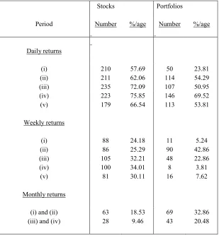
Table 2 contains a summary of the numbers of stocks and portfolios with skewed returns according to the skewness component of the Bera Jarque test. The first panel summarises the daily values from Table 1. The second panel shows the corresponding numbers for weekly returns for each of the 5 periods. The third panel shows the number of skewed stocks for periods (i) and (ii) and (iii) and (iv) based on four-weekly data. The table confirms a well-known stylised fact of empirical data; the incidence of skewness tends to decline as the frequency of the data decreases.

To investigate the potential for the use of the RL-beta and to compare it with the standard beta based on the market model, the following analysis was carried out for each of the five non-overlapping time periods for both stocks and portfolios. The standard market model was estimated for each stock (portfolio) using excess returns defined in the usual way. The RL-beta was also estimated using the regression method described in Section 5. The two approaches were compared using Hotelling’s test. The results from these investigations for stocks for period (i) ending on 3rdNovember 2003 are shown in Table 3. The corresponding results for portfolios are shown in Table 4.

Table 3 about here

The results are grouped into percentiles by considering the p-values of Hotelling’s test. Thus, as shown in panel (i) of Table 3, 17 stocks have a p-value of 0.01 or less, 48 have a value of greater than 0.01 but less than or equal to 0.05 and so on. For the 17 stocks in the first column, panel (ii) shows that the median value of the probability associated with the skewness component of the Bera Jarque test is 0.0244 and panel (iii) shows that the average value is 0.1670. Panel (iv) gives average values for the estimated alpha in the market model and the average p-value. Panel (v) reports the same statistics for the alpha in the RL-beta model. Also shown in panel (v) for comparison purposes is the predicted value based on the approximate formula in equation (20.). Panel (vi) shows the average of the estimated betas and RL-betas and panel (vii) shows the average values of Hotelling’s test and the associated p-values.

in these columns, beta is a better measure of performance than RL-beta. For the other columns of the table, accounting for 299 stocks, for which the p-value associated with Hotelling’s test is greater than 0.05, there is no significant difference between the two measures.

There are several empirical results in Table 3 which merit some comment. First, as shown in panels (ii) and (iii), the probability associated with skewness in returns decreases as the one-tailed p-value of Hotelling’s test increases. Thus, for this data set, the presence of skewness in returns reduces the superiority of beta over RL-beta. However, even for the most skewed returns the positive average value of Hotelling’s test means that the RL-beta is never superior. Indeed, a detailed examination of the results failed to yield a single case where the value of Hotelling’s test is negative, which would have indicated a preference for RL-beta.

Secondly, the estimated alphas under the market model fail on average to achieve significance. By contrast, the estimated RL-alphas are on average significantly different from zero. There is also a close correspondence between the estimated values and the values predicted by equation (20.). The exception is the final column of the table, for which returns exhibit the most skewness. Finally, there is very close agreement between the two sets of estimated betas, thus confirming the theoretical predictions due originally to Leland (1999), as expanded in Section 3.

It is not the purpose of this paper to comment in detail on all of the results that have led to Table 3. However, it is interesting to note from panels (ii), (iii) and (vi) that increasing skewness in returns leads on average to a decreasing value of the estimated beta. This indicates that there is a need to reconsider both beta and RL-beta in the context of models with econometric specifications that take skewness into account.

Table 4 about here

Table 4 shows the comparable results for portfolios. The most striking difference between the two sets of results shown in Tables 3 and 4 is that for 184 portfolios out of 210 beta is a superior measure of performance than RL-beta. This finding is supported by the probabilities in panel (iii) which indicate that on average these portfolios do not exhibit skewness. However, the median values in panel (ii) indicate that beta may be better than RL-beta in some cases even in the presence of skewness as measured by the Bera Jarque test. The other conclusions that may be inferred from Table 4 are broadly similar to the findings reported for Table 3. In the interests of brevity, the corresponding results for period (ii) which ended on 3rd December 2001 are omitted. These are generally similar to those summarised above. For the earlier time periods, (iii) – (v), there is little evidence of significant differences between the two measures based on daily data.

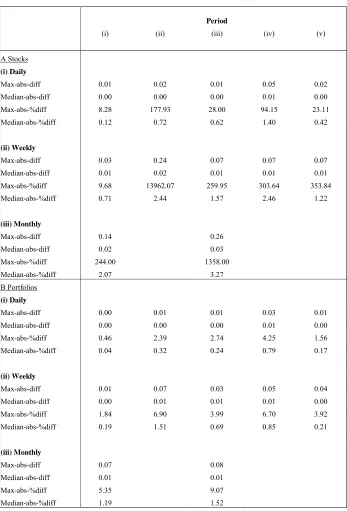
done for the two time periods. The table confirms that the differences between the estimated values of beta and RL-beta increase as the frequency of returns decreases. Inspection of the rows entitled “median-abs-diff” and “median-abs-%diff” make it clear that in general the difference between beta and RL-beta is small even for four-weekly data. However, as the rows entitled “Max” imply, there is a small number of stocks for which the difference is large. Detailed inspection of computed values of beta and RL-beta shows that these are stocks for which both estimates are numerically quite close to zero; that is they are more or less uncorrelated with returns on the market index.

Table 5 about here

7. Summary and Conclusions

It is shown that there are situations in which the theoretical values of the RL-beta will be similar to the traditional measure based on the CAPM. For the case where returns have a normal distribution, it is shown that either the RL-beta reduces exactly to the conventional beta or that it does not exist. It is therefore conjectured that the modified measure will be useful for portfolios which have non-symmetric return distributions. It is shown how to estimate RL-beta using regression and how to compare the resulting estimator with the traditional estimated beta using a test due to Hotelling (1940).

The empirical study is based on daily returns of UKFTSE350 stocks and on simulated portfolios of such stocks. The study provides some evidence for the period 2001-2003 that in the absence of skewness beta is to be preferred as a measure of risk. However, for the same period, even in the presence of skewness there is no evidence to suggest the superiority of the RL-beta. For earlier time periods, there is little evidence that indicates any statistically significant difference between the two models of risk regardless of the degree of skewness present in returns. The empirical results confirm one of the theoretical predictions, namely that when regression is used for estimation the variable used in the RL-beta induces a non-zero value of alpha. The empirical evidence supports the view that there will be larger differences at lower frequencies between the estimated values of beta and RL-beta. For most stocks, these differences are found to be numerically small. The data set studied in this paper leads to the inference that beta and alpha are still valid measures of risk and excess performance, at least when compared with RL-beta.

It is planned that further work in this area will investigate the application of the RL-beta to portfolios which contain stock options and which may therefore exhibit more extreme degrees of skewness.

Appendix A – Derivation of Equation 12

. , 1 1 1 1 2 1 2 1

exp 2 2

2 2 _say e e e e m pm m pm b b b b m m p p p           _{  }       __ __

Noting that _/ 2

m pm

p  

  the second term may be written as:

1 1 2 2     m m p b b e e    .

Expanding the numerator and denominator and assuming that terms in 2

m

 with powers higher than 1 may be ignored gives:

. , ) 1 ( 2 1 1 1 1 2 2 2 say b e e p p m p b b m m p         _{ }            

Using the assumptions of Section 3, equation (7.) may be written as:

               ) 1 ( 1 2 2 2 1 2 1 f p

f e R

R

ep p m m

 .

Dividing throughout by , expanding the exponential functions and ignoring terms with powers higher than two gives:



m f



p p p f

p R     R

 ,

where:







2 2 2 2



2 1 m m p p p

p     

     , and:







      _{  }  1 2 1

1 m f p

p  R 

 .

Appendix B – Hotelling’s Test

This is a test of the equality of correlation of a dependent variable Y with two independent variables, X1and X2. The aim is to select the independent variable that is

significantly more highly correlated with Y. Hotelling’s test proceeds as follows. First, standardise each X so that it has sample mean equal to zero and sample variance equal to one. In this appendix, the standardised variables will be denoted X1,2. For a

N X X r N i / 1 2 1 0



  .

Secondly, form two new independent variables defined as follows:

) 1 ( 2 , ) 1 ( 2 0 2 1 2 0 2 1 1 r X X x r X X x       .

The new variables have sample means equal to zero. In addition:





     N

i i i

N i ji x x j x

1 1 2 1

2 _{1, 1,2; 0 .}

Since the x1,2are linear transformations of the original variables, a regression of Y on

X1,2may be written as:

  

  

 1x1 2x2

Y

Hotelling shows that the OLS estimators of the three parameters are, respectively:





     N i i i N i i

ix Yx

Y Y 1 2 2 1 1

1 , ˆ

ˆ ,

ˆ  

 .

The null hypothesis of equal correlation is tested by the t statistic:

2 1 ˆ ˆ    t ,

where _ˆ2_{is the usual estimator of residual variance. The degrees of freedom are equal}

to N-3. Significant positive (negative) values of t indicate X1(X2).

References

Adcock, C . J. (1973) The Distribution Theory of Quadratic Forms With Applications, PhD thesis, The University of Southampton.

Adcock, C. J. (2004) Capital Asset Pricing for UK Stocks Under the Multivariate Skew-Normal Distribution. In Genton, M. ed., Skew Elliptical Distributions and Their Applications: A Journey Beyond Normality. Chapman and Hall. Boca Raton.

Breeden, D. and R. Litzenberger (1978) Prices of State Contingent Claims Implicit in Option Prices, Journal of Business, 51, p621-652.

Fang, K. T., S. Kotz and K.-W. Ng (1990) Symmetric Multivariate and Related Distributions, Chapman and Hall, London and New York.

Harvey, C. R. and A. Siddique (2000) Conditional Skewness in Asset Pricing Tests, Journal of Finance, 55, p1263-1295.

Hotelling, H. (1940) The selection of variates for use in prediction with some comments on the problem of nuisance parameters. Ann. Math. Stat., 11, p271–

283.

Isakov, D. and B. Morard (2001) Improving Portfolio Performance with Option Strategies: Evidence from Switzerland, European Financial Management, 7, p73-91.

Kallberg J. G. & W. T. Ziemba (1983) Comparison of Alternative Functions in Portfolio Selection Problems, Management Science, 11, p1257 – 1276.

Kraus, A. and R. H. Litzenberger (1976) Skewness Preference and the Valuation of Risk Assets, Journal of Finance, 31, p1085-1100.

Leland, H. E. (1999) Beyond Mean-Variance: Performance Measurement in a Nonsymmetrical World, Financial Analysts Journal, 55, p27-36.

Liu, J. S. (1994) Siegel’s Formula via Stein’s Identities, Statistics and Probability Letters, 21:247-251.

Mandelbrot, B. B. (1997) A Case against the lognormal distribution, in Fractals and Scaling in Finance : Discontinuity, Concentration, Risk (B. B. Mandelbrot, editor), p252-270, Berlin, Springer.

Michaud, R. O. (1998) Efficient Asset Management, Harvard Business School Press, Boston.

Naus, J. I. (1969) The distribution of the logarithm of the sum of two lognormal variables, Journal of the American Statistical Association, 64, p655-659.

Pratt, J. W. (1964) Risk Aversion in the Small and in the Large, Econometrica, 32, p122 – 136.

Rubinstein, M. (1976) The Valuation of Uncertain Income Streams and the Pricing of Options, Bell Journal of Economics, 7, p407-425.

Samuelson, P. A. (1970) The Fundamental Theorem of Portfolio Analysis in terms of Means, Variance and Higher Moments, Review of Economic Studies, 37,

p537-542.

Simkowitz, M. A. and W. L. Beedles (1978) Diversification in a Three Moment World, Journal of Financial and Quantitative Analysis, 13, p927-941.

Singleton J C and J Wingender(1986) Skewness Persistence in Common Stock Returns, Journal of Financial and Quantitative Analysis, 13, p335-341.

Stein, C. M. (1981)Estimation of the Mean of a Multivariate Normal Distribution, Annals of Statistics, 9, p1135-1151.

Sun. Q. and Y. Yan (2003) Skewness Persistence with Optimal Portfolio Selection, Journal of Banking & Finance, 27, p111–1121.

Treynor, J. L. and K. Mazuy (1966) Can Mutual Funds Outguess the Market? Harvard Business Review, 44, p131-136.

Table 1 – Analysis of Skewness and Kurtosis for Daily Returns on FTSE350 Stocks and Portfolios

Based on daily returns on FTSE350 non-financial stocks from 5th_{April 1994 to 3}rd_{November 2003}

Individual stocks Portfolios

(i) From 04/12/01 to 03/11/03

Not-kurtotic Kurtotic Total Not-kurtotic Kurtotic Total

Not-skewed 0 154 154 3 157 160

Skewed 1 209 210 0 50 50

Total 1 363 364 3 207 210

(ii) From 04/01/00 to 03/12/01

Not-kurtotic Kurtotic Total Not-kurtotic Kurtotic Total

Not-skewed 4 125 129 12 84 96

Skewed 0 211 211 0 114 114

Total 4 336 340 12 198 210

(iii) From 03/02/98 to 03/01/00

Not-kurtotic Kurtotic Total Not-kurtotic Kurtotic Total

Not-skewed 1 90 91 4 99 103

Skewed 0 235 235 0 107 107

Total 1 325 326 4 206 210

(iv) From 05/03/96 to 02/02/98

Not-kurtotic Kurtotic Total Not-kurtotic Kurtotic Total

Not-skewed 0 71 71 1 63 64

Skewed 0 223 223 0 146 146

Total 0 294 294 1 209 210

(v) From 05/04/94 to 04/03/96

Not-kurtotic Kurtotic Total Not-kurtotic Kurtotic Total

Not-skewed 10 80 90 57 40 97

Skewed 1 178 179 5 108 113

Total 11 258 269 62 148 210

[image:19.612.109.467.124.563.2]

Table 2 – Summary of the Number of FTSE350 Stocks and Portfolios Exhibiting Skewness

Based on daily and weekly returns on FTSE350 non-financial stocks from 5th_{April 1994 to 3}rd

November 2003, and on four-weekly returns from 22nd_{March 1996 to 3}rd_{November 2003.}

Stocks Portfolios

Period Number %/age Number %/age

Daily returns

(i) 210 57.69 50 23.81

(ii) 211 62.06 114 54.29

(iii) 235 72.09 107 50.95

(iv) 223 75.85 146 69.52

(v) 179 66.54 113 53.81

Weekly returns

(i) 88 24.18 11 5.24

(ii) 86 25.29 90 42.86

(iii) 105 32.21 48 22.86

(iv) 100 34.01 8 3.81

(v) 81 30.11 16 7.62

Monthly returns

(i) and (ii) 63 18.53 69 32.86

(iii) and (iv) 28 9.46 43 20.48

[image:20.612.112.421.136.473.2]

[image:21.612.108.473.124.586.2]

Table 3 – Comparison of Beta and RL-beta for Daily Returns on FTSE350 Stocks for the period 4thDecember 2001 to 3rdNovember 2003

Based on 500 daily returns on FTSE350 non-financial stocks.

< 0.01 (0.01,0.05] (0.05,0.1] (0.1,0.2] (0.2,0.3] (0.3,0.4] (0.4,0.5]

(i) Number of observations

17 48 39 43 83 103 31

(ii) Probabilities for skewness component of Bera Jarque Test (median values)

0.0244 0.0779 0.0106 0.0044 0.0032 0.0000 0.0000

(iii) Probabilities for skewness component of Bera Jarque Test (mean values)

0.1670 0.2861 0.2624 0.1902 0.1436 0.0500 0.0491

(iv) Estimated alpha in market model

Coefficient -0.0001 0.0000 0.0002 -0.0001 0.0001 0.0000 0.0000

P-value 0.6415 0.6377 0.6128 0.6052 0.5988 0.5507 0.4554

(V) Estimated RL alpha

Coefficient -0.6068 -0.5884 -0.5053 -0.3939 -0.3189 -0.1729 -0.0775

Predicted -0.6064 -0.5881 -0.5053 -0.3939 -0.3192 -0.1732 -0.0780

P-value 0.0000 0.0000 0.0000 0.0000 0.0000 0.0004 0.1889

(vi) Estimated market model and RL betas

MM 1.0982 1.0650 0.9151 0.7134 0.5780 0.3137 0.1412

RL 1.0983 1.0653 0.9151 0.7130 0.5774 0.3131 0.1402

(vii) Hotelling's Test

Test 2.6401 1.9614 1.4762 0.9903 0.6637 0.3903 0.1489

P-value 0.0051 0.0271 0.0714 0.1628 0.2545 0.3486 0.4409

[image:21.612.109.472.128.584.2]

[image:22.612.109.426.316.600.2]

Table 4 – Comparison of Beta and RL-beta for Daily Returns on Simulated Portfolios of FTSE350 Stocks for the period 4th December 2001 to 3rd November 2003

Based on 500 daily returns on FTSE350 non-financial stocks.

< 0.01 (0.01,0.05] (0.05,0.1] (0.1,0.2] (0.2,0.3] (0.3,0.4]

(i) Number of observations

155 29 12 9 4 1

(ii) Probabilities for skewness component of Bera Jarque Test (median values)

0.2379 0.0076 0.0082 0.3936 0.0006 0.0000

(iii) Probabilities for skewness component of Bera Jarque Test (mean values)

Bjskewp 0.3416 0.1725 0.1744 0.4096 0.0430 0.0000

(iv) Estimated alpha in market model

Coefficient 0.0001 0.0002 0.0000 -0.0003 0.0001 -0.0011

P-value 0.5051 0.6091 0.5837 0.4709 0.7728 0.3567

(v) Estimated RL alpha

Coefficient -0.4760 -0.3085 -0.2995 -0.2813 -0.1694 -0.2602

Predicted -0.4760 -0.3087 -0.2995 -0.2809 -0.1700 -0.2587

P-value 0.0000 0.0000 0.0000 0.0000 0.0000 0.0000

(vi) Estimated market model and RL betas

MM 0.8621 0.5591 0.5424 0.5088 0.3078 0.4685

RL 0.8619 0.5588 0.5420 0.5086 0.3069 0.4691

(vii) Hotelling's Test

Test 13.0681 1.9801 1.4586 1.0085 0.6968 0.5011

P-value 0.0008 0.0265 0.0737 0.1589 0.2439 0.3083

[image:23.612.110.457.113.624.2]

Table 5 – Analysis of the Difference Between Estimated Values of Beta and RL-beta.

Period

(i) (ii) (iii) (iv) (v)

A Stocks (i) Daily

Max-abs-diff 0.01 0.02 0.01 0.05 0.02

Median-abs-diff 0.00 0.00 0.00 0.01 0.00 Max-abs-%diff 8.28 177.93 28.00 94.15 23.11 Median-abs-%diff 0.12 0.72 0.62 1.40 0.42

(ii) Weekly

Max-abs-diff 0.03 0.24 0.07 0.07 0.07

Median-abs-diff 0.01 0.02 0.01 0.01 0.01 Max-abs-%diff 9.68 13962.07 259.95 303.64 353.84 Median-abs-%diff 0.71 2.44 1.57 2.46 1.22

(iii) Monthly

Max-abs-diff 0.14 0.26

Median-abs-diff 0.02 0.03

Max-abs-%diff 244.00 1358.00 Median-abs-%diff 2.07 3.27 B Portfolios

(i) Daily

Max-abs-diff 0.00 0.01 0.01 0.03 0.01

Median-abs-diff 0.00 0.00 0.00 0.01 0.00 Max-abs-%diff 0.46 2.39 2.74 4.25 1.56 Median-abs-%diff 0.04 0.32 0.24 0.79 0.17

(ii) Weekly

Max-abs-diff 0.01 0.07 0.03 0.05 0.04

Median-abs-diff 0.00 0.01 0.01 0.01 0.00 Max-abs-%diff 1.84 6.90 3.99 6.70 3.92 Median-abs-%diff 0.19 1.51 0.69 0.85 0.21

(iii) Monthly

Max-abs-diff 0.07 0.08

Median-abs-diff 0.01 0.01

Max-abs-%diff 5.35 9.07

Median-abs-%diff 1.19 1.52