THESES. SIS/LIBRARY R.G. MENZIES BUILDING N0.2 Australian National University Canberra ACT 0200 Australia
USE OF THESES
This copy is supplied for purposes of private study and research only. Passages from the thesis may not be copied or closely paraphrased without the
written consent of the author.
Telephone: "61 2 6125 4631 Facsimile: "61 2 6125 4063
Agricultural Labour Markets in India
Gaurav Datt
A thesis submitted for the degree of Doctor of Philosophy
Australian National University
January 1989
Declaration
Acknowledgements
My greatest debt is to my supervisors Drs R. M. Sundrum, Martin Ravallion and Anne Booth for their continued enthusiasm, guidance and patience!
I am grateful to the International Crops Research Institute for Semi-Arid Tropics (ICRISAT, Hyderabad, India) for allowing me to use their Village-Level Studies data set for the purposes of this study. ICRISAT, of course, bears no responsibility for the contents of this research.
I am also grateful to Drs Ashok Rudra, Tom Walker, Kaushik Basu, A. Vaidyanathan, D. P. Chaudhri, Jim Ryan, R. P. Singh, Abhljit Sen and Jurgen Eichberger for discussion of specific points. Special thanks is also due to Anand Swamy for lengthy discussions during my field trip to India. Dr John Beggs comments on the econometric work were extremely useful.
Fellow students at the Economics Department (RSPacS) have contributed in many ways. Special thanks to Ian Coxhead. Idris Sulaiman offered willing help with computer hardware problems.
Last but most, I am thankful to Geeta who not only
Abstract
The thesis is concerned with the problem of wage and
employment determination in the (casual) agricultural labour markets of India. It is argued that the extant theories of wage determination poorly accord with the stylized facts of the Indian situation. An alternative perspective on agricultural labour markets is developed, where wage determination at the village level is interpreted as the outcome of tacit collective bargaining between village labourers and employers. It is argued that cooperative behaviour, necessary to support such collective bargaining, can often be sustained through the operation of certain informal social sanctions against wage cutting behaviour.
With an asymmetric Nash framework, a theoretical model of the village-level market for agricultural labour is developed, which simultaneously determines the agricultural wage rate, the level of employment and the employers' profits. The model is consistent with the existence of involuntary unemployment, while also explaining variability of wages. In the extended version of the model, male and female labourers are introduced as separate bargaining parties. The extended model provides a possible explanation for the existence of gender wage (and employment) disparities.
Both the basic and extended models are econometrically estimated for ten villages in central, south and west India, using data collected by the International Crops Research Institute for Semi-Arid Tropics (Hyderabad).
Table of Contents
Declaration
Acknowledgements Abstract
Table of Contents
List of Tables and Figures
CHAPTER 1
Introduction
CHAPTER2
1.1 Motivation
1.2 The Point of Departure 1.3 Overview of the Study
Agricultural Wage and Employment Determination m India: A Review of Theory and Evidence
CHAPTER3
2.1 Introduction
2.2 'Subsistence' Wage Theories 2.3 Efficiency Wage Theory 2.4 Labour Turnover Models 2.5 Supply-Demand Models 2.6 Interlinked Markets Theory 2. 7 Conclusion
Village-Level Markets for Agricultural Labour and Tacit Collective Wage Bargaining
3 .1 Introduction
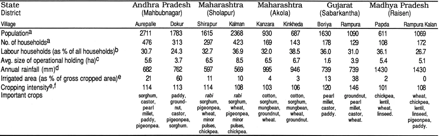
3 .2 The Study Villages
3 .3 Significance of the Casual Labour Market 3 .4 Incidence of Involuntary Market
Page 11 llI IV v IX 1 1 2 4 6 6 6 12 23 26 34
38
41 41 42 45Unemployment 4 6
3.5 Intra-village Uniformity of the Wage Rate 4 9 3.5.1 Operation- and Sex-specific Wage
Functions 5 3
3.6 Domain of the Labour Market and the
3.6.1 Rampura Kalan 3.6.2 Papda
3. 7 Theoretical Implications
3.8 Social Sanctions and Tacit Collective Bargaining in the Village Labour Market 3 .9 Some Further Observations
55 56 58
60 68 Appendix 3A
Sampling Fractions and Farm Size Categories in
the Study Villages 7 2
Appendix 3B
Village-, Operation- and Sex-specific Wage
Functions 73
Appendix 3C
Labour Market Questionnaire 79
CHAPTER4
A Bargain-theoretic Analysis of Agricultural Labour
Markets 8 2
4.1 Introduction 8 2
4.2 Nash and Other Bargaining Solutions 8 4
4.3 Symmetry versus asymmetry 9 1
4.4 The Basic Model 9 2
4.5 Comparative Statics: Basic Model 9 9
4.5.1 Change in employers' bargaining
power (~) 100
4.5.2 Change in labourers' alternative
earnings (v) 100
4.5.3 Change in fixed inputs (z) 101
4.5.4. Change in output or variable
(non-labour) input prices (p) 102
4.6 The Extended Model 103
4.7 Comparative Statics: Extended Model 107
4.7.1 Change in male labourers' bargaining
power (~M) 1 0 9
4.7.2 Change in female labourers' bargaining
power (~p) 111
4.7.3. Change in disagreement payoff of
male labourers (vM) 112
CHAPTERS
female labourers (vp) 4.8 Conclusion
114 116
Estimation of the Basic Wage Bargaining Model for
Indian Agricultural Labour Markets 11 8
5.1 Introduction 118
5.2 Specification of Functional Forms 118
5.3 Specification of Fixed and Variable Inputs 122
5.4 Specification of Disagreement Payoffs 125
5.6 The Wage Equation Again: Relaxing Risk
Neutrality 129
5. 7 Data, Variables and Measurement 1 3 0
5.8 The Econometric Model and Estimation 13 5
5.8.1 Single Equation Estimation and Testing
for Endogeneity of Wage Variables 1 3 6 5.8.2 Simultaneous Equation Estimation and
Testing for Cross-equation Restrictions
5.8.3 Testing for Zero Parameter Restrictions
5.9 The Preferred Estimates and Discussion 5.9.1 The Labour Demand Function 5.9.2 The Bargained-Wage Equation 5.10 A Sensitivity Analysis of the Bargaining
Power Coefficient
139
143 145 147 148
149 Appendix 5A
CHAPTER6
Testing for Heteroskedasticity and Implications
for Estimation 152
Estimation of the Extended Wage Bargaining Model 15 6
6.1 Introduction 156
6.2 Econometric Specification of the Extended
Model 159
6.3 The Data Set 16 1
6.4 The Results and Discussion 1 6 2
6.4.1 Male and Female Labour Demand
6.4.2 Male and Female Wage Equations 16 7 6.5 Sign Conditions for Comparative Static Effects 16 8
6.6 Conclusion 16 9
Appendix 6A
Operation-specific Modal Wage Rates for Male and
Female Labourers 1 7 2
CHAPTER 7
Seasonality, Regional Effects and the Distributional Consequences of Unequal Bargaining Power: Some Extensions and Simulations
7 .1 Introduction
7 .2 Seasonal Variations 7 .3 Regional Variations
7.4 Bargaining Power Asymmetry and
178 178 179 184
Implications for Income Distribution 1 8 8
7 .5 Disagreement Payoff Effects 1 9 0
7 .6 Output Price Effects 1 9 3
7. 7 Effects of Cropping and Irrigation Intensity 1 9 5 7 .8 Gender Inequalities in Bargaining Power and
Distributional Implications
CHAPTERS Conclusion
8 .1 The Suggested Characterization 8.2 The Theoretical Model
8.3 Empirical Quantification of Relative Bargaining
197
200 200 201
Power 202
8.4 Implications of Unequal Bargaining Power 204
8.5 Scope for Further Work 205
List of Tables and Figures
Table 2.1: Indices of Real Wage Rates for Male Agricultural Labourers Based on the Agricultural/Rural Labour
Page
Enquiries and the National Sample Survey Data 11
Table 2.2: Pattern of Male Employment in Rural India:
1972-73 and 1982-83 1 7
Table 2.3: Paired t-tests of Mean Differences between Probabilities of Employment and Wage Rates for Labourers from Landless, Small and Medium Farm
Households 2 0
Table 2.4: Incidence of Unemployment m Daily Hired Labour Markets of Six Villages in Central and South India,
1975-76 33
Table 2.5: Loans From Employers as a Proportion of Average
Debt per Indebted Agricultural Labour Household 3 8
Table 3 .1: Some General Characteristics of the Study
Villages 4 3
Table 3 .2: Average Composition of Annual (Hours of) Farm
Labour Use 4 5
Table 3.3: Incidence of Involuntary Market Unemployment
Among Labour and Small Farm Households 4 7
Table 3.4: Rates of Involuntary Market Unemployment Among Labour and Small Farm Households in Different Years
Table 3.5: Within-village Uniformity of the Hourly Wage Rate for Pre-harvest (and Harvest and Post-harvest) Operations
49
Table 3A.1: Sampling Fractions in the Ten Study Villages 7 2
Table 3A.2: Farm Size Classification Based on Operational
Land Holdings in the Study Villages 7 2
Table 3B.1: Operation-specific Wage Functions Male Hired Labour
Table 3B.2: Operation-specific Wage Functions
74
Female Hired Labour 7 5
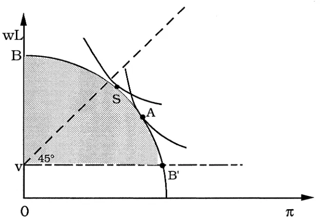
Figure 4.1: Nash and Kalai-Smorodinsky Solutions 8 8
Figure 4.2: Symmetric and Asymmetric Nash Solutions for
the Village Labour Market 9 6
Table 4.1: Signs of Comparative Static Effects: Basic Model 103
Table 4.2: Direction of Comparative Static Effects: Extended Model
Table 5 .1: Summary Statistics for Model Variables
Table 5.2a: Single Equation Parameter Estimates: The Profit
115
135
Function 1 3 7
Table 5.2b: Single Equation Parameter Estimates: The Labour
Demand Function 1 3 8
Table 5.2c: Single Equation Parameter Estimates: The Wage Function
Table 5.3: The Wu-Hausman Test for Endogeneity of Wage Variables
Table 5.4: Heteroskedasticity-corrected NL3S Estimates with Cross-equation Restrictions
138
139
Table 5.5: NL3S Estimates with Zero Parameter Restrictions 144
Table 5.6: The 'Preferred' NL3S Parameter Estimates 146
Table 5. 7: Estimated Elasticities of Hired Labour Use 1 4 8
Table 5.8: Estimated Parameters of the Wage Function for Different Values of the Employers' Disagreement
Payoff 151
Table 5A.1: NL3S Estimates with Cross-equation Restrictions
Uncorrected for Heteroskedasticity 15 4
Table 6.1: Average Male-Female Wage Rates and Composition of Annual Hired Labour Use
Table 6.2: Summary Statistics for Additional Model Variables
Table 6.3: NL3S Estimates of the Extended Model
157
162
Parameters 164
Table 6.4: Estimated Elasticities of Male and Female Hired
Labour Use 166
Table 6.5: Direction of Comparative Static Effects for the Extended Model on the Basis of Parameter Estimates
Table 6A.1: Modal Wage Rates for Male and Female Labourers: Aurepalle
Table 6A.2: Modal Wage Rates for Male and Female Labourers: Dokur
Table 6A.3: Modal Wage Rates for Male and Female Labourers: Shirapur
Table 6A.4: Modal Wage Rates for Male and Female Labourers: Kalman
Table 6A.5: Modal Wage Rates for Male and Female
169
172
173
173
Labourers: Kanzara
Table 6A.6: Modal Wage Rates for Male and Female Labourers: Kinkheda
Table 6A.7: Modal Wage Rates for Male and Female Labourers: Boriya
Table 6A.8: Modal Wage Rates for Male and Female Labourers: Rampura
Table 6A.9: Modal Wage Rates for Male and Female Labourers: Papda
Table 6A.10: Modal Wage Rates for Male and Female Labourers: Rampura Kalan
Table 7 .1: NL3S Parameter Estimates for the Season-augmented Model
Table 7 .2: NL3S Parameter Estimates for the
Region-174
175
175
176
176
177
183
augmented Model 1 8 6
Table 7 .3: Regional Differences m Bargaining Power 1 8 8
Table 7.4: Simulated Effects of Symmetric Bargaining Power 1 9 0
Table 7 .5: Simulated Effects of a Change in Labourers' Nonfarm Wage Earnings (y)
Table 7.6: Simulated Effects of a Change m the Labourers' Disagreement Payoff
Table 7. 7: Simulated Effects of a Change m the Average Price of Agricultural Output
Table 7.8: Simulated Effects of Changes m Cropping and
192
193
195
Irrigation Intensities 195
Table 7 .9: Simulated Effects of Equal Bargaining Powers for
CHAPTER 1
Introduction
1.1 Motivation
This is a study of agricultural labour markets in
contemporary India. The importance of the subject need not be belaboured. Suffice it to note that agricultural labour households constitute about 30 percent of all rural households in India, account for 44 percent of all rural households in absolute poverty and 61 percent of total unemployed person-days in rural India. The
incidence of poverty amongst the agricultural labour households is about 60 percent. I For anyone concerned with poverty and
unemployment in India, the importance of the subject is more than obvious.
Equally obvious is the central question pertaining to the operation of agricultural labour markets in India, viz., how are wage and employment outcomes determined in these markets. In
particular, there is the key puzzle of agricultural wage determination, that is, explaining the coexistence of involuntary unemployment with substantial wage variability. A very large body of evidence on both these aspects has accumulated over the years. While recognition of the latter feature has encouraged researchers to look for explanations in supply-demand models of wage determination, the former aspect has invited theoretical attention on models incorporating some form of wage inflexibility. Yet, it would be a fair assessment of the state of the subject to say that we do not yet have a satisfactory working hypothesis on this issue. What seems to be required is a theoretical
1 Sundaram and Tendulkar (1985). The reported figures relate to the year 1977-78 and are based on data collected by the National Sample Survey (32nd round). Agricultural labour households are defined as those whose major source of income in the year
framework which does not depend on market clearance as an
equilibrium concept and yet allows wages to be responsive to labour market conditions, particularly on the demand side.
1.2 The Point of Departure
It is this basic issue of wage and employment determination that defines the central focus of the present study. The point of
departure for this study is an alternative characterization of the 'ideal-type' agricultural labour market in India, which, in essence, is based on the following three related propositions:
(1) The unit of analysis needs to be the village, since the latter, for all practical purposes, defines the (spatial) domain of agricultural labour markets.
(2) Within village-level labour markets, agricultural wage
determination can be viewed as the outcome of implicit collective bargaining between the groups of village employers and labourers.
(3) The wage, employment and profit outcomes of such implicit bargaining critically depend on the relative bargaining powers of employers and labourers.
The choice of the unit of analysis must of course be a function of the problem to be analyzed and its particular empirical context. Ultimately, the unit of analysis should be the locus where the main 'determining forces', relevant to the problem at hand, coalesce. Well-known features of Indian rural labour markets, such as intra-village uniformity and inter-intra-village variation of the wage rate (for a given operation and sex), strongly suggest that the locus of
'determining forces' is the village, rather than the household or the district or the state. It is an implicit contention of this study that
The idea that there exists some form of tacit collective bargaining for the wage rate is a stylization of the village labour market environment. Village-level studies have frequently noted the phenomenon of a 'going' wage rate in the village, which participants in the village labour market abide by, irrespective of known
differences in the productive abilities of workers, and which is not bid down inspite of unemployment. Yet, the 'going' wage rate is not invariant over time and appears sensitive to parametric shifts in
labour demand and supply, particularly the former. The present study argues that this 'going' wage can be interpreted as the 'agreed' wage, i.e., the wage rate mutually agreed upon by village employers and labourers. The 'agreement' is nevertheless tacit; in the typical village situation, there are no formal agencies to enforce such agreement. Hence, the notion of implicit collective bargaining.
The empirical analysis in this study is based on data
collected by the International Crops Research Institute for Semi-Arid Tropics (ICRISAT, Hyderabad, India) as part of its Village-Level
Studies (VLS) program. The ICRISAT data set relates to ten villages in central, south and west India, representing five distinct
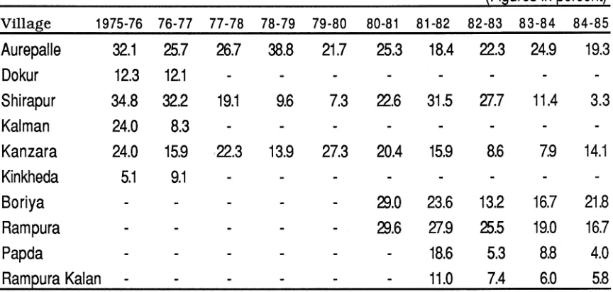
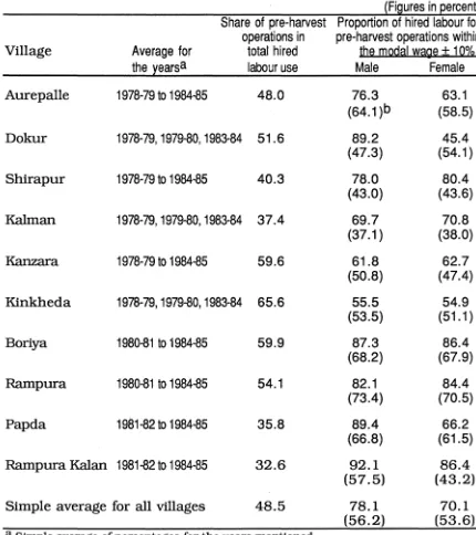
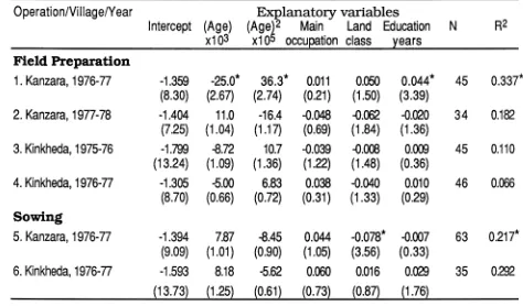
agroeconomic zones within India's semi-arid tropics.2 ICRISAT initiated its VLS program at six villages in Andhra Pradesh and Maharashtra in May 1975. The VLS coverage was extended to two more villages in Gujarat in 1980 and a further two villages in Madhya Pradesh in 1981. Altogether, the data set spans the period 1975-76 to 1984-85 covering a varying number of years for the ten villages.3
The decision to use the ICRISAT data set was based on the need (as noted above) to focus research at the village level. This data set appeared well-suited to the aims of the present study mainly in view of its large sample size per selected village (40 sample
households from different farm size categories were selected from
2 For further details on the selection of villages and ICRISAT's data collection procedures, see ICRISAT (1987).
each village) and its richness of detail on a wide range of aspects of the village agricultural economy. The data. having been collected at regular 2-4 week intervals. also provides year-round information.
1.3 Overview of the Study
Chapter 2 is a review of the theoretical and empirical literature. It is different from the usual 'literature review' chapter insofar as it focuses sharply on the key issue of agricultural wage determination. addressing in particular the question of how well the received theories of wage determination accord with the (stylized) facts of the Indian agricultural labour market situation.
Chapter 3 considers to what extent the features emerging from the review of chapter 2 also obtain in the ten study villages of the present study. The latter part of the chapter discusses the theoretical implications of the observed features. In particular. the argument is developed as to how quasi-cooperative forms of behaviour can arise in village-level labour markets even in a setting where
formal unions or other forms of explicit collusion are absent on either side of the market.
Chapter 4 goes on to model the village labour market within an asymmetric Nash bargaining framework. which explicitly allows for possible differences in the relative bargaining powers of village employers and labourers. The proposed model simultaneously
determines the agricultural wage rate. the level of employment and the employers' profits. An extended version of the model introduces male and female labourers as separate bargaining entities, and
analyses the joint determination of male and female wage rates and levels of employment along with the profits of the employers hiring them.
Chapters 5 and 6 are concerned with the empirical
labourers. And to test if the estimate provide any significant evidence of inequality of bargaining powers.
In chapter 7. I deal with some further aspects of agricultural labour markets within the framework of the estimated bargaining models. The first part of the chapter examines seasonal and regional variations in the relative bargaining positions of employers and
labourers. The second part of the chapter addresses the question whether the observed differences in bargaining powers are a
significant quantitative influence on distributional outcomes in the village economy.
CHAPTER2
Agricultural Wage and Employment Determination in India: A Review
of Theory and Evidence
2.1 Introduction
Despite the vast and growing body of literature on the operation of labour markets in the rural societies of less developed countries (LDCs), our understanding of the key processes of wage (and
employment) determination in these orbits of labour exchange
remains fragmentary. This chapter undertakes a critical review of the existing literature, focussing on the particular context of agricultural labour markets in India. The review is schematically organized in terms of the main theoretical approaches to the central issue of rural/agricultural wage determination, viz., (i) subsistence or institutional wage theories (section 2.2), (ii) efficiency wage
hypothesis (section 2.3), (iii) labour turnover models (section 2.4), (iv) supply-demand models (section 2.5), and (v) the interlinked markets theory (section 2.6). A major motivation for adopting this schematic framework has been to examine the extent to which the different paradigms of wage formation are compatible with the contemporary empirical reality of agricultural labour markets in India.
2.2 'Subsistence' Wage Theories
The idea that real wages in the LDCs are set at the
wages, I the basic elements of the classical wage theory may be listed
as follows2:
(i) Subsistence level is defined in terms of the real wage which supports zero population growth, where the rate of population growth is deemed to be an increasing function of the real wage.
(ii) There is a long-run tendency for real wages to conform to the subsistence level, the latter identified as the 'natural' price of labour.
(iii) The subsistence wage is, however, not a physiological datum, but also includes a cultural-historical element.3
(iv) The 'market' price for labour (the wages actually paid) usually differs from the 'natural' price (the long-run subsistence wage) depending on the supply and demand for labour.4
1 See Hollander ( 1984) for an exposition, and Samuelson's ( 1978) canonical classical model. Also see Booth and Sundrum ( 1984) for a somewhat different interpretation of Ricardian wage dynamics.
2This enumeration is based on a reading of Ricardo's (1911) chapter On Wages in The Principles of Political Economy and Taxation.
3 Even though Ricardo was quite explicit on this (in the chapter On Wages in the
Principles), the point remains contentious in view of the debate about whether real wages were assumed to influence population growth primarily through physiological factors related to mortality (O'Brien, 1981), or through psychological factors related to fertility (Hollander, 1979). Whatever be the historiographical significance of this exegetical problem, from the contemporary LDCs perspective the real issue (as
mentioned below) is that the assumed link between real wages and population growth is itself largely inoperative in the present-day context, and cannot be invoked as a wage-regulation mechanism.
4 Bharadwaj (1978) and Garegnani (1983) argue that the role of demand (and supply) in
Later, as demographic evidence burgeoned to show that there existed no straightforward monotonic relation between the rate of population growth and the real wage rate (or even real earnings), element (i) of the theory came to be disregarded. However,
dispensing with the demographic link implies that what remains of the 'subsistence' theory is simply the notion of general stability of real wages at some culturally and/or historically determined levels. The latter-day versions of the theory, which for the purposes of this discussion may be taken to include the so-called institutioned wage theories, can be broadly grouped into two categories. (1) The strong versions can be identified with fix-wage theories, where the wage refers to the real wage, and the wages are fixed not in the sense that they do not change but in the Hicksian sense that they are
independent of supply and demand. Included here are the
formulations which specify a perfectly elastic labour supply curve, the vertical height of the curve being exogenously determined.5 (2) The weak versions can be understood as postulating a long-term fixity of the real wage at the levels governed by some non-market forces, while permitting short-run influence of market forces of demand and
supply. The non-market forces may take the form of physiological and/ or sociological norms. 6, 7
the normal price not that of determining the latter, and that the market price is determinate only in its order relative to the normal price.
5 For such a view of subsistence theories, see, for instance, Hansen (1966). Squire (1981), Rakshit (1982) and Bardhan (1984a).
6 This interpretation is suggested by Lipton (1983), Binswanger and Rosenzweig (1984), Rodgers (1986) and Dreze and Mukherjee (1987).
7 It is worth noting that both the strong and the weak versions are compatible with the post-Sraffian view of the classical wage theory:" ... what all these authors [Smith, Malthus, Ricardo] had in common was not, as is often held, the idea of a wage
In the context of the LDCs, most of the empirical evidence presented against the subsistence theory has been targeted at the strong version. The critical thrust of this evidence has been the demonstration that the observed variation in the real wages is
attributable, in greater or smaller measure, to the supply and demand factors. See, for instance, Hansen (1966, 1969), K Bardhan (1973). Rosenzweig (1978), Bardhan (1979a,1984a,1984b), Squire (1981) and Lal ( 1986).
However, the weak version of the theory is not easily refuted. (By the same token, it is not easily verified either.) Like the strong version, it is not simply refuted by temporal or spatial
variation of real wages. But unlike the strong version, nor is it
necessarily refuted by the responsiveness of real wages to supply and demand factors. While the latter could be dismissed as ephemeral (short-term) phenomena, the former could be 'explained' in terms of temporal/spatial variability of non-market norms. However, in the absence of a supplementary theory of the determination and evolution of non-market norms, or additional structure linking short-term variation of real wages with their long-term constancy, it must be
concluded that the subsistence theory performs poorly on the criterion of falsifiability, and therefore, has very limited predictive power.s
The only prediction the weak version of the theory offers is regarding a long-term stability of real wages within reasonably
'homogeneous' spatial domains. Even here, it is not obvious just how long should the 'long-term' be. Nor is it altogether clear whether the
institutional kind) that are distinct from those affecting the social product and other shares in it, and are therefore best studied separately from them." (Garegnani, 1984, p. 295; Garegnani, 1983, p.311).
real wage rate or the real wage earnings of a labourer are relevant.9 The latter issue is clearly important insofar as unemployment is a widespread feature of rural labour markets in the LDCs. In the Indian agricultural labour market context, however, whether one considers the time-pattern of the real wage rates or real wage earnings, the evidence generally points against the subsistence/institutional wage theory.
Beginning with the evidence on real wage rates in
agriculture, first it ought to be recognized that studies using all-India averages (e.g. Lal, 1988) are not very meaningful, given India's
extreme regional heterogeneity. A minimal disaggregation would lead us to consider trends at the state level, for which there have been a large number of studies including Bardhan (1970), Krishnaji (1971), Hirway (1973), Jose (1974, 1984a, 1984b, 1988), Lal (1976a),
Nayyar (1976, 1977), Bhalla (1979), Ghose (1980), Kurien (1980), Parthasarthy and Adiseshu (1982), Kumar and Sharma (1983), Dey (1984), Mundie (1984a, 1984b) and Unni (1988). It is difficult to summarize the findings of these diverse studies insofar as they differ in their regional coverage, cover different time periods (though all of them relate to the post-independence period), and use different data sources. However, a detailed review of these studies is not presently contextual. The point I wish to emphasize is that (a) with a few
exceptions.IO these studies provide substantial evidence of significant (though diverse) regional trends in real agricultural wage rates, and
(b) even in regions where unidirectional movements in real wage
9 Ricardo's own numerical example involved annual wages of a labourer (Ricardo, 1911, p. 58). However, since Ricardo generally thought in terms of full employment (except for his chapter On Machinery), it mattered little whether wage earnings or the wage rate were considered.
10 The studies which note the absence of any significant trend include Nayyar (1977) for Bihar (1957-58 to 1971-72), Bhalla (1979) for Punjab (1961-62 to 1976-77).
rates are not sustained long enough to be interpreted as 'trends', the observed variations seem scarcely compatible with the notion of real wage rate stability. This is at least partially corroborated by the
figures in Table 2.1, based on the data source considered most
Table 2.1: Indices of Real Wage Rates for Male Agricultural Labourers Based on the Agricultural/Rural Labour Enquiries and the National
Sample Survey Data
State 1950-51 1956-57 1964-65 1974.75a 1977-78
Andhra Pradesh 110 100 101 86 120
Assam 133 100 101 71 na
Bihar 115 100 101 89 111
Gujarat * 100 124 83 118
Harayana ** 100 ** 72 **
Kerala 94 100 118 156 217
Madhya Pradesh 102 100 116 79 108
Maharashtra na 100 110 81 112
Karnataka 101 100 98 88 106
Orissa 83 100 110 79 106
Punjab 86 100 77 95 113
Rajasthan 103 100 132 97 128
Tamil Nadu na 100 118 105 146
Uttar Pradesh na 100 74 93 117
West Bengal 114 100 93 72 93
All-India 108 100 102 96 118
* included under Maharashtra
** included under Punjab na. Not available.
a. 1974-75 was not a good agricultural year. But as Bardhan (1985) observed, between 1964-65 and 1974-75, net foodgrain production increased by 20 percent and real NDP from agriculture increased by 11 percent.
reliable by researchers, 11 viz., the Agricultural and Rural Labour Enquiries and the National Sample Survey (NSS), even though it provides observations at only a few discrete points.
As for wage earnings of agricultural labour households in different regions, no time-series data are available. There are studies such as Jose (1978), Ghose (1980), Bardhan (1985) and Unni (1988) based on a few data points (spread over the period 1950-51 to
1977-78) provided by Agricultural and Rural Labour Enquiries and the NSS. Of course, no conclusions regarding trends can be drawn from these studies. However, they do suggest that (real) annual wage earnings per agricultural labour household (or per agricultural
labourer) have not remained constant in most regions.12 If anything, the evidence suggests a decline in most areas upto the mid-70s (in some cases after an initial period of growth upto the mid-60s), followed by some increase later.
2.3 Efficiency Wage Theory
It was noted that the subsistence/institutional wage theory (except in its classical incarnation) postulated rather than explained wage rigidity. The class of models that we consider in this section,
viz., the efficiency wage models, have sought to provide explanations for wage rigidities (strictly speaking, downward rigidity of real
wages) and the concomitant existence of involuntary unemployment. Following the original suggestion of Leibenstein (1957), the efficiency wage models were elaborated by Mirrlees (1975), Rodgers (1975). Stiglitz (1976, 1982), Bliss and Stern (1978a, b), Basu (1984, 1987a)
11 For a discussion of the relative merits of alternative data sources, see Rao ( 1972).
P Bardhan (1973), Lal (1976a), K Bardhan (1977) and Jose (1978).
12 This limited inference is certainly plausible unless it can be somehow argued that the six data points covered in these studies (viz. 1950-51, 1956-57, 1963-64/ 1964-65,
and Dasgupta and Ray (1986, 1987).13 The basic axiom underlying these models states that labour productivity or the effort per labourer (or per unit of time) positively depends on the real wage received by labourers.14 Given this basic relation, the efficiency wage models demonstrate that sufficient conditions are provided for employers wanting to pay more than the market-clearing wage, thereby
inducing involuntary unemployment. The argument, in nutshell, is as follows.
Given the effort-wage relation, there exists a unique15 real wage, the efficiency wage,
we,
which maximizes profits for anemployer or employers. (This is also the wage which minimizes the cost per unit of labour effort.) If
we
is less than the market-clearing wage, w5 (which also measures the supply price of labour), theemployers must pay w5 since no labourers will be willing to work for
an employer offering less than the market-clearing wage. However, if we exceeds w5, profit maximizing employers will clearly prefer to pay we, 16 Though labourers are willing to work for less, their supply price
13 See Akerlof and Yellen (1986) for a recent lucid survey of efficiency wage models, though oriented more to the context of labour markets in the developed countries. In contrast, the works mentioned above have been quite explicit in their contextual reference to the low-income countries.
14 Basu (1987a) has recently emphasized that in conjunction with this basic axiom, the efficiency wage models use another perception axiom whereby the positive wage-productivity link (or the basic axiom) is assumed to be fully perceived by each
employer.
15 Uniqueness. though not essential to the argument, is ensured by certain weak conditions on the effort-wage relation. See Bliss and Stem (1978a, p.334) and Dasgupta and Ray (1986,p.1018).
16 This does not necessarily conflict with competitive behaviour, for even under competitive conditions, employers always have the option of paying more than supply
ceases to be relevant for the employers. The equilibrium wage is thus given
w*= max
(we,
ws),and the efficiency wage sets a floor to the market wage (as also an upper bound to employment), which becomes operative whenever
we~ w5 • If the labour supply curve has the usual non-negative slope,
this saddles the system with involuntary unemployment which cannot be eliminated (through underbidding of the real wage) because
employers would only reduce their profits if they chose to pay anything less than
we.
Various microtheoretic justifications have been offered for the existence of a positive effort-wage relation, and it is indeed possible to develop a typology of efficiency wage models on that basis.17 However, in the context of developing countries, prime importance has been accorded to the nutritional determinants of labour effort; the nutrition-productivity linkage is presumed to be significant at low levels of consumption typical of these countries. The ensuing discussion is thus primarily geared to this latter class of nutritionally-based efficiency wage models.
The efficiency wage argument summarized above implicitly assumed a homogeneous set of labourers. It has, however, been
elaborated to consider one obvious dimension of heterogeneity among labourers, viz., their non-wage income based on their differing
17 For instance, Akerlof and Yellen (1986) use this approach to distinguish four broad types of efficiency wage models: (i) shirking models (e.g. Shapiro and Stiglitz,
1984) which emphasize that higher wages reduce shirking by employees due to a higher cost of job loss; (ii) adverse selection models (e.g. Weiss, 1980) focussing on the potential screening effect of higher wages in improving the average quality of job applicants; (iii) sociological models (e.g. Akerlof, 1982) which highlight the positive
effect of higher wages on the morale or the loyalty of the workers to the firm; and (iv)
(though limited) ownership of land. The basic distinction thus projected is between landless labourers and labourers with some land.18 The literature discusses both the competitive and
monopsonistic cases.19 Both cases may induce involuntary
unemployment in equilibrium, but they carry different implications for landed and landless labourers.
The non-competitive case turns on the familiar idea of discriminating monopsony, and shows that the landed labourers will be paid a lower wage than the landless as the employer seeks to equate the marginal cost of labour effort from the two sources (see Bliss and Stern, l 978a). This prediction is reversed in the
competitive case.20 It is shown that while the market for labour-effort
clears, there may be considerable invoiuntary unemployment of
labour-time (regimes 1 and 2 in Dasgupta and Ray, 1986). Also, while everyone employed earns the same (market-clearing) rate per unit of labour effort, those with non-wage income (viz. the landed labourers) earn a higher wage per unit of time. This is because labourers with non-wage income are potentially more attractive for the employers insofar as they can supply more effort than the landless labourers for the same time-wage. However, as employers compete for the services of such landed labourers, the time-wage for the latter is bid up. It is notable that the landed labourers enjoy an employment advantage over the landless in both the competitive and non-competitive cases.
The empirically attractive feature of the efficiency wage models lies in their ability to explain involuntary unemployment while also permitting (when the efficiency wage is not binding),
18 Though the literature concentrates on the landed-landless dichotomy, the
arguments also apply mutatis mutandis to other aspects of labour heterogeneity, such as differential dependency ratios.
19 The distinction between competitive and non-competitive market environments becomes analytically significant once labour heterogeneity in terms of additional sources of consumption is introduced.
responsiveness of wages to supply and demand forces.21 However, the mere existence of involuntary unemployment (and malnutrition) in rural labour milieus of LDCs can hardly be claimed a vindication of the efficiency wage hypothesis, as other explanations can be offered for these phenomena. We need to focus on specific assumptions and predictions of the theory to examine its empirical relevance.
The first point to be made is that the consumption-productivity link is far from instantaneous. And hence, if the
efficiency wage theory is to be considered a significant explanation of wage formation in rural labour markets, one would expect it to be supported by the prevalence of long-term employment contracts, which allow sufficient time for employers to capture the productivity benefits of paying higher wages. However, a striking feature of Indian agriculture is the preponderance of casual labour contracts, mostly on a daily wage basis.22 As shown in Table 2.2, for male labourers, casual employment accounts for nearly three-fourths of all wage
employment in rural India. The proportions for females (not reported in the table) are even higher since their participation in the regular or attached labour market is more limited. The NSS, 32nd Round data for 1977-78, indicate that the share of casual in total wage employment for male and female agricultural labourers were 76 and
21 For instance, seasonal variation of wages is quite consistent with the efficiency wage theory. A point overlooked by Hart (1986a, chapter 7) in her criticism of the theory in the Indonesian context.
94 percent respectively.23 Furthermore, figures in Table 2.2 are indicative of not just a high but an increasing rate of casualization of labour contracts. It should also be stressed that casualization is a country-wide phenomenon: all states show an increase in the proportion of casual labour over the 10-year period. If, thus, the efficiency wage
Table 2.2: Pattern of Male Employment in Rural India:
1972-73 and 1982-83
Wage labour as Casual labour as percentage percentage of total employment of wage labour
State 1972-73 1982-83 1972-73 1982-83
Andhra Pradesh 40.0 46.6 68.6 74.2
Assam 23.8 35.9 40.0 49.0
Bihar 39.5 42.8 60.9 82.2
Gujarat 34.4 40.4 64.6 81.5
Harayana 24.0 30.0 40.3 52.3
Kerala 54.3 54.5 72.1 76.7
Madhya Pradesh 27.3 33.7 56.8 72.0
Maharashtra 53.5 47.4 70.3 71.5
Karnataka 37.8 41.5 72.1 87.3
Orissa 39.9 43.7 68.3 76.8
Punjab 30.7 33.6 52.3 61.7
Rajasthan 10.2 20.5 53.5 63.1
Tamil Nadu 42.4 54.2 60.0 75.1
Uttar Pradesh 21.6 24.1 66.7 73.6
West Bengal 48.1 50.4 na 75.4
All-India 34.1 39.6 64.6 72.8
na. Not available.
SOURCE: Parthasarthy (1987), based on NSS, 27th Round, Sarvekshna, October 1977 and NSS, 38th Round, Report No. 315.
23 See Vaidyanathan (1986, 1988). Also see Binswanger et. al. (1984) who reported that the regular farm servant market in central and south Indian villages is almost
theory is considered applicable primarily to the category of regular or attached farm labourers, then it must be admitted that its relevance is limited to a small and shrinking segment of the agrarian labour market in India. 24
Basu (1987 a) has recently sought to restate the efficiency wage hypothesis for a casual labour market where the productivity-augmenting effects of wages paid by individual employers are allowed to enter their respective profit calculations only to the extent they are able to retain labourers with them. The model does exhibit the possibility of involuntary unemployment in equilibrium. However, if the rate of employee retention per period is rather small, as seems highly plausible in the daily-rated market (see note 22), the model collapses to the competitive supply-demand framework with
involuntary unemployment tending to disappear from the model altogether.
As suggested above, once labour heterogeneity is admitted into analysis, the efficiency wage theory offers more concrete
predictions, viz., (i) landed labourers (or those with some additional source of consumption) have a higher probability of finding
employment in the wage labour market than the landless, 25 and (ii) wage rates for the two categories are different, being higher (lower) for labourers with land if the labour market is competitive
(monopsonistic). However, these predictions accord poorly with the Indian situation. As for (i), the Rural Labour Enquiry (1974-75) data
24 The above evidence contrasts with Rodgers' (1975) findings for the Kosi region of Bihar that " a proportion, ranging upto nearly a half, of the labourers were 'tied' to some extent". The Kosi area could well be a somewhat special case. However, a closer look at Table 1 in Rodgers (1975) shows the proportions of 'tied' labourers in the 5 surveyed villages were 33, 46, 22, 20 and zero percent respectively, with a simple average of 24.2 and a high standard deviation of 15.2. The latter set offigures are much less propitious for the efficiency wage theory.
25 Notice the strong result in Dasgupta and Ray(l986) that under regime 1, none of the landless succeed in obtaining any employment, and in regime 2 involuntary
show that both male and female agricultural labourers from landed households faced a lower average probability of wage employment than those from landless households:
PROBABLITY OF WAGE AGRICULTURAL LABOUR
EMPLOYMENT IN HOUSEHOLDS
AGRICULTURE 26 WITHOUT LAND
for men 0.733
for women 0.569
AGRICULTURAL LABOUR HOUSEHOLDS
WITH LAND
0.693 0.498
A similar finding was also reported by Sinha (1981).27
Table 2.3 presents further evidence at a more micro-level for villages in the semi-arid tropics of Andhra Pradesh and
Maharashtra. It shows a mixed picture. The differences between the probability of market employment for landless and cultivator
households are as often positive as they are negative. They are significant in only about half the cases. Among the significant cases, higher probability for cultivator households is borne out for females only; for males the reverse appears to be true.
As for wage differences, Table 2.3 shows these to be mostly insignificant for females; for males, it suggests higher wage rates for cultivator households in accordance with the competitive version of the efficiency wage theory.28 In contrast, the wage functions
estimated by Rajaraman (1986) for two Karnataka villages found the land operated variable positive and significant for females, but
26 The probability of wage employment is calculated as the number of days in wage employment as a proportion of the sum of days in wage employment and days unemployed due to want of work.
27 See the evidence on unemployment cited in section 2. 5 below.
28 A disquieting feature of Table 2.3 is that wage differences often go in the opposite
insignificant for males in one village and negative and "not insignificant" in the other. Bardhan (1979a) also reported a significant negative coefficient for land in the daily farm wage
function estimated for West Bengal, in line with the non-competitive version of the efficiency wage theory though he himself favoured an alternative
Table 2.3: Paired t-tests of Mean Differences between Probabilities of Employment and Wage Rates for Labourers from Landless, Small and
Medium Farm Households
Landless - Small Farm
Village Probability of market employment Wage Rate
male female male female
Aurepalle -0.23 0.49 -2.16* -4.21 **
Dokur 0.33 1.45 0.60 -0.93
Shirapur -2.42* -8.21 * -2.18* -0.09
Kalman 2.97** -3.35** -5.79** 0.51
Kanzara 0.41 2.06* -6.33** 1.89
Kinkheda -6.79** -2.15* 1.52 1.68
Landless - Medium Farm
Village Probability of market employment Wage Rate
male
Aurepalle 2.05
Dokur -0.64
Shirapur 2.14*
Kalman 2.85**
Kanzara 1.61
Kinkheda 4.01 **
* significant at the 5% level:
** significant at the 1 %.
female male female
0.64 -0.58 -1.12
-3.17** 1.59 0.48
-3.95** -0.98 -1.99
-5.57** -1.46 3.87**
1.22 -4.13** -0.14
0.03 3.04** -1.46
Note: Probability of market employment is defined as the number of days a person was successful in obtaining wage employment as a proportion of the number of days (s)he tried.
explanation.29 Rosenzweig (1984), on the other hand, using national survey data of the National Council for Applied Economics Research (1970-71), found the amount of land owned by the worker to be insignificant in both the male and female wage equations.
It may be tempting to suggest that these diverse results are all consistent with the efficiency wage theory, and simply reflect competitive or monopsonistic market conditions obtaining in
different regions. However, in the absence of an independent study of the market structures in these regions, such ex post deduction would be clearly tautological. In my view, not much can be concluded on the basis of the reported wage differences among individual labourers since they are likely to reflect mainly non-individualistic aspects of wage variation, such as, inter-village differences or different rates for different agricultural operations. This is indeed what is suggested by the widely-documented evidence for intra-village uniformity of wage rate (for a given operation and labourers of the same sex).30 That, however, still leaves an unresolved problem for the efficiency wage theory, viz., how are uniform wages to be explained when sharp and readily observed productivity differences are known to exist among individual labourers in the same village labour market.
There has been little direct econometric testing of the efficiency wage hypothesis, presumably in view of the difficulties emphasized by Bliss and Stem (1978b).31 For India, the only attempt
29 This is discussed in greater detail in section 2.4. It is also noteworthy that in a similar regression for the monthly salary of regular farm labourers, Bardhan found a significant positive coefficient for the land variable.
30 See, for instance, Bardhan and Rudra (1981), Rudra (1982a,b, 1984), Bliss and Stern
(1982), Rodgers (1975), Rao (1984), Rodgers and Rodgers (1984), Ryan and Walker (1988), Dreze and Mukherjee (1987). Also see chapter 3.
31 Strauss (1986) tested the theory for Sierra Leone and found current nutrient intake
in this direction, to my knowledge, is by Behrman and Deolalikar (1986). They concluded:
Our results ... indicate significant support for the "Wage Efficiency hypothesis" for males within the rural SAT [semi-arid tropics] Indian context of this study, with significant differences between the peak and slack seasons.
However, a critical look at their results raises strong doubts whether any support at all can be claimed therefrom for the efficiency wage hypothesis.
To capture the efficiency-wage effects, Behrman and
Deolalikar included a weight-for-height measure and calorie intake as (instrumented) explanatory variables in the semilog wage equations estimated for male and female casual labourers.32 They also allowed peak season slope dummies for these two variables to capture inter-seasonal effects. However, in the estimated equation for female
participants, none of the four efficiency-wage variables were found to be significant. For males, only weight-for-height was found
significant, while calorie intake infact had a negative sign.33 Thus, even for males the case for efficiency wages rests on rather weak foundations. Further, the Behrman-Deolalikar explanation for the non-significance of efficiency-wage considerations for female labourers, in terms of male labour generally performing more physically-demanding tasks, also appears to be off the mark.
Particularly, when it is noted that women account for 50-88 percent of total hired labour in this region (see Ryan and Ghodke, 1984), and among the nine predominantly male operations are tasks such as watching, irrigating, plant protection and supervision (see Ryan and Walker, 1988, chapter 4).
Finally, as perceptively argued by Dreze and Mukherjee
32 I concentrate on the male and female wage equations rather than the combined one for all participants as the reported residual sums of squares would convincingly reject a Chow test on structural stability.
( 1987), efficiency wage models are flawed in a basic sense as a
relevant paradigm in the Indian context insofar as they attribute the resistance to wage cuts solely to the employers. There is considerable field-based evidence to suggest that the resistance to undercutting comes typically from .the labourers' camp.34 Among the employers, on the contrary, there is some evidence of resistance to overbidding of the wage rate (see Bliss and Stern, 1982).35
2.4 Labour Turnover Models
Labour turnover (hereafter L-T) models have the same basic structure as the efficiency wage models considered in section 2.3. Like the latter, they show that under certain circumstances
employers find it profitable to pay wages above the market clearing level. Such employer behaviour is, however, based, not on a positive effort-wage relation, but on an inverse relation between wages and the costs of labour turnover. Higher wages, it is argued, reduce
turnover costs either through a direct reduction in the workers' quit rate or by way of lowering the per worker replacement cost. In the context of LDCs, the original formulations of the L-T model, such as Stiglitz (1974), were intended as an explanation of the rural-urban wage gap (and urban unemployment). Later work, notably by Bardhan
(1979a), emphasized that L-T considerations were equally important for agricultural wage determination. Since Bardhan's work is
particularly addressed to the Indian context, it is considered in some detail below.
Bardhan (1979a) modeled36 a monopsonistic labour market
34This is most clearly documented by Rudra (1982a) and Bardhan and Rudra (1981).
Bliss and Stern (1982) and Dreze and Mukherjee (1987) also obseived this phenomenon for Palanpur.
35 This phenomenon has critical implications not just for the efficiency wage theory, and will be taken up again in section 2.5 as also in chapter 3.
36 Bardhan presented two versions of the L-T model, the second version incorporating
situation where the employer faces an exogenously given quit rate by workers.37 As existing labourers quit, the employer hires 'new'
labourers incurring in the process an average recruitment cost, c, over and above the usual wage cost. In particular, Bardhan introduced the following recruitment cost function
c = c(u, v),
decreasing in u '8.nd increasing in v, where u is the extent of unemployment in the village and v represents "any factor
constraining, and hence raising the average cost of recruitment on the part of the employer" (p. 492). Given this, the employer adjusts wages and employment to maximize profits. It is easily shown that involuntary unemployment typically characterizes the resultant equilibrium, and labourers cannot secure additional employment by bidding down the wage rate since a lower wage rate only serves to raise recruitment costs of the employer.
Bardhan also derived some comparative static propositions from the L-T model which indicate that (i) an exogenous increase in labour demand (due to such factors as improved agricultural
practices, a higher cropping intensity, better irrigation or rainfall, or simply a seasonal shift in demand for labour) increases the wage rate and lowers the unemployment, (ii) recruitment-constraining factors (such as those encumbering the supply of labour by landed labourers or those with low dependency ratios38) lower the wage rate and increase unemployment, and (iii) labourers with less elastic labour
discussion is confined to the first version, many of the remarks carry over to the second model as well.
37 This is in contrast to the L-T models proposed by Stiglitz (1974) and Salop (1979),
where the quit rate is endogenously determined. The difference, however, is not analytically significant since Bardhan makes the average turnover cost endogenous, while the other formulations take the latter to be exogenous.
supply get lower wages, while those with higher quit rates face greater unemployment. A measure of the empirical support is
claimed for these predictions. However, as observed in section 2.3,
the evidence for (ii),39 implying inter-worker wage differences in the same labour market, is generally inconclusive, and can sometimes be quite misleading.
The point also needs to be made that the comparative static results of Bardhan's model are contingent on some rather stringent assumptions on the recruitment cost function, viz., Cuu>O and Cuv=O. While there may be some intuition for the first derivatives of the recruitment cost function, 40 it is far from obvious what sort of
intuitive (or indeed empirical) support justifies the assumed signs of the second derivatives.41
A more fundamental problem with Bardhan's analysis in the Indian context relates to the concept of recruitment cost itself. A widely-observed feature of agricultural labour markets in India is that their territorial domain is essentially the village. 42 And within the village labour market, employers possess a higher degree of
knowledge of individual worker characteristics, including conditions of their labour supply. Labourers, on their part, are equally
well-informed of employers' labour requirements. Over the years, even
39 Bardhan cited evidence for West Bengal where he found a significant negative coefficient for land and a positive coefficient for dependency ratio in his estimates of wage function for casual labourers. See section 2.3 for relevant discussion.
40 For instance, it may be supposed that recruitment is more costly in tighter labour market conditions.
4l Yet IIlC!StJ>fBardhan's result~crittca1ly depend on the.aE;S!J.Il1e<:l signs. For exafi1ple,_
if Cuu< or =0 (which is a priori as plausible as Cuu>O) then exogenous increases in labour demand either have no effect or cause afaU in the wage rate. See Bardhan (1979a), p. 491.
42 See, for instance, Rudra (1982a), Bardhan and Rudra (1985, 1986), Sundari (1985)
seasonal fluctuations in labour use become a matter of common knowledge. In such a village environment, it is indeed hard to
visualize the kind of imperfections of information that could possibly form the basis of recruitment costs of L-T models.43
2.5 Supply-Demand Models
As discussed earlier (see section 2.2), contrary to the supposition of fix-wage theories, a large body of empirical evidence for rural labour markets in LDCs (including India) showed wages to be responsive to the varying conditions of demand for and supply of labour. Presumably on the strength of such evidence, research on rural labour markets witnessed, in contrast to the development literature of the 1950s and 60s, a renewed interest in supply-demand models, which (partially or fully) restored to wages (and prices) their Walrasian role of ensuring market clearance. For India, this is indicated by a number of studies including K. Bardhan (1970, 1973, 1977), Pandey (1973), Lal (1976b, 1988), Rosenzweig (1978, 1984), Vyas (1979), Papola and Misra (1980), Ryan (1982), Bardhan (1984a, b), Ryan and Wallace (1987).44 One could possibly distinguish on conventional lines between competitive and non-competitive
models; though it is the former that have been the focus of special attention.45
However, a characterization of India's agricultural labour
43 Bardhan himself comes close to admitting this in the concluding paragraph of his
paper. See Bardhan (1979a), p. 499.
44 Kalpana and Pranab Bardhan's work does not strictly belong to this class in view of their somewhat eclectic theoretical stance.
45 While monopsonistic labour market conditions have often been proposed in the
markets in terms of the competitive supply-demand framework is problematic on a number of counts. There is, first, the problem of the unit of analysis itself. This relates to the aforementioned village-level isolation of the labour market (see section 2.4), the clearest
manifestation of which is to be found in the persistent and significant differences in wage rates (for given operation and sex) even across adjacent villages. This is not to deny the existence of intra-rural labour migration, especially of a temporary seasonal type. However, while the phenomenon deserves further research, available evidence, such as Rudra (1982a), Breman (1985, particularly chapters 7 and
10) and Bardhan and Rudra (1986), indicates that rural circulation of labour is mostly across distant areas, is highly particularistic in being structured on personal ties, and is sometimes in 'perverse' direction from high to low-wage areas. 46 These features substantially inhibit the potential market-integrating effects of such movement even in
regions where it is quantitatively significant.
From the competitive theoretical perspective, however, territorial segmentation of the labour market per se need not be a problem, even as it implies the existence of (territorial) wage
differentials for similar work. There is indeed the view that "India is composed of a large number of geographically distinct, competitive rural labour markets" (see Rosenzweig, 1984, p.212). What is
problematic, though, is the situation that market segmentation
permeates right down to village level, where the rather small number of participants on either side of the market puts a heavy strain on the competitive assumption of price-taking behaviour (Rudra, 1984). This is further accentuated when we allow for elements of
non-substitutability between different types of labourers within the same village market, notably between attached and casual labourers, and among casual labourers between male and female labourers (Rudra,
1982b, chapter 15).
46 Bardhan and Rudra (1986) noted that 'pexverse' movement is not easily explained but suggested that "in most of these cases ties of familiarity, personal connections and trust, apart from the related credit nexus, may have been stronger than wage
A related problem stems from the observed within-village uniformity of the (task-specific) wage rate for casual labourers of the same sex, inspite of their widely-varying abilities which are also well-known in the village (see section 2.3). In the Arrow-Debreu
framework, labourers with different productive abilities would be treated as different commodities, but then there is no reason to expect identical equilibrium prices for these different
commodities.47 One may also question, in this context, the kind of empirical support for competitive wage determination that has sometimes been based on estimates of Mincer-type wage equations, for instance, by Ryan (1982), Ryan and Wallace (1987). The standard approach here is to regress wages (usually, natural logarithm of individual wages per period) on a vector of worker attributes. It is also common to add a few regressors to capture the effects of demand-side factors. The underlying theory is that the (hedonic) wage function reflects an equilibrium of supply and demand for labour at each level of worker attributes.48 Estimates of such wage equations for agricultural labourers in India have sometimes reported certain personal attributes to be significant,49 but not always so (see, for instance, Rosenzweig, 1984). It is hardly surprising that these exercises have found inter-village wage variation to be more important.
47 I thank Ashok Rudra for emphasizing to me the significance of this point. Also see Rudra (1984).
48 See the recent survey article by Willis (1986).
49 For instance, Ryan (1982) found years of schooling, age (proxy for experience) and indicators of physical and nutritional well-being to be important explanatory
variables in wage equations for male day-labourers in six villages of Andhra Pradesh and Maharashtra; these variables were insignificant in female wage equations. Using the same data set, Ryan and Wallace (1987) reestimated the wage equations correcting for the sample selectivity bias (discussed by Heckman 1974,1979) resulting from the fact that wage rates are observed only for those who worked. They obtained essentially
"In all equations it is clear that the village x agricultural year
dummies are explaining a substantial portion of the variation in wages of these participants"
.so
To the limited extent that the estimated wage equations do show intra-village wage variation, it is likely that a large part of it is simply task-wise variation, and the observed significant coefficients on worker attributes mainly reflect features of some employment-rationing scheme whereby different agricultural tasks get allocated among village labourers in different proportions.SI
A somewhat different empirical approach has been to estimate wage equations which are derived (explicitly or otherwise) as reduced-form specifications of the competitive market-clearing model, but do not necessarily include individual worker
characteristics among the set of regressors.S2 However, the basic point to emphasize about all these wage function studies (both Mincer-type and others) is that, at most, they establish a certain degree of sensitivity of wages to an exogenous set of supply and demand factors. To assert that they also thereby validate the
competitive (supply-demand) model of wage determination is a non-sequitur; the reduced-form wage equations of these studies tell us absolutely nothing about whether the labour market clears or not.
Other studies which jointly estimate labour supply and
demand functions within a simultaneous equation framework scarcely do any better. Rosenzweig (1984),S3 for instance, used district level
SO Ryan (1982), p. 33. The same also noted by Ryan and Wallace (1987).
Sl That such employment-rationing schemes do infact exist in village situations is, perhaps, best exemplified by the widely-observed gender-based division of
agricultural tasks. See for instance, Gulati (1978), Mencher and Sardamoni (1982), Agarwal (1984), Rudra (1982b), Rao (1984), Banerjee (1985), Bhati and Singh (1987) and Ryan and Walker (1988).
S2 See, for instance, Pandey (1973), Papola and Misra (1980) and Lal (1988).
data (of the Directorate of Economics and Statistics, and the Census of India, 1961) to estimate labour supply and demand functions
derived from a detailed competitive model of the rural labour market. It is claimed that the "empirical results ... were generally consistent with this framework" (p. 240). Scanning through the results, one finds that the only basis of this claim are the correct 'negative' signs on labour-supply variables in the wage equations (estimated
simultaneously with labour demand equations using full-information maximum-likelihood methods). Even here, "the negative supply effects of males and children on their respective wages [were] not statistically significant" (p. 229). However, the basic shortcoming of the exercise (as a test of the supply-demand model) is that the
estimation framework imposes competitive market clearance rather than testing it.54 The issue of unemployment is completely ignored.55 It can be argued that even the results that Rosenzweig does present are vitiated by the measurement error in labour supply variables on account of their being axiomatically equated with the observed levels of employment.
Bardhan's (1984) study for West Bengal adopted a more unusual approach in proposing the following simultaneous system for estimation:
(1) Ls = Ls (w, X)
(2) Ld = Ld (w, Z)
where Ls, Ld, w have their usual meaning, and X and Z are vectors of exogenous variables. However, instead of the standard market
54 It cannot be overemphasized that the distinguishing feature of the competitive model is not that labour supply and demand are functions of the wage rate, but that the wage rate adjusts more or less rapidly to clear the market. What is indeed subjected to some detailed testing in Rosenzweig (1978, 1984) are the properties of neoclassical labour supply functions, but that is hardly the same as testing the competitive model of the labour market.