Consequences of Sulfate reduction in Floodplain Wetlands

(1)

Consequences of Sulfate

Reduction in Floodplain Wetlands

By

Andrew Higgins

Submitted in fulfilment of the requirements for the degree of Master of Philosophy

(2)

(3)

Candidate's Declaration

This thesis contains no material which has been accepted for the award of any other degree or diploma in any university. To the best of the author’s knowledge, it contains no material previously published or written by another person, except where due reference is made in the text.

(4)

Acknowledgements

I didn’t do this alone. I am a better person for knowing and working with each of the following

people:

Firstly, I need to thank my supervisors Dr Sara Beavis, Prof David Ellis and Dr Paul Shand.

Their patience and guidance through difficult times is greatly appreciated.

Dr Andy Christy is thanked for his generosity, time and intellect. He could always say what I

couldn’t, in a way that I can’t. Dr Ulli Troitzsch was especially kind and helpful and I learned so

much from her.

I must thank Dr Sue welch for letting me know I was heading in the right direction and

encouraging me as a student to pursue research…..and the brownies.

Linda Mc Morrow, Brian Harrold and Nigel Craddy are thanked for their patience and help with

technical issues. Nigel is especially thanked for the torment, Brian for fixing my laptop without

making me feel stupid, and Linda for her advice with laboratory procedures and lab etiquette.

Fern Beavis was an incredible help on a field trip, and Luke Wallace is thanked for his advice and

his help with laboratory methods, as well as his endnote library.

Bear McPhail for letting me use his equipment.

This research was supported through scholarships and grants from the Research School of Earth

Science, the Australian National University, and the CSIRO’s Water for a Healthy Country

(5)

Abstract

This research project has been a laboratory based experimental study on the

cycling of sulfur in acid sulfate soils and underlying sediments of floodplain

wetlands. Of particular focus was the effect that the reductive transformations

of sulfur can have on nitrogen and phosphorus cycling. The objectives of this

study were to quantify the rates at which sulfidic material forms, the controls

on these rates, and to analyse the nutrient pulse from the sediments under a

low redox potential.

In-vitro experiments simulating inundation were conducted on sediments

collected from three wetlands of the Lower River Murray. Two were salt

disposal basins and another was a freshwater wetland. Experimental data

collected indicates that significant amounts of nitrogen and phosphorus will be

released from the sediments when inundated and anoxia is induced. The pulse

of nutrients from the sediments related to the geochemistry of the sediments,

as well as the hydrological regime. Partial drying and oxidation of sulfidic

material results in the formation of poorly crystalline iron (oxyhydr)oxide

minerals, which sorb phosphorus, with reductive dissolution following

inundation liberating sorbed phosphorus. The high calcium concentrations in

the salt disposal basins can potentially occlude the phosphorus through the

formation of apatite minerals. The result is that phosphorus is limiting primary

production in salt disposal basins and nitrogen is limiting in the freshwater

systems.

The pulse of nitrogen and phosphorus has the potential to increase algal

growth. Consequently, the increased algal growth and subsequent availability

of energy sources for microbial metabolism could increase the rate of sulfide

production. This research will enable land and catchment managers to better

(6)

List of Figures

Figure 2-1: Ecological Redox Sequence (Data from Stumm and Morgan (1996)). ... 8

Figure 2-2: Equilibrium distribution of sulfur species in water at 298K, 1 atm, and [S] =10-6 _(Diagram generated using the Geochemist’s Workbench®). ... 14

Figure 2-3: Sulfur Cycle. (Modified from Holmer and Storkholm (2001)). ... 14

Figure 2-4: Equilibrium Diagram for Iron at 298K, 1 atm. and [Fe] = 10-6_{. (Diagram generated with the} Geochemist’s Workbench®) ... 20

Figure 2-5: Iron Cycle ... 20

Figure 2-6: Equilibrium diagram for the Fe-S system at 298K and 1 atm. ([Fe] and [S] = 10-6₎ (Diagram generated using the Geochemist’s Workbench®). ... 21

Figure 2-7: Iron, Phosphorus and Sulfur cycles (modified from Hupfer (2008)). ... 24

Figure 2-8: Nitrogen Cycle ... 25

Figure 2-9: Desiccation cracks and pedal structures at the Loveday Disposal Basin. ... 33

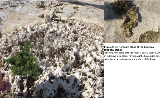
Figure 2-10: Remnant algae at the Loveday Disposal Basin ... 34

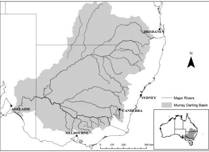
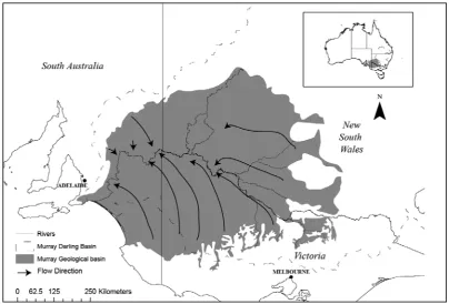
Figure 3-1: The Murray-Darling Basin is a continental drainage basin covering one-seventh of the Australian continent. ... 35

Figure 3-2: Location of study area and field sites. Modified from Lamontagne et. al., (2004). ... 37

Figure 3-3: Berri Evaporation Basin (Image captured from Google Earth®). ... 39

Figure 3-4: The Berri Evaporation Basin: Photograph (Left) of the Berri Evaporation and its proximity to the town of Berri. (Top Right) Oxidised sediments, reduced sulfur and algae in the sediments. (Bottom Right) Reduced sulfur in the sediments immediately below a salt and alga crust. ... 40

Figure 3-5: Aerial photo of the Loveday Disposal Basin and Mussel Lagoon (Image captured from Google Earth®). ... 41

Figure 3-6: The Loveday Disposal Basin: Photograph (Left) of the South Basin in 2010 with dead river red gums. The sediments are oxidised due to exposure to the atmosphere following the experimental reflooding. (Top Right) Standing water near the steam museum and algae growing in the water. (Bottom Right) Sulfide beneath the salt and algae crust at the museum site. ... 42

Figure 3-7: Mussel Lagoon: Photograph (Left) of the Mussel Lagoon which was inundated at the time of sampling in 2010. (Top Right) Algal growth in the water. (Bottom Right) Reduced sulfur beneath the surface sediments. ... 43

Figure 3-8: Total annual rainfall for Loxton (SA) 1897 to 2011. (Data from the Bureau of Meteorology)46 Figure 3-9: Cumulative Residual plot for annual rainfall at Loxton. (Data from the Bureau of Meteorology) ... 47

Figure 3-10: Natural and current river flow downstream of Albury. (Source: MDBA) ... 49

Figure 3-11: Mean daily river height for the Murray River upstream of Lock 3. (Data compiled from http://e-nrims.dwlbc.sa.gov.au/) ... 52

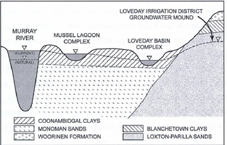
Figure 3-12: The Murray Geological Basin: a small intra-cratonic sedimentary basin within the Murray-Darling Basin. ... 54

(10)

Figure 3-14: Shallow groundwater flow in the Murray Basin. (Modified from Cupper (2006) and Evans

(1988)). ... 58

Figure 3-15: Local Hydrogeology of Mussel Lagoon and Loveday Disposal Basin. (Modified from Lamontagne et al., (2005)). ... 59

Figure 4-1: Location of sampling sites ... 63

Figure 5-1: Electrical Conductivity of 1:5 soil profile of 1:5 soil to water extracts on sediments collected from the Loveday Disposal Basin and Mussel Lagoon. Samples were collected in 2008. ... 72

Figure 5-2: Major anion and cation concentrations from 1:5 soil to water extracts (semi-log plot). Data is from samples collected in 2008. ... 73

Figure 5-3: pH variation with depth for Loveday North and South Basins, the Museum site and Mussel Lagoon on samples collected in 2008 ... 76

Figure 5-4: Chromium-reducible sulfur content of sediments for Loveday North and South, the Museum site and Mussel Lagoon. Data from samples collected in 2008. ... 79

Figure 5-5: Acid-volatile sulfur content of sediments from the Loveday Disposal Basin and Mussel Lagoon. Data from samples collected in 2008. ... 80

Figure 5-6: Total Nitrogen in sediments collected from the Loveday Disposal Basin and Mussel Lagoon. Data from samples collected in 2010. ... 82

Figure 5-7: Total phosphorus concentration in sediments from the Loveday Disposal Basin and Mussel Lagoon. Data collected from samples collected in 2010. ... 83

Figure 5-8: Total carbon concentrations with depth for sediments collected from the Loveday Disposal Basin and Mussel Lagoon. Data collected from collected in 2010. ... 85

Figure 5-9: Chromium-reducible sulfur concentration plotted against time for Loveday North and South (400 and 200 respectively), Mussel Lagoon, and the Berri Evaporation Basin. ... 88

Figure 5-10: Acid-volatile sulfur production with time for Loveday North and South, Mussel Lagoon and the Berri Evaporation Basin ... 89

Figure 5-11: Ferrous iron mobilisation compared with sulfide formation. ... 91

Figure 5-12: Experimental apparatus for sulfide production and iron and phosphate liberation. ... 92

Figure 5-13: Phosphate liberation versus monosulfide production. ... 94

Figure 5-14: Long term phosphate liberation from Mussel Lagoon ... 95

Figure 5-15: Ammonium concentration with time. ... 96

Figure 6-1: Conceptual model for the drying of Mussel Lagoon ... 109

Figure 6-2: Conceptual Model for the inundation of Mussel Lagoon ... 110

Figure 6-3: Conceptual model for the inundation of sediments at the Loveday Disposal Basin and the Berri Evaporation Basin ... 112

(11)

List of Tables

Table 4-1: Analytical methods used for field and experimental samples ... 64

Table 5-1: 1:5 Electrical Conductivity for sediments collected form the Berri Evaporation Basin ... 71

Table 5-2: Electrical Conductivity and pH data for water samples collected. ... 74

Table 5-3: 1:5 soil to water pH data for the Berri Evaporation Basin ... 77

Table 5-4: Chromium-reducible and Acid-volatile sulfur concentrations for sediments collected from the Berri Evaporation Basin in 2010 ... 81

Table 5-5: Total nitrogen and total phosphorus for sediments from the Berri Evaporation Basin. ... 84

Table 5-6: Total Carbon Data for samples from the Berri Evaporation Basin. ... 86

Table 5-7: Rates of chromium-reducible sulfide formation. ... 87

Table 5-8: Rates of acid-volatile sulfide formation. ... 87

Table A-1: Major cation and anion concentrations in sediments... 133

Table A-2: Chromium reducible and Acid Volatile Sulfur ... 134

Table A-3: 1:5 EC and pH ... 135

Table A-4: Sediment Total Phosphorus Concentration ... 138

Table A-5: Sediment total nitrogen and carbon ... 140

Table A-6: Iron and orthophsophate from experimental studies ... 141

Table A-7: CRS and AVS with time from the experimental studies ... 142

Table A-8: Ammonium with time from experimental studies ... 143

Glossary and Terms

Sulfidic Material - A subsoil, waterlogged, mineral or organic material that contains oxidisable sulfur compounds, usually pyrite and iron monosulfide, that has a pH greater than 4 (Isbell, 2002).

(12)

(13)

Chapter 1. Introduction

In recent years, it has become increasingly apparent that water resource management strategies

have had a deleterious effect on inland waterways and floodplain areas in southeastern Australia.

In order to satisfy the economic and political impetus for river navigation, intensive agriculture

and flood mitigation since European settlement, the morphology of surface water networks in

Australia has been changed. New water storage infrastructure aids the extraction and exploitation

of water resources. However, the change to the spatial and temporal availability of water has

removed the natural rhythm of high and low flow periods and imposed a new flow régime, which

for some areas upstream of control structures, has resulted in permanent inundation.

A major environmental issue associated with this river regulation and water resource exploitation

has been the increased salinisation of water and soil resources (Evans and Kellett, 1989). The

management of water levels in rivers, vegetation clearing, coupled with increased water extraction

and irrigation has led to increased recharge of floodplain aquifers (Lamontagne et al., 2004). The

resulting perched water tables have increased water and floodplain salinisation in low-lying

regions within southeastern Australia.

Floodplain and water salinisation is generally equated with salts of sodium and chloride, with

management strategies often based on the physics of solvent and solute movement within

floodplain aquifers. Little attention has been given to the effect that increased salinisation may

have on biogeochemical cycling in inland waterways. Sodium and chloride are known to behave

conservatively in the environment, but other elements such as sulfur, typically encountered as

sulfate (SO42-), have complicated biogeochemical cycles, particularly in sub-aqueous

environments (Lamontagne et al., 2004).

Sulfur undergoes cyclic biotically and abiotically mediated transformations in the environment

(Howarth and Stewart, 1992), which depend on the prevailing redox environment. These changes

in redox environments are brought about through primary production, as oxygen is released

during photosynthesis and consumed by respiration of organic matter (Stumm and Morgan, 1996).

Increased anthropogenic inputs of nutrients, principally nitrogen and phosphorus, from intensive

agriculture and settlement has increased the rate of primary production in inland waterways and

raised the trophic status of these waterways (Cullen, 1986).

Under the low redox potentials found in permanently inundated sub-aqueous environments,

bacteria can utilise sulfate as an oxidant and organic matter as an energy source and reductant

during metabolism. During this anaerobic process, bacteria respire carbon dioxide and reduce

sulfur from its oxidised state (S6+_{) to its reduced state as sulfide (S}2-_{). The reduced sulfur is then}

(14)

mineralised and typically precipitated out of solution following reactions with particulate

inorganic material (Berner, 1970).

Under the anoxic conditions found in permanently inundated waterways, the sulfidic material are

relatively benign (Lamontagne et al., 2004). However, under a higher redox potential, for

example, following exposure to atmospheric oxygen, the sulfide minerals oxidise to liberate

acidity. These issues have been brought to the attention of land managers due to a prolonged and

severe drought experienced in southeastern Australia over the last decade. Reduced rainfall in

much of southeastern Australia during this period saw water levels in inland waterways at their

lowest levels for many decades, which at the same time exposed previously inundated sediments

to the atmosphere (McCarthy et al., 2006).

Under natural conditions, the accumulation of sulfidic material would be abated during the annual

cycle of high and low flows. However, the changes to the hydrological régime brought about

through water resource management strategies have removed this natural cycle of seasonal

changes in redox conditions and have promoted conditions favourable to sulfur reduction in

floodplain wetlands. As a consequence, there has been a continued and unabated accumulation of

environmentally significant quantities of sulfidic material in sub-aqueous sediments in the inland

waterways of southeastern Australia.

The effect on the environment resulting from the oxidation of sulfidic material is well known,

particularly in coastal areas due to acid sulfate soils (ASS) (Dent and Pons, 1995), and mining

through acid mine drainage (AMD) (Drever, 1982). The sulfidic material found in inland

waterways are very recently formed by contemporary bacterial activity (Wallace, 2005), whereas

the sulfide deposits associated with ASS were formed and deposited during the last sea level

maximum, ~10ka, (Sammut and Lines-Kelly, 1996), and the deposits associated with AMD

derived from igneous metal sulfide and coal deposits formed over geological time scales (Drever,

1982; Stumm and Morgan, 1996).

Given the environmental issues associated with ASS and AMD, there has been a great deal of

research domestically and internationally into the oxidative transformation of sulfur in the

environment (Arkesteyn, 1980; Moses et al., 1987; White et al., 1997). Research is also currently

being conducted into the oxidation of sulfidic material in inland areas (Fitzpatrick et al., 2008;

Fitzpatrick et al., 2009). The reductive transformation of sulfur in inland aquatic environments is

well known overseas (Berner, 1970; Berner, 1984), but until recently little research has been

conducted into the reductive transformations of sulfur in inland Australia.

(15)

To guide this research project, the paradigm developed here is that spatial and temporal changes

in water supply have promoted conditions favourable to high rates of bacterial sulfur reduction in

floodplain wetlands in low-lying regions of southeastern Australia.

Building from this paradigm, the aims of this study are to determine the controls and rates of

formation of sulfidic material in floodplain wetlands. The interrelationship between the sulfur

cycle and those of carbon, nitrogen and phosphorus dictates that the cycling of sulfur cannot be

studied in isolation. Hence, a secondary aim is to determine the effect that sulfur cycling can have

on these other cycles.

This research project has been a laboratory based experimental study on the cycling of sulfur in

the sediments of floodplain wetlands. The objectives of this study were to quantify the rates at

which sulfidic material form, the controls on these rates, and to analyse the nutrient pulse from the

sediments under a low redox potential.

Based on their physicochemical properties, their size and location, and previous research, three

wetlands from the Riverland region of South Australia were selected for this study. Two salt

disposal basins, the Berri Evaporation Basin and the Loveday Disposal Basin, were selected to

determine the effect of increased salinity on biogeochemical cycling. Research at the Loveday

Disposal Basin has been ongoing since 2004 and there exists a considerable knowledge base from

which to build. The Berri Evaporation Basin was selected as an analogue to the Loveday Basin to

ascertain if processes at Loveday were representative of wetlands with similar characteristics.

Mussel Lagoon is a freshwater wetland and lies adjacent to the Loveday Disposal Basin and was

selected to provide a comparison of processes in freshwater as opposed to the saline waters and

sediments found in Berri and Loveday (Beavis et al., 2006; Higgins, 2006; Lamontagne et al.,

2004, 2006; Lamontagne et al., 2008; Wallace, 2005; Wallace et al., 2008; Welch et al., 2006;

Welch, 2005).

(16)

Chapter 2. Review of Literature

Introduction

The focus of this research project has been on the biogeochemical cycles of elements in

floodplain wetlands of the lower Murray River. The spatial and temporal changes to the water

cycle in the lower Murray region coupled with intensive agriculture and salinity have altered the

cycling of elements within these wetlands. The effect of water resource management has been a

near permanent water cover in many low-lying floodplain areas, disrupting the biogeochemical

cycles in these waterways (Lamontagne, 2003; Nielsen, 2003).

However, in the last decade, a severe and prolonged drought, together with increasing

over-allocation of water in the Murray-Darling Basin, reduced the water level of many streams and

wetlands, with associated implications for nutrient cycling, and particularly sulfur cycling.

This chapter first describes the anaerobic redox sequence, and then discusses the biogeochemical

cycles of carbon, sulfur, iron, phosphorus and nitrogen. As the research conducted has focused on

the interrelationships between these cycles, there is a deliberate repetition of information.

Wetland Biogeochemistry

Wetlands ecosystems are characterised by soils that are episodically waterlogged, and which often

have high organic matter content (Young, 2001). These episodic periods of waterlogging and

drying control the cycling of nutrients and carbon in floodplain wetland ecosystems (Young,

2001). The most important chemical effect of waterlogging is a reduction in the redox potential

brought about by the degradation of organic matter and microbial metabolism (Manahan, 2005).

When saturated, wetland environments are oxic (enriched in oxygen) at the surface due to

photosynthesis, and anoxic (depleted in oxygen) at depth due to respiration (Giblin and Wieder,

1992). This allows for a spectrum of redox reactions to occur. Redox reactions occur through

electron transfer from one atom to another and are the basis of biogeochemical cycling (Zumdahl,

1997). These electron transfer reactions are kinetically inhibited and proceed more rapidly

through bacterial catalysis in the environment and have the effect of restoring chemical

equilibrium. The measure of a system’s ability to supply electrons is known as the redox

potential, Eh.

Living organisms are thermodynamically unstable and require a continual source of energy to

survive (Reddy and DeLaune, 2008). This energy is initially supplied from the sun;

photosynthesis traps solar energy in chemical bonds as complex organic matter is synthesised

(Reddy and DeLaune, 2008; Stumm and Morgan, 1996). The energy input maintains organisms in

(17)

a state with disequilibrium speciation of carbon, nitrogen, oxygen, phosphorus and sulfur (Stumm

and Morgan, 1996).

To drive the metabolic processes that maintain their disequilibrium steady state, bacteria and other

respiring organisms catalyse redox reactions utilising the organic products of photosynthesis as an

energy source during heterotrophic respiration (Stumm and Morgan, 1996). This energy results

from the electron transfer from the reduced carbon to electron acceptors such as oxygen, nitrate

and sulfate.

Redox Conditions and Processes in

Freshwater Wetlands

The redox conditions and processes in freshwater wetlands are influenced by the cycling of

carbon.

Carbon cycling involves continual synthesis and degradation of organic molecules (Stumm and

Morgan, 1996). Carbon cycling in wetland ecosystems provides the energy required for aquatic

organisms to survive. This energy is obtained directly from the sun through photosynthesis as

organic molecules are synthesised, or transferred through the breakdown of photosynthetic

organisms (Stumm and Morgan, 1996). These two processes, as well as the supply of electron

acceptors exert controls on the redox environments in aquatic ecosystems (Drever, 1982).

2.3.1. Photosynthesis

Carbon fixation during photosynthesis reduces carbon from its oxidised state to a reduced state

(Reddy and DeLaune, 2008). During photosynthesis, autotrophic organisms utilise solar energy to

convert carbon dioxide to organic matter and oxygen, as shown in its simplest form in Equation

2.1 (Drever, 1982):

𝐶𝐶𝑂𝑂2

𝑠𝑠𝑠𝑠𝑠𝑠𝑠𝑠𝑠𝑠𝑠𝑠ℎ𝑡𝑡

�⎯⎯⎯⎯⎯� 𝐶𝐶𝑜𝑜𝑜𝑜𝑠𝑠𝑜𝑜𝑠𝑠𝑠𝑠𝑜𝑜+𝑂𝑂2 (2.1)

This initial gain of energy from the sun and the synthesis of organic molecules is termed primary

production.

However, photosynthesis requires more than just sunlight and carbon dioxide. Autotrophs1_such

as plants require nutrients obtained from nitrogen compounds, phosphorus compounds, and a

1_{Organisms capable of producing complex organic molecules from carbon dioxide during photosynthesis}

5

(18)

range of trace elements. A more complex relationship that includes thesecomponents is given in

Equation 2.2 (Stumm and Morgan, 1996):

In surface waters, these plants are usually microscopic algae, which will grow until the

availability of nutrients is limited, resulting in high concentrations of organic matter (Stumm and

Morgan, 1996). Equation 2.2 also demonstrates the role that phosphorus plays in the rate of

primary production in the aquatic environment. One mole of phosphorus has the potential to result

in the fixation of 106 atoms of carbon and the production of 138 molecules of oxygen and it is

most often the limiting nutrient in primary production in terrestrial ecosystems.

2.3.2. Respiration (Oxygen Reduction)

Photosynthesis promotes higher states of free energy and aquatic organisms that do not source

their energy from photosynthesis, as autotrophs do, source their energy from the breakdown of

organic molecules formed from photosynthesis during heterotrophic2_{respiration (Stumm and}

Morgan, 1996). These reactions are biologically mediated as bacteria obtain a source of energy to

meet their metabolic needs (Drever, 1982).

The decomposition of organic molecules occurs through a succession of energy-yielding reactions

catalysed by organisms at varying trophic (energy) levels (Drever, 1982; Stumm and Morgan,

1996). Given that they source free energy from these decay reactions, bacteria promote and

restore equilibrium by catalysing these reactions and decomposing the unstable products of

photosynthesis (Stumm and Morgan, 1996).

As the microbially mediated redox reactions involve energy gains by bacteria, preference will be

given to those electron acceptors that yield the most energy, and occur in an order which can be

predicted from thermodynamics (Stumm and Morgan, 1996). The result of this preferential

selection of electron acceptors is a sequence of reactions and zoning of redox processes as the

supply of electron acceptors is exhausted (Stumm and Morgan, 1996).

These redox reactions occur at successively lower Eh levels and involve the oxidation of organic

matter and the reduction of an oxidant. A progression of respiration reactions generate

progressively lower energy yields which also serve to reduce organic matter (Drever, 1982;

Howarth and Stewart, 1992).

2_{Organisms incapable of fixing carbon dioxide and requiring organic carbon as an energy source for}

synthesis

106CO2 + 16NO3- + HPO42- + 122H2O + 18H+→[(CH2O)₁₀₆(NH3)₁₆(H3PO4)] + 138O2 (2.2)

6

(19)

At the highest energy level, the succession begins with oxygen, shown in Equation 2.3, which is

the reverse of photosynthesis (Equation 2.2).

[(CH2O)₁₀₆(NH3)₁₆(H3PO4)] + 138O2→106CO2 + 16NO3- + HPO42- + 122H2O + 18H+ (2.3)

Equations 2.2 and 2.3 together maintain a steady state between the rate of photosynthetic

production and respiration, or net primary productivity (Stumm and Morgan, 1996). The chain

length of the organic matter is reduced as organic matter decomposes during respiration. In

addition, stoichiometric liberation of carbon dioxide, nitrate and phosphate occurs (Redfield,

1934; Redfield, 1958).

2.3.3. Ecological Redox Sequence

The result of photosynthesis and respiration in waterways is redox stratification, with a high Eh

(redox potential) near the surf ace where photosynthesis is occurring, and a lower Eh where

respiration is occurring, effectively forming a redox cline between oxic and anoxic conditions in

the water column (Holmer and Storkholm, 2001).

The accumulation of organic matter from photosynthesis in aquatic ecosystems is typically much

greater than the rate of aerobic respiration, ultimately resulting in the complete exhaustion of

oxygen and zones where other electron acceptors are utilised during anaerobic respiration.

Where free oxygen has been completely consumed and anoxia is induced, the respiration and

decay of unstable organic matter continues through a series of energy yielding redox reactions

(Drever, 1982; Stumm and Morgan, 1996). These anaerobic decay reactions are bacterially

mediated by lithotrophs3_{and have the effect of consuming acidity and mineralising carbon to}

either carbon dioxide or carbonate. Given the gains in free energy by bacteria, competition exists

between bacteria for energy sources. As a result, zones form in soil and water columns where

bacteria utilising other electron acceptors are excluded. The predominant ecological anaerobic

redox sequence predicted from thermodynamics is shown in Figure 2-1.

3_{Organisms which utilise inorganic compounds as an electron acceptor during synthesis}

7

(20)

[image:20.595.140.443.67.497.2]

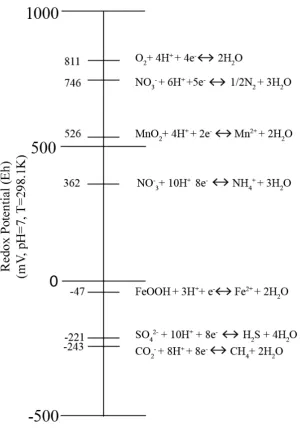
Figure 2-1: Ecological Redox Sequence(Data from Stumm and Morgan (1996)).

The ecological redox sequence begins with aerobic respiration and reduction of oxygen at

the highest redox potential. Anaerobic respiration proceeds beginning with nitrate as an

oxidant followed by manganese oxide.

At significantly lower redox potentials, iron reduction can proceed followed by sulfate

reduction and methanogenesis proceed under strictly anoxic conditions.

Following the reduction of oxygen during aerobic respiration, the ecological redox sequence

proceeds anaerobically with denitrification, manganese reduction, iron reduction, sulfate

reduction and methanogenesis, with fermentation reaction occurring at various redox potentials

(Reddy and DeLaune, 2008; Schlesinger, 1997).

(21)

2.3.4. Denitrification

Following the reduction of oxygen during aerobic respiration, the sequence of anaerobic redox

reactions continues: nitrate as an oxidant leads to the formation of nitrogen gas in denitrification

as shown in Equation 2.4. Denitrification occurs through a series of intermediate reactions

forming metastable intermediates as shown in Equation 2.5 (Appelo and Postma, 2007; Drever,

1982):

5𝐶𝐶𝑜𝑜𝑜𝑜𝑠𝑠𝑜𝑜𝑠𝑠𝑠𝑠𝑜𝑜 + 4𝑁𝑁𝑂𝑂3− + 4𝐻𝐻+→2𝑁𝑁2 + 5𝐶𝐶𝑂𝑂2 + 2𝐻𝐻2𝑂𝑂 (2.4)

𝑁𝑁𝑂𝑂3−(𝑜𝑜𝑎𝑎)→ 𝑁𝑁𝑂𝑂2−(𝑜𝑜𝑎𝑎)→ 𝑁𝑁𝑂𝑂(𝑒𝑒𝑠𝑠𝑒𝑒𝑒𝑒𝑒𝑒𝑒𝑒𝑜𝑜𝑜𝑜𝑒𝑒𝑐𝑐𝑠𝑠𝑒𝑒𝑙𝑙)→ 𝑁𝑁2𝑂𝑂(𝑠𝑠𝑜𝑜𝑠𝑠)→ 𝑁𝑁2(𝑠𝑠𝑜𝑜𝑠𝑠) (2.5)

The reduction of nitrate results in the formation of molecular nitrogen, a gas which has the diatomic molecular structure N≡N with a triple bond. The strong bonding that exists means that nitrogen gas is very unreactive, or inert. Denitrification can therefore be important in controlling

the nutrient balance of aquatic ecosystems (Stumm and Morgan, 1996).

2.3.5. Manganese and Iron Reduction

In wetland sediments, Fe(III) and Mn(IV) can be reduced by microorganisms or strong reducing

agents to Fe(II) and Mn(II) (Reddy and DeLaune, 2008). The oxidised forms of iron and

manganese are typically insoluble amorphous or crystalline forms, Fe(OH)3, FeOOH, and MnO2.

Manganese reduction proceeds where the supply of nitrate has been exhausted and occurs at a

higher redox potential than iron reduction. Manganese reduction results in the liberation of

soluble manganese as Mn2+ _{as shown in Equation 2.6:}

2𝑀𝑀𝑀𝑀𝑂𝑂2+𝐶𝐶𝑜𝑜𝑜𝑜𝑠𝑠𝑜𝑜𝑠𝑠𝑠𝑠𝑜𝑜+ 3𝐻𝐻+→2𝑀𝑀𝑀𝑀2++𝐻𝐻𝐶𝐶𝑂𝑂3−+𝐻𝐻2𝑂𝑂 (2.6)

Iron reduction occurs at a considerably lower redox potential than manganese reduction. During

iron reduction, oxidised iron minerals are reduced with the liberation of Fe2+_{as shown in Equation}

2.7:

4𝐹𝐹𝐹𝐹𝑂𝑂𝑂𝑂𝐻𝐻+ 7𝐻𝐻+₊_𝐶𝐶

𝑜𝑜𝑜𝑜𝑠𝑠𝑜𝑜𝑠𝑠𝑠𝑠𝑜𝑜+𝐻𝐻2𝑂𝑂 →4𝐹𝐹𝐹𝐹2++𝐻𝐻𝐶𝐶𝑂𝑂3−+ 6𝐻𝐻2𝑂𝑂 (2.7)

(22)

The reduction of iron and manganese can occur abiotically through a simple redox reaction with

organic matter, and this was long believed to be the only mechanism. However, the reaction can

also be mediated by bacteria provided they are in contact with the mineral surface (Lovley, 1991).

Biologically mediated processes are responsible for most of the soluble iron and manganese in

aquatic ecosystems and are intrinsically tied to the cycling of sulfur and phosphorus. Iron and

manganese oxides have high adsorption capacities with a high affinity for trace elements and

oxyanions that can be sorbed to the surface. This has the effect of regulating the concentrations of

these elements in aquatic ecosystems (Appelo and Postma, 2007; Drever, 1982; Lovley, 1991;

Raiswell and Canfield, 2012). Therefore, the dissolution of these manganese and iron minerals

under low redox potentials results in the liberation of not only soluble manganese and iron, but

the trace elements and oxyanions that were sorbed to the surfaces of these minerals (Drever,

1982).

2.3.6. Nitrate Ammonification

Nitrate can be reduced to ammonium during anaerobic metabolism; this occurs at Eh values lower

than manganese reduction, but higher than iron reduction (Stumm and Morgan, 1996). The

process can be assimilatory and dissimilatory as nitrate is reduced to ammonium. The

assimilatory pathway occurs when nitrate is reduced to ammonium which is subsequently utilised

to synthesise new cells (Page et al., 2003) (Equation 2.8). The dissimilatory pathway involves

bacterial reduction of nitrate to ammonium, which is not incorporated into cell structures but goes

into solution (Page et al., 2003).

𝑁𝑁𝑂𝑂3−+ 2𝐶𝐶𝑜𝑜𝑜𝑜𝑠𝑠+ 2𝐻𝐻2𝑂𝑂+ 2𝐻𝐻+→ 𝑁𝑁𝐻𝐻4++ 2𝐶𝐶𝑂𝑂2+𝐻𝐻2𝑂𝑂 (2.8)

2.3.7. Fermentation

Fermentation reactions, shown in Equation 2.9, can occur at various Eh values and involve the

breakdown of complex organic compounds to organic acids and alcohols and then further to

methane during methanogenesis, which occurs at a lower Eh (Stumm and Morgan, 1996).

The short-chain volatile fatty acids (for example, formate and acetate) are more labile than

longer-chained fatty acids, and are ultimately the energy source for the anaerobic reactions involving

bacteria, particularly the iron- and sulfate-reducing and methanogenic bacteria. As these reactions

provide the energy sources for anaerobic metabolism, where carbon concentrations are low, the

rate at which the fermentation reactions proceed can influence the rates other reactions

particularly in polluted waterways.

(23)

H2 + CO2 → CH4

Complex organic material → Organic acids

CH3COO-→ CH4

(2.9)

(Stumm and Morgan, 1996)

2.3.8. Sulfate Reduction

Sulfate reducing bacteria occupy a redox niche at higher Eh than that of methanogenic bacteria.

They require the fermentation products during metabolism (Winfrey, 1983) when they utilise

sulfate as a terminal electron acceptor and organic carbon as an energy source, as shown in

Equation (2.10):

𝑆𝑆𝑂𝑂42− + 2𝐶𝐶𝑜𝑜𝑜𝑜𝑠𝑠𝑜𝑜𝑠𝑠𝑠𝑠𝑜𝑜 + 2𝐻𝐻2𝑂𝑂 → 𝐻𝐻2𝑆𝑆 + 2𝐻𝐻𝐶𝐶𝑂𝑂3− (2.10)

In anoxic sediments, sulfate reduction can be the dominant source of carbon mineralisation,

provided there is a ready supply of organic carbon and sulfate (Berner, 1970, 1982, 1985; Holmer

and Storkholm, 2001).

Sulfate reduction produces hydrogen sulfide, which is highly toxic to most aquatic organisms and

has a characteristic odour that can also impact on the aesthetics of an ecosystem (Drever, 1982;

Lamontagne, 2003; Lamontagne et al., 2004). Sulfide is also a powerful reducing agent and can

convert iron (III) in oxides oxy(hydr)oxides to iron (II) in sulfides, altering the colour of

sediments from red to black, as well as liberating species such as phosphate and trace metals, that

were sorbed to the surface of the iron oxides (Drever, 1982). It is these effects that are being

investigated in this research project.

2.3.9. Methanogenesis

Methanogenesis is intimately tied to the processes of fermentation. The short-chained volatile

fatty acids and carbon dioxide formed during fermentation are reduced to methane shown in

Equation 2.11:

Methanogenesis occurs at a lower redox potential than sulfate reduction and is the terminal step in

the decay of organic molecules (Stumm and Morgan, 1996).

𝐶𝐶𝑂𝑂2+𝐻𝐻2→ 𝐶𝐶𝐻𝐻4+ 2𝐻𝐻2𝑂𝑂 (2.11)

(24)

Similar to sulfate reducing bacteria, methanogens can only utilise certain organic molecules as

energy sources during metabolism, including acetate and hydrogen gas. Sulfate reducers are more

efficient at utilising these organic molecules and outcompete methanogens even at freshwater

sulfate concentrations (Lovley and Klug, 1983). Typically, sulfate concentrations in most waters

are low, which results in methanogenesis occurring in a zone almost directly underlying the zone

of sulfate reduction (Schlesinger, 1997).

Biogeochemical Cycling

Biogeochemical cycling refers broadly to the cycling of matter, particularly nutrients, through an

ecosystem (Manahan, 2005; Reddy and DeLaune, 2008). The above mentioned anaerobic redox

sequence plays a major role in these cycles, particularly nutrient cycling, in wetland ecosystems.

The biogeochemical cycling of these elements also involves oxidative transformations as well as

the already mentioned reductive transformations.

The energy trapped from the sun during photosynthesis also requires phosphorus and nitrogen, as

well as other trace elements to proceed. As noted earlier, the supply of these nutrients can limit

the rate of primary productivity in aquatic ecosystems, but the movements of these elements

through a system are interconnected with one another. The focus of this research is sulfur cycling

with a particular focus on the reduction of sulfur by bacteria and the effect that this has on other

biogeochemical cycles. However, the cycling of sulfur is interdependent of the cycling of carbon,

nitrogen, phosphorus and iron, and therefore sulfur cannot be studied in isolation. These other

cycles will be described in later sections.

2.4.1. Sulfur Cycling

In most freshwater systems sulfur cycling plays a modest role in biogeochemical functioning and

carbon mineralisation. However, sulfur concentrations in most ecosystems have increased due to

anthropogenic pollution such as acid rain and the increased exploitation of groundwater resources

(Holmer and Storkholm, 2001). Interest has also been piqued as the trophic status of many

waterways has changed from oligotrophic and mesotrophic to eutrophic4_{due to the effect of}

sulfur cycling on the binding capacity of iron (oxyhydr)oxides and phosphorus retention (Holmer

and Storkholm, 2001). Sulfur cycling is also important due to the oxidative transformations of

sulfur under oxic conditions involving iron.

Sulfur occurs in the Earth’s crust with an abundance of 0.047% and is widely distributed in both

4_{The trophic state is a measure of the productivity of a waterway. Waterways are classed as oligotrophic}

(low productivity), mesotrophic (moderate productivity) and eutrophic (high productivity) 12

(25)

free and combined forms (Grinenko and Ivanov, 1983). Sulfur undergoes cyclic transformations

in the environment, controlled by the prevailing redox environment, and can exist in oxidation

states from -2 (sulfide) to +6 (sulfate) (Grinenko and Ivanov, 1983).

The most oxidised form of sulfur, sulfate, is the form of sulfur typically encountered in the

surficial environment. Most sulfates are soluble, and occur as minerals only in evaporite deposits,

but a few are insoluble, including calcium, strontium, lead and barium sulfates (Grinenko and

Ivanov, 1983). The most abundant of the poorly soluble sulfates are gypsum (CaSO4·2H2O) and

anhydrite (CaSO4). Removal of sulfur from the cycle occurs when these minerals are precipitated,

and deposits of gypsum and anhydrite comprise the biggest sink of sulfur (Grinenko and Ivanov,

1983).

Sulfide, the most reduced form of sulfur, occurs in aqueous solutions and has different chemical

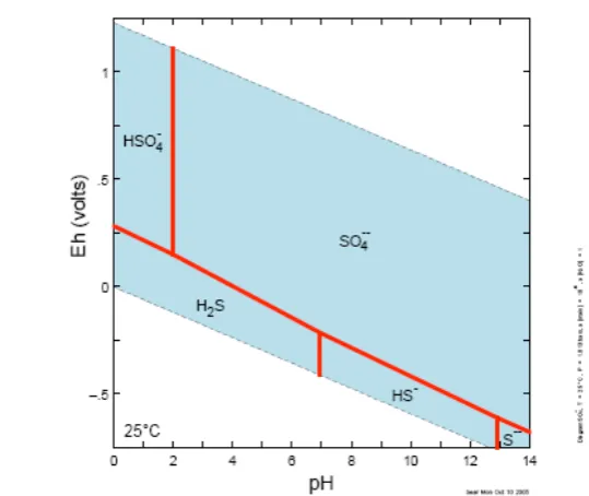
and geochemical properties compared to sulfate. Figure 2-2 shows the predominant sulfur species

at equilibrium under standard temperature and pressure (298 K and 1 atm.). Sulfide species are

dominant only under low redox potentials (or anoxic conditions) at all pH values. Most sulfides,

with the exception of those of the alkali metals and alkaline earths, form insoluble mineral

species, but when anoxic conditions change to oxic, the sulfides are oxidised to form soluble and

transient sulfates (Brimblecombe, 2005; Goldhaber, 2005). When sulfate is exposed to anoxic

conditions, the opposite occurs and the sulfate is reduced to insoluble sulfide, which results in the

sequestration of metals and sulfur. However, whilst the reduction of sulfate to sulfide is

spontaneous and thermodynamically favoured under standard temperature and pressure, the

reaction is kinetically inhibited (Grinenko and Ivanov, 1983).

The reduction of sulfate is catalysed by bacteria during their metabolism and is termed bacterial

sulfate reduction. The cycling of sulfur in a wetland is shown diagrammatically in Figure 2-3.

During microbial metabolism, sulfate is utilised as a terminal electron acceptor. The result of this

is a change in oxidation state of sulfur from +6 to -2 and the formation of oxidised carbon, usually

as bicarbonate, HCO3-. Sulfide, which is a by-product of this metabolism, subsequently reacts

with particulate iron minerals to form sulfide minerals such as pyrite (FeS2) (Berner, 1970).

(26)

Figure 2-2: Equilibrium distribution of sulfur species in water at 298K, 1 atm, and [S] =10-6_{(Diagram generated using the Geochemist’s Workbench®).}

The Pourbaix diagram shows the prevalence of oxidised and reduced sulfur as a function of redox potential and pH. Sulfate predominates at higher redox potential and sulfide at low redox potentials.

[image:26.595.141.411.73.300.2]

Bacterial sulfate reduction occurs under anoxic conditions and the importance of sulfate reduction Figure 2-3: Sulfur Cycle. (Modified from Holmer and Storkholm (2001)).

Sulfur undergoes cyclic transformations in the environment depending on the prevailing redox conditions. The reduction of sulfate to sulfide is biologically mediated by bacteria and occurs in anoxic conditions. The oxidation of sulfide to sulfate is both abiotic and biotic.

(27)

in wetland biogeochemistry depends on the presence of labile organic matter and the supply of

sulfate as shown in Equation 2.12 (Berner, 1970):

𝑆𝑆𝑂𝑂42− + 2𝐶𝐶𝑜𝑜𝑜𝑜𝑠𝑠𝑜𝑜𝑠𝑠𝑠𝑠𝑜𝑜 + 2𝐻𝐻2𝑂𝑂 → 𝐻𝐻2𝑆𝑆 + 2𝐻𝐻𝐶𝐶𝑂𝑂3− (2.12)

Energy sources for sulfate reduction are typically fermentation products, usually hydrogen gas

and short chained volatile fatty acids ranging from formate up to benzoate (Holmer and

Storkholm, 2001; Lovley and Klug, 1986; Postgate, 1979; Smith, 1981). The concentration of

either labile organic carbon or sulfate can limit the rate of sulfate reduction. Berner (1984), gave a

sulfate concentration of 5 mM where the rate of sulfate reduction is independent of the sulfate

concentration and is limited by the labile organic carbon concentration in marine ecosystems.

The species of sulfide formed is controlled by the pH of the solution, and total sulfide (or H2S in

equations such as those above) should be taken to represent the sum of H2S, HS-, and S2- with pKa

values shown below (I.U.P.A.C., 1969):

𝐻𝐻2𝑆𝑆 ↔ 𝐻𝐻𝑆𝑆−+𝐻𝐻+ pKa = 7.04

𝐻𝐻𝑆𝑆−_{↔ 𝑆𝑆}2−₊_𝐻𝐻+ _pK_a_{= 12.88}

Hydrogen sulfide, H2S, is a gas at standard temperature and pressure; it contributes in part to the

noxious odours associated with sulfide deposits and is toxic to aquatic organisms (Holmer and

Storkholm, 2001). Sulfide is a powerful reducing agent. However, as noted above, it reacts with

detrital minerals to form insoluble metal sulfides. By reacting with these minerals, the sulfide is

sequestered in the sediments of wetlands, and the toxicity is minimised as these sulfide minerals

are formed (Appelo and Postma, 2007). Sediments and soils that contain appreciable quantities of

sulfide minerals are termed sulfidic material (Isbell, 2002).

Sulfate reduction is often used in bioremediation, particularly in acidic environments. Inducing

anoxia in acidic environments and promoting bacterial sulfate reduction, usually by organic

matter, helps to neutralise acidity since H2S is a much weaker acid than H2SO4,and bacterial

sulfate reduction generates inorganic carbon (Johnson and Hallberg, 2005).

Formation of Sulfidic Material

In natural surficial environments, the formation of sulfidic material begins with bacterial sulfate

reduction. The reduced sulfur formed during this process reacts with dissolved iron (and other

cations) to form sulfide minerals, initially forming iron monosulfide as shown in Equation 2.13:

𝐹𝐹𝐹𝐹2+₊_𝐻𝐻

2𝑆𝑆 → 𝐹𝐹𝐹𝐹𝑆𝑆+ 2𝐻𝐻+ (2.13)

The monosulfide formed in Equation 2.13 is a metastable intermediate and has been difficult to

(28)

characterise given its reactivity and the rate at which it oxidises on exposure to air (Pyzik and

Sommer, 1981). Iron monosulfide stains sediments black and is commonly referred to as

monosulfidic black ooze (MBO) or acid volatile sulfide (AVS), as it readily dissolves in

hydrochloric acid to form hydrogen sulfide (Bush et al., 2004). A more stable sedimentary sulfide

mineral is pyrite, which forms through an oxidation reaction with H2S as shown in Equation 2.14

(Schoonen, 2004):

𝐹𝐹𝐹𝐹𝑆𝑆+𝐻𝐻2𝑆𝑆 → 𝐹𝐹𝐹𝐹𝑆𝑆2+𝐻𝐻2 (2.14)

As well as the reaction of FeS with elemental sulfur (Berner, 1984):

𝐹𝐹𝐹𝐹𝑆𝑆+𝑆𝑆0_{→ 𝐹𝐹𝐹𝐹𝑆𝑆}

2 (2.15)

The elemental sulfur in Equation 2.15 is a product of anaerobic oxidation, where reduced sulfur,

H2S or bisulfide HS-, is oxidised to elemental sulfur, S0, by Iron (III), Manganese (IV) or another

metal ion .

The oxidation of reduced sulfur to elemental sulfur by iron (II) is shown in Equation 2.16 (Lovley

and Phillips, 1994; Steudel, 1996):

𝐻𝐻2𝑆𝑆+ 2𝐹𝐹𝐹𝐹3+→ 𝑆𝑆0+ 2𝐻𝐻++ 2𝐹𝐹𝐹𝐹2+ (2.16)

Whilst represented in Equation 2.16 as S0_{, the reaction is thought to proceed through a}

polysulfide, which is a mix of both S0_{and S(-II), with the sulfur in pyrite being} 2−

2

S

, which is a mix of both S2- _{and S}0_{(Rickard, 2012). Equation 2.15 can be written as (Rickard, 2012):}

𝐹𝐹𝐹𝐹𝑆𝑆+𝑆𝑆𝑠𝑠(−𝐼𝐼𝐼𝐼)→ 𝐹𝐹𝐹𝐹𝑆𝑆2+𝑆𝑆(𝑠𝑠−1)(−𝐼𝐼𝐼𝐼) (2.17)

As noted earlier, hydrogen sulfide is toxic to aquatic organisms, however, the reaction with iron

limits this toxicity, since the formation of metal sulfides limits the concentration of dissolved

sulfide as well as sequestering heavy metals in wetland sediment (Megonigal et al., 2005). If the

concentration of H2S is very high for a prolonged period of time, then the formation of sulfide

minerals can be limited by the presence of detrital iron minerals (Berner, 1970).

Sulfide Oxidation

Pyrite is stable at a low Eh and remains benign unless exposed to oxidising conditions, where it

oxidises to form sulfuric acid. The overall reaction is shown in Equation 2.18 (Appelo and

Postma, 2007):

𝐹𝐹𝐹𝐹𝑆𝑆2+7₂𝑂𝑂2+𝐻𝐻2𝑂𝑂 → 𝐹𝐹𝐹𝐹2++ 2𝑆𝑆𝑂𝑂42−+ 2𝐻𝐻+ (2.18)

(29)

Pyrite oxidation to sulfate by oxygen releases ferrous iron and acidity. Furthermore the ferrous

iron produced from the initial oxidation of pyrite with oxygen can be further oxidised by oxygen

shown in Equation 2.19:

𝐹𝐹𝐹𝐹2+_{+ 1 4}_{� 𝑂𝑂}

2+𝐻𝐻+→ 𝐹𝐹𝐹𝐹3++ 1 2� 𝐻𝐻2𝑂𝑂 (2.19)

Unless the pH is extremely low, the ferric iron formed is hydrolysed to form a precipitate of

ferrihydrite shown in Equation 2.20 (Watts and Teel, 2005):

𝐹𝐹𝐹𝐹3+_{+ 3}_𝐻𝐻

2𝑂𝑂 → 𝐹𝐹𝐹𝐹(𝑂𝑂𝐻𝐻)3+ 3𝐻𝐻+ (2.20)

If the pH is below ~4, Equation 2.19 can be catalysed by bacteria, sp. Acidithiobacillus

ferrooxidans and can increase the rate of oxidation by several orders of magnitude (Appelo and

Postma, 2007). The ferric iron produced can also be reduced by pyrite, shown in Equation 2.21,

and sulfide is again oxidised.

𝐹𝐹𝐹𝐹𝑆𝑆2+ 14𝐹𝐹𝐹𝐹3++ 8𝐻𝐻2𝑂𝑂 →15𝐹𝐹𝐹𝐹2++ 2𝑆𝑆𝑂𝑂42−+ 16𝐻𝐻+ (2.21)

The reduction of iron by pyrite produces significantly more acidity than the abiotic reactions

involving atmospheric oxygen and generates significantly more acidity (Moses and Herman,

1991; Moses et al., 1987; Singer and Stumm, 1970). The ferrous iron produced from the oxidation

of pyrite is oxidised via Equation 2.19, providing a fast autocatalytic mechanism for the

generation of significant quantities of acidity which can occur in the absence of dissolved oxygen

(Bierens de Haan, 1991; Moses et al., 1987; Nordstrom, 1982; Somerville et al., 2004).

The oxidation of sulfides in sulfidic material does not necessarily mean that sediments and soils

will become sulfuric material. The formation of these minerals generates alkalinity through the

mineralisation of organic carbon to carbonate during anaerobic metabolism, which in many

instances provides ample buffering capacity to offset the acidity generated during oxidation.

However, this depends on the hydrologic régime and the degree of openness of the system as

alkalinity can be exported form the system.

The oxidation of sulfide minerals in the environment is well documented, given the deleterious

effects of the low pH associated with the generation of acidity. Sulfide minerals are frequently

encountered in mineral deposits including sulfide ore bodies and coal deposits, the exploitation of

which can lead to acid mine drainage (Blowes et al., 2005). Sulfide minerals are also often

encountered in coastal areas, where Holocene age deposits of these minerals were laid down

during the last sea level rise. The soils that have developed from these marine sediments through

(30)

pedogenic processes are common in low-energy tidal environments. It is now evident most of

Australia’s coastal lowland areas are underlain with sulfidic material and sulfide-rich sediments

(Dent, 1986; White et al., 1997). Often, the management strategy employed to mitigate the

oxidation of sulfidic material is to inundate the soils and sediments with water to induce anoxia

and halt oxidation (Simpson, 2008; White et al., 1997).

2.4.2. Iron Cycling

The cycling of sulfur in the aquatic environment is intrinsically tied into the cycling of iron

(Raiswell and Canfield, 2012). The oxidation and reduction of iron in wetlands mediates the

concentrations of many other elements. The interaction of iron in the environment with other

elements can be grouped into abiotic and biotic processes (Raiswell and Canfield, 2012).

The hydrated ferric oxides formed through the oxidation of ferrous iron have a surface charge,

and therefore ions in solution will sorb onto these surfaces (Appelo and Postma, 2007; Stumm and

Morgan, 1981). This surface charge is highly variable and is governed by protonation and

deprotonation reactions or the acid-base behaviour of the surface hydroxyl groups, meaning that

the surface charge is pH dependent. The protonation and deprotonation reactions of goethite are

given in Equation 2.22 as an example (Stumm and Morgan, 1996) :

≡FeOH2+ ↔ ≡FeOH + H+↔ ≡FeO- + H+ (2.22)

Most oxides, oxyhydroxides and hydroxides of aluminium and iron possess this amphoteric

behaviour, with the surface charge being positive at low pH values and negative at high pH values

(Stumm and Morgan, 1996). The importance of this surface charge comes from the ability of

oxyanions to adsorb onto these surfaces (Stumm and Morgan, 1996). The variable charge allows

these solids to sorb ions from solution without exchanging other ions in equivalent proportion as

is the case with ion exchange (Stumm and Morgan, 1996). This is significant in wetland

ecosystems with both oxic and anoxic conditions, because it exerts controls on the cycling of

phosphorus. A more detailed description of phosphorus cycling is provided below, however, it

should be noted here that phosphorus, encountered as the oxyanion orthophosphate PO43-, sorbs

very strongly to the iron (oxyhydr)oxides and becomes sequestered and occluded in sediments

(Stumm and Morgan, 1996). This is significant for biogeochemical cycling in these environments,

because the iron (oxyhydr)oxides are soluble under the low Eh in the anoxic environments of

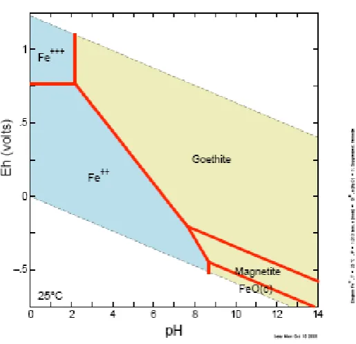
permanently inundated and waterlogged soils and sediments. The Pourbaix diagram for iron at

298K and 1 atm. shown in Figure 2-4 highlights the instability of iron at low Eh and acidic pH

values.

The reduction of iron (oxyhydr)oxides can be an abiotic reaction, particularly in the presence a

(31)

Baldwin, 2007; Canfield et al., 1993).

𝐻𝐻2𝑆𝑆+𝐹𝐹𝐹𝐹𝑂𝑂𝑂𝑂𝐻𝐻+ 4𝐻𝐻+→ 𝑆𝑆0+ 2𝐹𝐹𝐹𝐹2++𝐻𝐻2𝑂𝑂 (2.23)

In addition, the reduction of iron (oxyhydr)oxides can also be microbially mediated as shown in

Equation 2.24 (Lovley, 1991):

4𝐹𝐹𝐹𝐹𝑂𝑂𝑂𝑂𝐻𝐻+ 7𝐻𝐻+₊_𝐶𝐶

𝑜𝑜𝑜𝑜𝑠𝑠𝑜𝑜𝑠𝑠𝑠𝑠𝑜𝑜 →4𝐹𝐹𝐹𝐹2++𝐻𝐻𝐶𝐶𝑂𝑂3−+ 5𝐻𝐻2𝑂𝑂 (2.24)

The biologically mediated reduction of iron (oxyhydr)oxides is an important process in the

mineralisation of organic matter in wetland ecosystems and supplements abiotic dissolution

(Gachter, 2003). Iron reduction and the liberation of ferrous iron ultimately provides a buffer

against increasing dissolved sulfide concentrations as the ferrous iron ultimately forms iron

sulfide, (both pyrite and monosulfides) as well as buffering the concentrations of trace metals

sorbed to the surface of the iron (oxyhydr)oxides (Poulton et al., 2004).

The reduced iron produced from iron reduction of sulfide oxidation is reoxidised at the

anoxic-oxic boundary, and iron (oxyhydr)oxides may represent a significant component of the settling

particles (Singer and Stumm, 1970); this is shown diagrammatically in Figure 2-5.

This process effectively forms a redox buffer that limits the spread of pollutants which are

generally more soluble under oxidising conditions (Stumm and Morgan, 1996)

(32)

Figure 2-4: Equilibrium Diagram for Iron at 298K, 1 atm. and [Fe] = 10-6_.

(Diagram generated with the Geochemist’s Workbench®)

[image:32.595.160.418.75.324.2]

The Pourbaix diagram for iron shows that the dominant form of iron at neutral pH and higher redox potentials is as goethite; ferrihydrite can also occur metastably. Under lower redox potentials, goethite is unstable and dissolves to liberate ferrous iron (Fe2+_).

Figure 2-5: Iron Cycle

The cycling of iron in wetland sediment’s involves the reductive and oxidative transformation of iron between oxidation states, Fe3+ _↔Fe2+_{. Coincident with these processes are the}

liberation of trace metals and phosphate under reducing conditions, but the sorption of these elements to Fe (oxyhdr)oxides under oxidising conditions, effectively forming a ‘redox’ buffer for the transport of these species.

(33)

The Pourbaix diagram for the Fe-S system (Figure 2-6) shows the predominant iron and sulfur

species at 298 K and 1 atm.. The predominant species is goethite for high pH and Eh, but

reduced aqueous ferrous iron at the lower pH and Eh. The stability field for pyrite is narrow,

around circum-neutral pH and low Eh.

Figure 2-6: Equilibrium diagram for the Fe-S system at 298K and 1 atm. ([Fe] and [S] = 10-6_{) (Diagram generated using the Geochemist’s Workbench®).}

The Pourbaix diagram for the Fe-S system showing predominant dissolved species and stable solid phases. Goethite is the most predominant mineral phase at high redox potentials, while pyrite and troilite (non-stoichiometric pyrrhotite Fe1-XS) occur at lower redox potentials and

magnetite at higher pH values.

2.4.3. Phosphorus cycling

Phosphorus is an essential macronutrient and is often the limiting nutrient in primary productivity,

particularly in freshwater ecosystems (Stumm and Morgan, 1996). Phosphorus is ultimately

sourced from phosphate minerals in weathered rocks and atmospheric inputs such as soil particles,

pollen, and the particulates associated with the burning of coal, oil and plants (Berner and Berner,

1996).

Phosphorus is an essential nutrient in the production of organic matter, and the amount of

phosphorus sourced from weathered rocks is considerably less than that incorporated into organic

matter. The deficit is made up from the recycling of biological material as noted above (Berner

and Berner, 1996). There is a biological conservation of phosphorus, so the phosphorus released

through the respiration of organic matter tends to be rapidly cycled back into organic matter

(Berner and Berner, 1996).

(34)

Due to phosphorus being sourced principally from weathering, it is mainly in an insoluble form as

the calcium phosphate, apatite Ca5(PO4)3(F, Cl, OH). If released as soluble phosphate, it is

quickly sorbed into soil and sediments by iron, aluminium, calcium or clay minerals to produce

biologically inaccessible insoluble forms (Berner and Berner, 1996). This inaccessibility of

phosphorus in aquatic environments means it is often a limiting nutrient in primary productivity

(Berner and Berner, 1996).

Unlike other elements, the biogeochemistry of phosphorus does not entail changes in redox state

or a stable gaseous phase, but protonation and deprotonation reactions occur, as shown below in

Equations 2.25, 2.26, and 2.27 (Stumm and Morgan, 1996):

𝐻𝐻3𝑃𝑃𝑂𝑂4↔ 𝐻𝐻2𝑃𝑃𝑂𝑂4−+𝐻𝐻+ pKa1 = 2.1 (2.25)

𝐻𝐻2𝑃𝑃𝑂𝑂4−↔ 𝐻𝐻𝑃𝑃𝑂𝑂42−+𝐻𝐻+ pKa2 = 7.2 (2.26)

𝐻𝐻𝑃𝑃𝑂𝑂42−↔ 𝑃𝑃𝑂𝑂43−+𝐻𝐻+ pKa3 = 12.3 (2.27)

At near-neutral pH, the dominant species encountered is HPO42-

Whilst phosphorus does not undergo cycling transformations between different oxidation states,

the supply of phosphate to an ecosystem, particularly an aquatic ecosystem, can be controlled by

redox conditions. Iron (oxyhydr)oxides will sorb phosphorus as orthophosphate, although

eventually, macroscopic phosphate minerals can form, such as vivianite (Fe2+

3(PO4)2·8H2O) and

strengite (Fe3+_PO

4·2H2O) as shown in Equations 2.28, 2.29 and 2.30:

𝐹𝐹𝐹𝐹3+₊_𝐹𝐹−_{↔ 𝐹𝐹𝐹𝐹}2+_→₃_{𝐹𝐹𝐹𝐹}2+_{+ 2}_{𝐻𝐻𝑃𝑃𝑂𝑂}

42−+ 8𝐻𝐻2𝑂𝑂 → 𝐹𝐹𝐹𝐹3𝐼𝐼𝐼𝐼(𝑃𝑃𝑂𝑂4)2∙8𝐻𝐻2𝑂𝑂+ 2𝐻𝐻+ (2.28)

𝐹𝐹𝐹𝐹(𝑂𝑂𝐻𝐻)3(𝑆𝑆)+𝐻𝐻𝑃𝑃𝑂𝑂42−+ 2𝐻𝐻+↔ 𝐹𝐹𝐹𝐹𝑃𝑃𝑂𝑂4∙2𝐻𝐻2𝑂𝑂(𝑠𝑠)+𝐻𝐻2𝑂𝑂 (2.29)

≡ 𝐹𝐹𝐹𝐹 − 𝑂𝑂𝐻𝐻+𝐻𝐻𝑃𝑃𝑂𝑂42−→ 𝐹𝐹𝐹𝐹 − 𝑂𝑂𝑃𝑃𝑂𝑂3+𝐻𝐻2𝑂𝑂 → 𝐹𝐹𝐹𝐹𝑃𝑃𝑂𝑂4∙2𝐻𝐻2𝑂𝑂(𝑠𝑠) (2.30)

Vivianite forms under low redox potentials and forms via the reaction of reduced iron with

orthophosphate, shown above in Equation 2.28. In lakes and wetlands, vivianite can represent the

largest sink of phosphorus in these environments and can significantly impact on lakes trophic

status (Miot et al., 2009; Sapota et al., 2006).

Flooding of wetland sediments will lead to the reductive transformation of iron minerals in

(35)

wetland soils under anoxia and the subsequent release of phosphorus sorbed to iron minerals as

well as the dissolution of strengite and vivianite. These processes can be propagated by reduced

sulfur, which will have the effect of dissolving iron minerals, as shown in Equation 2.31 (Gachter,

2003):

2𝐹𝐹𝐹𝐹𝑃𝑃𝑂𝑂4∙2𝐻𝐻2𝑂𝑂+ 3𝐻𝐻2𝑆𝑆+ 4𝐻𝐻+ →2𝐹𝐹𝐹𝐹𝑆𝑆+ 2𝐻𝐻𝑃𝑃𝑂𝑂42−+ 4𝐻𝐻2𝑂𝑂+𝑆𝑆0 (2.31)

𝐹𝐹𝐹𝐹3(𝑃𝑃𝑂𝑂4)2∙8𝐻𝐻2𝑂𝑂+ 3𝐻𝐻2𝑆𝑆+ 2𝐻𝐻+→3𝐹𝐹𝐹𝐹𝑆𝑆+ 2𝐻𝐻𝑃𝑃𝑂𝑂42−+ 8𝐻𝐻2𝑂𝑂 (2.32)

The relationship between iron cycling and sulfur cycling and its influence on internal phosphorus

loading and rapid eutrophication is well known, with anoxia promoting the dissolution of iron

(oxyhydr)oxides through microbial iron reduction or through the actions of sulfate reducing

bacteria (Baldwin, 2007; Lovley, 1991). In waters with elevated sulfate concentrations, bacterial

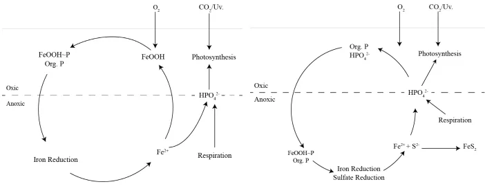
sulfate reduction can result in the decoupling of iron from the phosphorus cycle shown in Figure

2-7. This can enhance the trophic status, as the phosphorus is used in primary productivity and

algal growth, leading to eutrophication (Hupfer, 2008).

(36)

[image:36.842.93.795.68.344.2]

Figure 2-7: Iron, Phosphorus and Sulfur cycles (modified from Hupfer (2008)).

The coupling of the iron and phosphorus cycles related to the sediment-water interface and the change in redox potential with depth (Figure 2-7). In the right hand component of Figure 2-7, the decoupling of the iron and phosphorus cycles due to sulfate reduction, a result of elevated sulfate concentrations. Sulfide produced from sulfate reduction results in the sequestration of iron in the sediments and the flux of iron is minimised. The result is the release of phosphorus to the overlying water column. The liberation of phosphorus into the overlying water column may enhance the trophic status of the wetland, possibly resulting in eutrophication.

(37)

2.4.4. Nitrogen Cycling

Coupled with phosphorus, nitrogen is another important nutrient in biogeochemical cycling. The

cycling of nitrogen is considerably more complex than the cycling of other elements due to

nitrogen being a major constituent of the atmosphere, with 78% composed of N2, as well as being

an essential component of living tissue in both animals and plants. The nitrogen cycle is shown

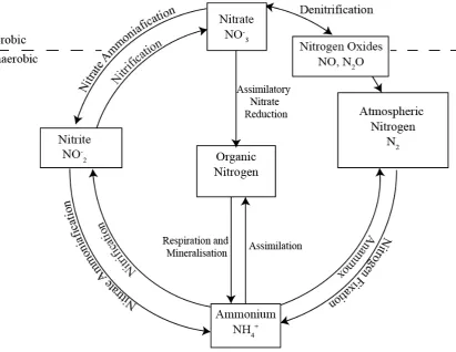
[image:37.595.115.527.203.521.2]

diagrammatically in Figure 2-8.

Figure 2-8: Nitrogen Cycle

The nitrogen cycle involves assimilatory and dissimilatory incorporation of nitrogen into organic carbon. Nitrogen can be transformed by bacteria and plants into ammonia, nitrate, nitrite, nitrogen gas, and nitric and nitrous oxides Modified from Reddy and DeLaune (2008) .

Elemental nitrogen (N2) is very unreactive due to the strong triple bond in the molecule, as noted

previously. Despite the unreactive nature of molecular nitrogen, there are some bacteria

(Azotobacter, Rhizobium and Clostridium spp.) and certain cyanobacteria that are able to fix

nitrogen and assimilate it as organic nitrogen shown in Equation 2.33 (Reddy and DeLaune, 2008;

Stumm and Morgan, 1996):