Depth-Map-Assisted Texture and Depth Map Super-Resolution

(1)

Depth-Map-Assisted Texture and Depth Map

Super-Resolution

Thesis submitted in accordance with the requirements of the University of Liverpool for the degree of Doctor in Philosophy

by

Zhi Jin

Department of Electrical Engineering and Electronics

School of Electrical Engineering and Electronics and Computer Science University of Liverpool

Supervisor team: Prof. Tammam Tillo (Xi’an Jiaotong-Liverpool University) Dr. Waleed Al-Nuaimy (University of Liverpool)

(2)

Abstract

With the development of video technology, high definition video and 3D video

applica-tions are becoming increasingly accessible to customers. The interactive and vivid 3D

video experience of realistic scenes relies greatly on the amount and quality of the

tex-ture and depth map data. However, due to the limitations of video capturing hardware

and transmission bandwidth, transmitted video has to be compressed which degrades,

in general, the received video quality. This means that it is hard to meet the users’

re-quirements of high definition and visual experience; it also limits development of future

applications. Therefore, image/video super-resolution techniques have been proposed

to address this issue.

Image super-resolution aims to reconstruct a high resolution image from single or

multiple low resolution images captured of the same scene under different conditions.

Based on the image type that needs to be super-resolved, image super-resolution

in-cludes texture and depth image super-resolutions. If classified based on the

implemen-tation methods, there are three main categories: interpolation-based,

reconstruction-based and learning-reconstruction-based super-resolution algorithms. This thesis focuses on

exploit-ing depth data in interpolation-based super-resolution algorithms for texture video and

depth maps. Two novel texture and one depth super-resolution algorithms are proposed

as the main contributions of this thesis.

The first texture super-resolution algorithm is carried out in the Mixed Resolution

(MR) multiview video system where at least one of the views is captured at Low

Reso-lution (LR), while the others are captured at Full ResoReso-lution (FR). In order to reduce

visual uncomfortableness and adapt MR video format for free-viewpoint television, the

low resolution views are super-resolved to the target full resolution by the proposed

virtual view assisted super resolution algorithm. The inter-view similarity is used to

determine whether to fill the missing pixels in the super-resolved frame by virtual view

(3)

tex-ture characteristics of the neighbors of each missing pixel. Thus, the proposed method

can recover the details in regions with edges while maintaining good quality at smooth

areas by properly exploiting the high quality virtual view pixels and the directional

correlation of pixels. The second texture super-resolution algorithm is based on the

Multiview Video plus Depth (MVD) system, which consists of textures and the

as-sociated per-pixel depth data. In order to further reduce the transmitted data and

the quality degradation of received video, a systematical framework to downsample

the original MVD data and later on to super-resolved the LR views is proposed. At

the encoder side, the rows of the two adjacent views are downsampled following an

interlacing and complementary fashion, whereas, at the decoder side, the discarded

pixels are recovered by fusing the virtual view pixels with the directional interpolated

pixels from the complementary downsampled views. Consequently, with the assistance

of virtual views, the proposed approach can effectively achieve these two goals. From

previous two works, we can observe that depth data has big potential to be used in 3D

video enhancement. However, due to the low spatial resolution of Time-of-Flight (ToF)

depth camera generated depth images, their applications have been limited. Hence, in

the last contribution of this thesis, a planar-surface-based depth map super-resolution

approach is presented, which interpolates depth images by exploiting the equation of

each detected planar surface. Both quantitative and qualitative experimental results

demonstrate the effectiveness and robustness of the proposed approach over benchmark

(4)

List of Tables

3.1 The PSNR differences (dB) between the FR and LR views using H.264

for: (a) Bookarrival; (b) Doorflower; (c) Laptop; (d) Champagne with

QP = 22, 27, 32, 37, 42, 47 . . . 45

3.2 The parameters and characteristics for each used sequence . . . 53

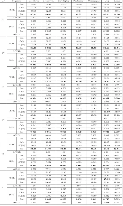
3.3 The Luminance PSNR (dB) and SSIM results of proposed method in

comparison with other methods and corresponding gains of the proposed

method over Lanczos method . . . 55

3.4 PSNR (dB) and SSIM of SR results obtained by the proposed method

and reference method in[1] . . . 57

3.5 The Luminance PSNR gain (dB) and SSIM gain for each stage of the

proposed approach;“zfvf” and “zfve” stand for zero-filled view filling

stage and the enhancement stage, respectively . . . 58

3.6 The Luminance PSNR (dB) and SSIM values and gains over the

bench-mark method for multiview video . . . 60

4.1 The parameters and characteristics of each used sequence . . . 73

4.2 The values ofηh,ηv,η45,η135and ηudfor each sequence and for different

QPs . . . 79

4.3 The upsampling performance on PSNR (dB) and SSIM comparison by

discarding even rows directly downsampling . . . 81

4.4 The PSNR (dB) comparison between: derivingη values for each frame,

using theη values of first frame and user definedη values for the whole

sequence . . . 83

5.1 The measured angle of each tooth in the 3D saw-tooth structure by the

proposed approach with and without the post-processing (PP) stages;

(8)

5.2 The ROC of the proposed algorithm with and without the post-processing

(PP) stages for some planar surfaces of a 3D saw-tooth structure; “TP”,

“TN”, “FN”, and “FP” stand for True Positive, True Negative, False

(9)

List of Figures

1.1 The image acquisition process. . . 2

2.1 The working principle of digital camera [2]. . . 9

2.2 Testing image Lenna (a) and RGB values on the two highlighted parts.

(b) the RGB values on white square region; (c) the RGB values on black

square region. . . 10

2.3 The Bayer color filter mosaic. (a) The Bayer arrangement of color filters

on the pixel array of an image sensor; (b) cross-section of sensor. . . 11

2.4 Low resolution images acquisition [3]. . . 11

2.5 Working principle of stereo matching method. . . 14

2.6 (a) ToF laser range finder scanner; (b) NextEngine 3D Scanner

(trian-gulation 3D laser scanners). . . 15

2.7 ToF detection system. . . 16

2.8 Received sinusoidally modulated input signal, sampled with 2 sampling

points per modulation period T. . . 17

2.9 Classification of SR problems and approaches. . . 19

2.10 Block diagram of the SR observation model. . . 20

2.11 Using nearest neighbor to interpolate a checkerboard image. (a) the

original LR image with size 2×2, (b) the interpolated HR image with

size 176×144. . . 22

2.12 Comparison between common used interpolation methods. (a) the

orig-inal LR image with size 53×49, the interpolated results of HR image

with size 176×144 by using (b) nearest neighbor, (c) bilinear and (d)

bicubic. In order to have a clear view of the original LR image, it has

been shown in the same size as the other three images. . . 22

(10)

2.14 The working principle of bicubic interpolation. . . 24

2.15 The interpolation results of (a) bicubic method (b) [4], (c) [5] and (d)

[6] interpolate the 128×128 lena to 256×256. . . 26

2.16 Training process. . . 28

2.17 First row: an input patch; middle row: similar low-resolution patches;

bottom rows: paired high-resolution patches. For many of these

simi-lar low-resolution patches, the high-resolution patches are different from

each other [7]. . . 29

2.18 SR approach for multiview images. A super-resolved image ˆVnis created

from its low-resolution version,V_nD, a neighboring HR view, Vk, and the

depth information for each of these views,Dn andDk [8]. . . 31

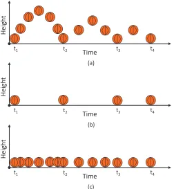
2.19 Temporal aliasing. (a) Trajectory of a ball over time. (b) Trajectory

sampled over time by a low frame rate camera. Perceived trajectory

is along a straight line. (c) Illustration that even with ideal temporal

interpolation of (b) the true motion trajectory cannot be recovered. . . . 33

2.20 (a) framework consists of a 3D-ToF camera, SR4000 and a RGB camera

(b) Microsoft developed depth camera, Kinect. . . 35

3.1 The framework of the proposed super-resolution method. . . 40

3.2 A pictorial representation of the similarity check process and the

gener-ation of FR frame. . . 42

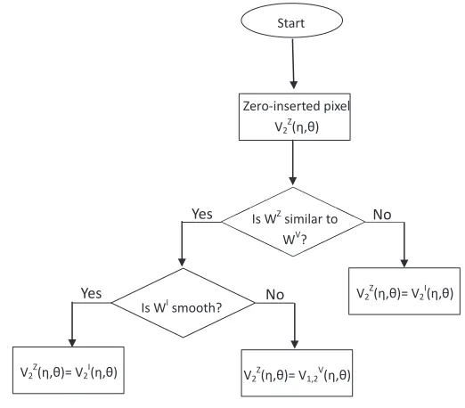
3.3 Flowchart of the Zero-filled View Filling stage. . . 44

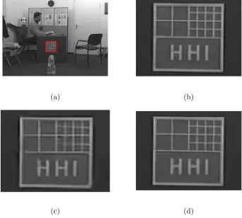
3.4 Comparison of the effect of luminance compensation on the first frame

of “Pantomime” and “Bookarrival” sequences. The two images on the

left show the artifacts in the super-resolved frames without luminance

compensation and the two images on the right show the visual effects of

same frame but after luminance compensation (better perception could

be achieved by viewing the images at their full resolutions, which are

620×775 for (a) and (b); 620×884 for (c) and (d)). . . 45

3.5 The comparison of exhaustive and successive approaches for thresholds

(11)

3.6 PSNR and SSIM comparisons of different approaches for the evaluation

ofαandβ; (a) and (b) are results of “Doorflower”; (c) and (d) are results

of “Pantomime”. . . 52

3.7 The proposed algorithm for multiview multi-resolution system. . . 52

3.8 (a) the reference FR frame; (b) cropped portion of the FR frame; the

results at QP=32 for: (c) benchmark interpolation method; (d) proposed

method; full resolution of the cropped portion is 620×884. . . 56

3.9 The PSNR value for each 8×8 block evaluated on the luminance

compo-nent of the first frame of “Doorflower” (shown in Fig.3.8 (a)) at QP=22.

(a) benchmark interpolation method; proposed method: (b) after

simi-larity check, (c) after smoothness check, and (d) after enhancement stage. 57

4.1 The proposed interlacing-and-complementary-row-downsampling process

for a stereo video. . . 64

4.2 (a), (b) and (c) show the front, side, and top view of the stereoscopic

orthographic projection of uneven bars structure viewed by two cameras

in a parallel configuration setting, as shown in (d). . . 65

4.3 (a) the left side and right side of each frame shown the captured scene

by the corresponding cameras, respectively; (b) the output of the

ver-tical downsampling approach (i.e., column-wise downsampling); (c) the

output of the interlacing and complementary row-wise downsampling. . . 66

4.4 The top view of the prospective projection of a scene using a pinhole

camera model for the column-wise downsampling approach. . . 66

4.5 The proposed discarded pixels recovery process. . . 68

4.6 The overlapping window centered at the discarded pixelp5. The

domi-nant pattern direction will be categorized into five groups. In this figure

only the remarkably dominant patterns are shown which are horizontal,

45○ diagonal, vertical and 135○ diagonal directions. . . 70 4.7 The process of data fusion by directional weighting coefficients and

cor-responding directional binary masks . . . 73

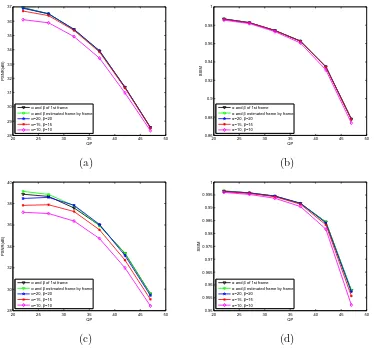
4.8 The rate-distortion curves for the testing sequences (a) Doorflower; (b)

(12)

4.9 The rate-distortion curves for the testing sequences (a) Doorflower; (b)

Laptop, for the proposed approach and [9]. . . 76

4.10 Comparison between proposed DDFU method and benchmark method.

(a)-(c) are the results of Original, Benchmark and DDFU on

zoomed-in part of the sequence Doorflower; (d)-(f) are the results of Origzoomed-inal,

Benchmark and DDFU on zoomed-in part of the sequence Undo-Dancer. 77

4.11 (a) original texture; the pattern direction estimation results on: (b)

original uncompressed texture; (c) compressed texture with QP=34; (d)

compressed texture with QP=40; the color: dark red, red, orange, yellow

and white represent vertical, 135○ diagonal, horizontal, 45○diagonal and undefined direction pixels, respectively. (For clearness, the directional

estimation results on the discarded pixels are scaled up to the same size

as the original texture; their real height is shown on the y axis of each

figure). . . 78

4.12 (a) and (b) panes show the four coefficients for the sequence

“Doorflow-ers” and “Dog”, respectively. The top Left and Right figures of each

pane are: the weighting coefficients of Left and Right view, respectively,

when QP=28; The bottom Left and Right figures of each pane are: the

weighting coefficients of Left and Right view, respectively, when QP=46. 82

5.1 The framework of the proposed depth map based planar surface detection

method. . . 90

5.2 An example of the growing process of a planar surface;Dis depth map,

S_ij is the current surface andN_ij is current neighboring pixels. . . 92 5.3 Two typical cases of overgrowing surfaces: (a) lateral-OGS; (b)

axial-OGS; the lateral points and medial points of the OGS are shown in

green and red, respectively. . . 93

5.4 (a) and (b) are the examples of daily life scenes with OGS problem; red

(13)

5.5 (a) shows two intersecting surfaces ¯Si and ¯Su; (b) the overgrowing

sur-faceSi splitting ¯Su into two surfaces; the scanning element is shown in

violet; (c) the detected shared surface (So) is shown in green; (d) the

outcome of relocating the shared surface when processingSi and Su; (e)

the outcome of relocating the shared surface when processingSi andSk;

(f) the outcome of fragmented element relocation and finalizing surfaceSi. 95

5.6 The flowchart of the proposed OGS algorithm. . . 98

5.7 The framework of the proposed depth map super-resolution method. . . . 100

5.8 The capturing texture and depth camera platform: (a) front view; (b)

side view . . . 103

5.9 Detection comparison of the proposed DPSD method and benchmark

method for several scenes. Each of the four panes is as follows: Top Left:

the original texture of the scene. Top Right: the corresponding depth

map. Bottom Left: detection results of benchmark method. Bottom

Right: detection results of proposed method. . . 105

5.10 The outcome of the proposed approach: (a) without any of the two

post-processing stages; (b) with only the OGS post-post-processing stage; (c) with

the two post-processing stages. . . 106

5.11 The results of each tested scene are shown in one pane; the columns

from left to right in each pane show the results for 3×3, 4×4, and 5×5

seed patch; the upper and lower row of each pane show the output of the

proposed approach with and without post-processing stages, respectively. 107

5.12 (a) The 3D saw-tooth structure, each “tooth” has different height; (b)

the profile of the saw-tooth structure with the angle of each tooth is

shown on its top. . . 108

5.13 The detected planner surfaces by the proposed algorithm: (a) with the

post-processing stages; (b) without the post-processing stages. The

ac-tual intersection lines between each two surfaces are shown as dashed

lines. . . 108

5.14 The row-by-row MSE for the up-sampled saw-tooth image with respect

(14)

5.15 Image (a) shows the original LR 176×144 depth image; the output of the

surface categorization is shown in (b), where horizontal hatch pattern

shows planar surfaces; the edges and the isolated non-filled pixels are

shown in (c). . . 111

5.16 The super-resolved image using: (a) proposed approach; (b) traditional

interpolation approach; The delimitated area by a red box in (a) and (b)

(15)

List of Abbreviations

CCD Charge Coupled Device

CFA Color Filter Array

CG Computer Graphic

CMOS Complementary Metal Oxide Semiconductor

CS Compressive Sensing

DDFU Directional Data Fusion Upsampling

DIBR Depth Image-Based Rendering

FN False Negative

FP False Positive

FR Full Resolution

FRUC Frame Rate Up-conversion

F-SFM Factorization Structure From Motion

FTV Free-viewpoint Television

GOP Group of Pictures

HDTV High Definition TV

HR High Resolution

(16)

IBP Iterative Back Projection

JBU Joint Bilateral Upsampling

LCC Local Coordinate Coding

LLE Locally Linear Embedding

LMMSE Linear Minimum Mean Squares-error Estimation

LR Low Resolution

LSI Linear Space Invariant

LSV Linear Space Variant

MAD Mean Absolute Deviation

MAP Maximum A Posteriori

MDL Minimum Description Length

ML Maximum Likelihood

MR Mixed Resolution

MRF Markov Random Field

MSE Mean Square Error

MSFE Mean Square Fitting Error

MVD Multiview Video plus Depth

(17)

PAR Piecewise Autoregressive

PCA Principal Components Analysis

POCS Projection Onto Convex Sets

PSD Planar Surface Detection

PSF Point Spread Function

PSNR Peak Signal to Noise Ratio

QP Quantization Parameters

RANSAC RANdom SAmples Consensus

REoD Relative Error of Depth

RGB Red Green Blue

SFM Structure From Motion

SR Super-Resolution

S-SFM Sequential Structure From Motion

SSIM Structural Similarity

SSSIM Structural Self-Similarity

SVD Singular Value Decomposition

SVR Support Vector Regression

ToF Time-of-Flight

TN True Negative

(18)

Write your injuries in dust, your benefits in marble.

Benjamin Franklin, Statesman

Acknowledgement

The past four years of my Ph.D. research was an unforgettable and valuable experience

which was full of happiness, laughter, anticipation, satisfaction, and also sadness,

anx-iety, disappointment, frustration. It consisted of many hardworking days and nights,

and tears of success and failure. For sure, all of these would not happen without the

help of numerous people, all of who I would like to remember with appreciation during

my whole life.

First and most importantly I would like to express my heartfelt gratitude to my

Ph.D. supervisor, Professor Tammam Tillo for his unwavering and helpful supports

not only of my research but also my life, for his kindness, encouragement, spontaneous

guidance, patience, comfort, understanding, tolerance, foresight from the first day I

became his student, six years ago and then through every stage in this long journey.

He spent many hours editing and improving the readability and presentation of my

thesis as well as my academic papers. He tried his best to provide me with both

economic and academic support to attend international conferences. To express all

of my gratitude to him, I need many pages. In short, because of him, such kind of

supervisor, I feel I am a lucky Ph.D. student. Besides my primary supervisor, I would

like to thank my co-supervisor Dr. Waleed Al-Nuaimy, in University of Liverpool, UK.

My sincere thanks also go to Dr. Jimin Xiao, the senior Ph.D, now lecturer in our

group, who not only discussed research with me, but also helped me modify my papers

and this thesis; Professor Byeungwoo Jeon, in Sungkyunkwan University, Korea and

Professor Eckehard Steinbach, in Technical University of Munich, Germany, for

giv-ing me chances studygiv-ing in their research groups and learngiv-ing from other outstandgiv-ing

Ph.D. students; Professor Yao Zhao, who supports me as the leader of our solid research

partners in Beijing Jiaotong University including Yao Chao; Professor Mark Leach, in

our department who helped me modify this thesis during his Christmas holiday and

(19)

in the Multimedia Technology lab and Department of Electrical and Electronics

En-gineering, especially Fei Cheng who provides lots of hardware supports. I thank all

of my teachers, students, friends, relatives and all others who helped and inspired me

directly or indirectly, and all who have wished me well in my study, research and other

purposes. Special thanks to my teacher V.K. Liau who taught me how to become a

valuable and useful person in the world and the truth of our life.

My eternal gratitude goes to my parents for their unconditional love, and who have

always tried to make my life comfortable, always wish me for success and happiness

from the moment I came to the world. They suffer from their missing in order to give

me the freedom to explore the lovely world. They work hard in order to make me never

worry about money. They try their best to live happily and healthily in order to make

me do not worry about them. All of these are the light and power for me to walk

further in my life.

Last but not least, I would like to thank Xing Luo. Without him, I could finish this

(20)

Chapter 1

Introduction

1.1 Motivation

The development of video technologies make high definition video and 3D video

appli-cations increasingly accessible to consumers through products, such as, High-Definition

(HD) TVs, computer monitors, HD cameras, smart phones, and many other handheld

devices. However, the demands for High Resolution(HR) and 3D video put pressure on

the acquisition, storage and transmission processes, especially for bandwidth limited

applications [10]. Hence, the popularity of HR or 3D video in the multimedia market

still faces many challenges.

Perceived image quality relies greatly on the capture and delivery process. For

im-age quality assessment, one essential factor is spatial resolution (or pixel density) in

one image, which is affected by the camera sensor (e.g., Couple Charge Device (CCD))

[2] [3]. High resolution images can be obtained by increasing the total number of pixels

on a CCD chip either via reducing pixel size or increasing chip size. Whereas, the

effectiveness of the first approach is limited by shot noise which severely degrades the

image quality. The second approach increases chip size, on one hand, it will lead to

an increase in capacitance which will decrease the charge transfer rate. On the other

hand, it will cause an additional increase in cost due to the high precision optics and

image sensors required [3]. In spite of the limitations of the camera sensor, in reality,

due to the capture conditions and digital camera techniques, the captured images

usu-ally cannot reflect all of the information in a scene. The image acquisition process is

shown in Fig.1.1, where the atmosphere turbulence, the motion transformation caused

distortion, the downsampling introduced distortion and the hardware caused additive

(21)

especially HR images, requires much higher bitrate than text, before transmitting,

high compression rates are required, resulting in annoying compression artifacts, such

as, block artifacts, blurred details and ringing artifacts around edges [12]. Therefore,

a new approach toward increasing spatial resolution, so as to increase the quality, is

needed. One effective solution to solve these kinds of problem is the super-resolution

technique, which could provide a cost-effective solution to increase image resolution.

Original

scene Transformation

Blur

effect Downsampling

Actual captured image Noise

Figure 1.1: The image acquisition process.

Since Super-Resolution(SR) techniques are targeted at increasing the spatial

reso-lution of low-cost hardware obtained LR images and limited bandwidth obtained LR

images by using software, they have played an important role in many applications. For

example, in surveillance video applications, SR can be used to obtain higher quality

video sequences from several low resolution cameras [13] and to recognize car license

plates and faces robustly and efficiently even under bad capture conditions [14] [15].

In the remote sensing and astronomy fields, due to the size and weight limitation of

satellite cameras, power supply and transmission bandwidth, the obtained images are

usually in low resolution. Therefore, SR techniques become essential for earth

en-vironment observation [16]. Medical imaging has become an important aid tool for

medical diagnosis. Using SR to enhance the quality of medical images, the condition

and position of a lesion can be well determined, so that the accuracy of diagnoses can

be improved [17]. In consumer electronics, entertainment and digital communication

applications, multimedia content occupies a dominant share. SR techniques can offer

an improved viewing experience for customers by enlarging the resolution of perceived

images/video and removing the visual artifacts caused by video compression [18].

More than 30 years ago, researchers began to work on extracting information from

multiple digital images to enhance the spatial resolution of LR images [19]. In general,

the SR algorithms for images can be mainly classified into 3 categories:

reconstruction-based algorithms [20], learning-reconstruction-based algorithms [7][21] and interpolation-reconstruction-based

algo-rithms [22][23]. Techniques in the first category are based on the assumption that

(22)

ap-proaches can be realized in both the frequency and spatial domains [24] [25]. However,

this kind of method highly relies on the choice of the regularization parameters and the

number of LR images, which are not easy to obtain in reality [26]. In contrast,

learning-based SR approaches assume that it is possible to predict the missing high frequency

details in a single LR image by a group of LR and FR image pairs [27]. Since image

information hides underlying models, it can be modeled as a mathematical function.

Unfortunately, their performance largely depends on the choice of training samples,

so unsuitable training samples can produce artifacts in the recovered High Resolution

(HR) image [26]. Free from the suffering from the dependency problem on training

data and having well time performance, especially for real time systems,

interpolation-based SR algorithms are widely adopted. The interpolation-interpolation-based SR algorithms are

implemented based on the fact that the missing HR pixels can be estimated by using

the information from neighboring LR pixels. However, the main drawback of these

methods is their inability to fully exploit the scene content during the interpolation

process, and consequently they are prone to blur high frequency details (edges).

1.2 Objectives

The main goal of the thesis is to propose specific and sophisticated interpolation-based

3D SR solutions for different purposes, so that to fill the gaps with respect to current

2D SR algorithms. With one more cue in depth, the SR methods designed for 3D video

can achieve better results than directly applying 2D SR algorithms on 3D video. To

fulfil this objective, the research work was carried out by introducing depth information

into the SR process. However, the depth camera generated depth images have lower

resolution than the corresponding textures which makes them cannot be used directly.

Hence, the depth camera generated depth images need to be super-resolved to the same

resolution as the textures. To achieve the final goal, this thesis addresses the following

objectives:

• Providing a review of classic and the state-of-the-art 2D SR methods as the

general background.

• Developing a 3D SR algorithm for 3D-MR video.

(23)

• Developing a robust and accurate planar surface detection algorithm on the depth

camera generated depth images.

• Developing an efficient depth image SR algorithm based on the planar surface

(24)

1.3 Overview of this thesis

1.3.1 Contribution of This Thesis

This thesis provides an investigation of efficient texture and depth image SR algorithms

for different applications by using depth information. The main contributions of the

thesis are:

• Depth-map-assisted texture super-resolution for multiview mixed-resolution

video system

A new virtual-view-assisted SR and enhancement algorithm is proposed, where

the exploitation of the virtual view information and the interpolated frames

of-fers two benefits. Firstly, the high frequency information contained in the FR

views can be properly utilized to super-resolve LR views; secondly, the inter-view

redundancy is used to enhance the original LR pixels in the super-resolved views

and to compensate for the luminance difference between views. The

experimen-tal results show that the proposed algorithm achieves superior performance with

respect to interpolation-based algorithms. This work was published in [28], and

is presented in Chapter 3.

• Depth-map-assisted texture super-resolution for multiview video plus

depth system

In Chapter 3, the FR views generated virtual views and traditional interpolated

views are used in conjunction to super-resolve the LR view in a multiview

mixed-resolution video system. While, in this framework, in addition to super-resolving

one LR view, the two FR views are downsampled before encoding and

super-resolved after decoding by exploiting inter-view redundancy via virtual views.

In the proposed downsampling approach, the rows of two adjacent texture views

are discarded following an interlacing and complementary pattern, before

com-pression. The aim of this downsampling approach is to systematically facilitate

the resolution task at the decoder end, where the LR views will be

super-resolved by fusing the virtual view pixels with directional interpolated pixels with

the aid of pattern direction of the discarded pixels. This approach has two

bene-fits. Firstly, the high frequency information contained in the counterpart LR view

(25)

virtual views. Secondly, since the virtual view quality depends on many factors,

including the DIBR technique and depth map quality, it generally has low quality

in areas where the corresponding depth data suffers from discontinuities. On the

other hand, directional interpolation approaches can work well. Hence, by taking

advantage of these two kinds of strategy, the discarded pixels can be recovered

efficiently. The experimental results have shown that the proposed algorithm

achieves superior performance with respect to the filter-based interpolation

al-gorithms and state-of-the-art alal-gorithms. This work could be regarded as an

extension of the work presented in Chapter 3.

• Super-resolution of depth map by exploiting planar surfaces

In the previous chapters, depth data has shown the big potential to be used to

super-resolve LR views and the techniques of generating depth map become more

mature and accurate. However, the ToF depth camera generated depth maps

still suffer from low resolution. Therefore, in Chapter 5, this thesis focuses on

depth map SR by exploiting planar surfaces on a single depth map. In this way,

the super-resolved depth maps can expand the application domains of texture SR

algorithm.

Depth maps, different from common texture images due to their large

homoge-neous areas, are delimitated by sharp edges at the discontinuities between objects.

After projecting 3D objects, they can be represented by several planar surfaces

with different shapes in a 2D image, each surface will have linearly changing depth

values in the corresponding depth map and the boundaries of surfaces represent

the discontinuities of the depth values. If the equation of each surface can be

obtained, the SR of the LR depth map can be obtained by inserting pixels based

on this equation. Therefore, the whole depth map can be classified into three

categories: planar surfaces, non-planar surfaces, and edges. In [29], the SR of

depth map relied on the local planar hypothesis and the candidates for potential

HR depth values were obtained by either linear interpolation along horizontal

and vertical directions or the estimated local planar surface equations. However,

since the surface equation was evaluated locally, it may be biased by noise

affect-ing local pixels which later on will magnify the estimated error of the generated

(26)

of global analytical equations of the detected surfaces in the scene. For each of

these three categories a proper up-sampling approach is proposed to exploit its

intrinsic properties. The related work was published in [30] [31], and is presented

in Chapter 5.

1.3.2 Organization of This Thesis

This thesis is organized as follows: Chapter 2 provides general background on image

acquisition and assessment. The advantages and challenges of current SR algorithms are

reviewed and discussed. Then, the related concepts and techniques are also introduced.

Chapters 3 and 4 give the details of the two proposed texture SR algorithms,

re-spectively, while Chapter 5 changes the focus to the depth map SR algorithm. Chapter

6 summarizes the whole thesis and discusses possible future research directions in the

(27)

Chapter 2

Background

2.1 Introduction of Texture Image

2.1.1 Texture Image Acquisition

The history of the first generation of the photographic camera dates back to the fifth

century B.C. Its working principle, camera obscura, was discovered by the Chinese

philosopher Mo Di [32]. However, it was not until 1826 when the first permanent

photographic image from a camera obscura was captured by Joseph Nicphore Nipce

on a bitumen-coated metal plate. From that time the floodgates of using photographs

to record human actions were opened. Subsequently many recording techniques have

been developed, themselves diverse in nature and in many cases easier to use than

before. In 1888, Kodak invented a new photographic material, photographic film,

and produced the first photographic film camera. The invention of photographic film

greatly improved the usage of the camera. In 1975, the first digital camera was invented;

formally heralding the human progression into the digital imaging era.

The working principle of the digital camera is completely different from that of

the conventional camera. A conventional film camera captures the image based on

chemical reactions that take place in an emulsion covering the surface of the film when

it is exposed to light. The emulsion is commonly composed of silver salt, whose particles

are sensitive to the quantum effect of light. The spatial variations of light intensity are

captured in the salt and appear after developing the film. Instead of using a chemical

approach, the digital camera relies on a physical approach, using electronic sensors to

perceive spatial variations in light intensity. With the aid of some image processing

algorithms, the sensor data is converted into color images and stored in a visible digital

(28)

image sensor

recovery engine

illumination

lens

scene

color engine input

processor

anti-vignette,

spatial -distortion

encoding

imaging

[image:28.595.159.437.74.286.2]

array color filterarray

Figure 2.1: The working principle of digital camera [2].

Currently, there are two major types of imaging sensor, namely CCD (Charge

Cou-pled Device) and CMOS (Complementary Metal Oxide Semiconductor). The CCD

consists of tiny light-sensitive diodes, called photosites, which can convert photons into

electrons [33]. In this way, light can be represented by electrical charge. The brighter

the light on a single photosite, the greater the electrical charge that will accumulate

at that photosite. The CMOS imaging chip, as a kind of active pixel sensor, is made

by semiconductors. Both types of image sensor can convert light into electrons at the

photosites and then an analog-to-digital converter will turn each pixel’s value into a

digital value. CCD sensors have the ability to accumulate the charges and extract

them from the chip without distortion, therefore, CCD sensors have high fidelity and

light sensitivity and also have been widely used in professional, medical, and scientific

applications where high-quality image data is required. On the other hand, CMOS

sensors with a more consolidated manufacturing process have a lower price and quality

than that of CCD sensors. Hence, for applications with less demand on quality, such

as consumer digital cameras, the CMOS sensor is popular [34].

On these sensors, each sensitive element can be called a “pixel” and the pixel is the

basic unit in a digital image. In general, the number of pixels in each dimension of a

rectangular image represents the spatial size of an image in that dimension (known as

resolution) and the per-unit quality of captured images is determined by the number

(29)

be recorded in the captured image. For example, nowadays the popular HDTV (High

Definition TV) which has a resolution of 1920×1080 means that each frame has 1920

and 1080 pixels along the horizontal and vertical directions, respectively. In texture

images, each pixel consists of three color components, Red, Green, and Blue (RGB).

The perceived color differences are caused by mixing these three components with

various intensities. An example is shown in Fig.2.2, two crops from the color image

Lenna have different values of the RGB components.

(a) (b) (c)

Figure 2.2: Testing image Lenna (a) and RGB values on the two highlighted parts. (b) the RGB values on white square region; (c) the RGB values on black square region.

In the common configuration each sensor element responds to one colour component

only, hence there is a Color Filter Array (CFA) in the digital camera, located on the

top of the sensor array, to decompose incoming light into the three primary colors.

One common CFA arrangement pattern is called the Bayer pattern [35]. As shown in

Fig.2.3, the number of green mosaics is twice the number of the red and blue mosaics.

This is due to the fact that the Human Vision System (HVS) is more sensitive to the

color green than the other two. At each pixel position, there is only one color intensity,

hence, the values for the other two missing colors are interpolated from the adjacent

corresponding colors. This process is known as “demosaicing”. Each pixel is to be an

RGB triplet. After some post-processing procedures, the captured images are stored

in a digital storage device.

In the process of capturing a digital image, there are some factors that affect the

quality of the obtained images. For example, optical distortions affect spatial resolution,

limited shutter speed causes the motion blur effects and the camera sensors result in

(30)

/ / g

(a)

Incoming light

Filter layer

Sensor array

Resulting pattern

_ _

(b)

Figure 2.3: The Bayer color filter mosaic. (a) The Bayer arrangement of color filters on the pixel array of an image sensor; (b) cross-section of sensor.

aliasing effects (Fig.2.4).

Common Imaging System

Original Scene Blurred, Noisy,

Aliased LR Image Environment

OTA

CCD Sensor Preprocessor

Optical Distortion

Aliasing Motion Blur Noise

Figure 2.4: Low resolution images acquisition [3].

2.1.2 Texture Quality Assessment

In image transmission systems, between being captured and being received, the image

passes through many steps and the techniques adopted in these steps may result in an

aggregate degradation of the visual quality of the final received image. The SR approach

is one of the image post-processing techniques, aimed at improving image quality. In

order to quantify the received image quality and the efficiency of SR approaches, some

quality assessment methods are required.

Assessment of the quality of an image can be carried out objectively or

subjec-tively, each of which has its own strengths and associated applications. The objective

image quality assessment is usually focused on two aspects: fidelity and intelligibility

(31)

origi-nal image”. It mainly focuses on the detailed differences in the two images and the

higher the fidelity is, the better the image quality is. While, intelligibility is used to

indicate “how well the image can deliver the original information to its viewers in spite

of the distortion affecting the image”. It focuses on the global quality of the received

images. Many researchers have worked on these two factors and tried to develop

quan-titative measures that can accurately describe the perceived image quality. To date, the

objective quality assessment approaches can be classified into: ground truth approach

which uses the available original image, and those are called the full-reference approach;

the no-reference approach which uses no original image, and the reduced-reference

ap-proach which uses only part of the original image (e.g. the region of interest). For

the full-reference approach, since the original image is known, it is more

straightfor-ward to measure the quality. The most widely used full-reference quality assessment

metrics are the Mean Squared Error (MSE), Peak Signal-to-Noise Ratio (PSNR) and

Structural Similarity (SSIM). These assessment metrics are popularly used in many

applications mainly due to their computational simplicity, clear physical meanings and

the mathematical convenience in the context of optimization. However, in many

prac-tical applications, the reference image is not available, and the no-reference or blind

quality assessment approach is desirable.

For an original image, IGT with size W ×H, the quality of a received image I

measured by MSE is:

M SE=

W

∑

i=1

H

∑

j=1(

IGT(i, j) −I(i, j))2

W ×H (2.1)

The quality of a received image I measured by PSNR can be calculated through

MSE:

P SN R=10 lg( B

2

M SE) (2.2)

where B represents the quantization level. In general, 8-bit images have pixel values

within the range [0,255], B = 255. Since either MSE or PSNR globally measures

an image similarity to the original one by averaging the intensity differences between

pixels, they do not provide assessment results consistent with the perceived visual

quality. Thus, Wang et al. [37] proposed the SSIM matrix to assess image quality based on the image structure information at the pixel level. The quality of received

(32)

SSIM(x, y)= (2µxµy+c1)(2σxy+c2) (µ2

x+µ2y+c1)(σx2+σ2y+c2)

(2.3)

For each pixel (x, y) within the N ×N windows Wx and Wy, its mean value and

variance for window Wx are µx and σx2, respectively and for window Wy, are µy and

σ_y2, respectively. σxy is the covariance of pixels within Wx and Wy and c1 and c2 are

two constant values. The final SSIM result is obtained by averaging all values.

Since the received image/video is finally viewed by a human, then subjective

eval-uation is more “proper” to quantify visual image quality than objective evaleval-uation. In

practice, however, subjective assessment requires a human participant which makes it

inconvenient, time-consuming and expensive. Hence, some advanced objective

assess-ment approaches are needed.

2.2 Introduction of Depth Map

Depth map is a grey image with each pixel value between 0 and 255. Larger the pixel

value is, closer this point to the depth camera. Hence, depth map can represent the

relative distance between objects in a scene and the capturing depth camera. Due to

this feature, it has been widely utilized in 3D applications to provide an immersive 3D

and free-viewpoint experience for the viewer.

In this section, firstly, various depth map acquisition methods will be described,

highlighting their corresponding weaknesses. The quality assessment methods and some

useful depth map applications will also be introduced.

2.2.1 Depth Map Acquisition

Depth maps can be generated using software or hardware driven techniques, such as

stereo or multiview matching-based methods, Structure-from-Motion (SfM), 3D laser

scanner and depth-camera-based methods [38].

Since depth maps have many applications in computer vision and visual perception

field, various software-based algorithms which compute correspondences from stereo

or multiple views, have been proposed for the acquisition of depth map [39]. Stereo

matching and SfM are two common depth map estimation methods in the computer

vision field and since they do not rely on active illumination, they are regarded as

(33)

x r x l Z X b f

X+b

2 X b 2 x f X b Z l ₌ + 2 x f X b Z

r ₌ 2

x x b

Z

2 b

]

Figure 2.5: Working principle of stereo matching method.

Matching-based methods require at least two color images of the same scene

cap-tured from slightly different viewpoints. The common features and areas in these two

captured images are then analyzed to extract depth information. Referring to Fig.2.5,

a pointP in the 3D scene is viewed from two viewpoints with the same focus lengthf

and the line distance between the two focus center points is known as the view baseline,

b. The distance of the projection point of P in the left and right view planes to the

corresponding focus center on this plane are xl and xr, respectively. Assuming the

perpendicular depth of pointP to the two view planes is Z, based on the parallel line

theorem, we get

⎧⎪⎪⎪ ⎨⎪⎪⎪ ⎩

xl

f = X+b₂

Z ; xr

f = X−b₂

Z ;

(2.4)

Then

Z = bf xl−xr

(2.5)

where xl−xr is the position difference between corresponding points in two images,

called “disparity” and it is inversely proportional to the scene depthZ. Therefore, in

theory, knowing the disparity of two counterpart points in the two captured images,

the depth of corresponding 3D point can be obtained.

There are two approaches in stereo matching: the area-based method and the

feature-based method. Area-based methods are, in general, used to obtain a dense

depth map by finding the highest correlation between left and right image areas [40].

Feature-based methods are mainly used to obtain sparse depth maps. The working

(34)

matching-based approaches may fail when no matching is found between some areas

in the two views or textless areas. For example, some areas are occluded in one view

and not in the other view. Although a considerable amount of effort has been exerted

to cope with such problems, most methods are computationally expensive or iterative

which make matching-based methods impractical.

SfM aims to recover both the structure of the 3D scene and the camera locations

where the images where captured based on the analysis of motion of the feature points

in a set of input images. Start from feature extraction, SfM matches the extracted

feature points in different input images, and reconstructs the 3D structure. Hence, it

can be used to estimate the depth information of the scene. Sequential methods

(S-SfM) [41] and Factorization methods (F-(S-SfM) [42] are two commonly used approaches

in SfM. S-SfM works with each view sequentially, in contrast, F-SfM computes the

structure of the scene and motion/calibration of the camera using all points in all

views simultaneously.

Recently, with the development of sensor and lens technology, many

hardware-based depth map acquisition approaches have been proposed. The 3D laser scanner is

a mature 3D capturing technique and there are in general two different types of devices,

Time-of-Flight (ToF) laser range finders and triangulation 3D laser scanners as shown

in Fig.2.6.

(a) (b)

Figure 2.6: (a) ToF laser range finder scanner; (b) NextEngine 3D Scanner (triangula-tion 3D laser scanners).

Equipped with an emitter, ToF 3D laser scanners are active scanners, which probe

(35)

time of a pulse of light, which is carried out by a time-of-flight laser range finder. A laser

is used to emit a pulse of light and the amount of time before the reflected light seen by

a detector is measured. The laser range finder can provide long-distance measurements

in 1D and is capable of scanning large structures like buildings or geographic features.

However, due to the difficulty of measuring the incredibly short time involved in light

traveling short distances, the accuracy of the distance measurement is low.

Target Modulated/Pulsed

LED/LASER Source

Z Lens

Sensor

Figure 2.7: ToF detection system.

There are two kinds of ToF cameras, one is based on measuring the time of flight

and the other is based on measuring the phase shift of a modulated optical signal, which

can be related to measuring the time [43]. A typical ToF measuring setup consists of a

modulated or pulsed light source such as a LED or a laser, a lens for focusing the light

onto the sensor and an array of pixels, each capable of detecting the incoming light

[44]. A sketch of the corresponding structure is shown in Fig.2.7. The measurement

principle is straight-forward for the time-of-flight method. A highly accurate stopwatch

begins to count the time synchronized with the light pulse emission. When the reflected

light from the object surface arrives at the sensor, the count is stopped. Assuming the

round-trip time of one surface point isti, the distance of this surface point Zi can be

obtained by the equation:

Zi=

c

2⋅ti (2.6)

wherecrepresents the speed of light propagating through the air. For phase-shift-based

ToF cameras (referring to Fig.2.8), the distance is measured by the differences of the

phase modulation envelop between the emitted and received light. If one pixel’s phase

shift is noted by ∆φi, its distance to the capturing camera is

Zi=

λm

2 ∆φi

2π (2.7)

(36)

af-ter calculating the distance of each surface point, a 2D per-pixel depth map can be

generated.

time Emitted signal

Received signal

∆ φ

Figure 2.8: Received sinusoidally modulated input signal, sampled with 2 sampling points per modulation periodT.

Similar to ToF scanners, triangulation 3D laser scanners are also active scanners.

They emit a laser on the subject surface and utilize a camera to look for the location

of the laser dot. Due to the varying object distances, the locations of the laser dot

on the camera sensor are different. In this way, the object distance can be obtained.

This technique is called triangulation because the laser dot, the camera and the laser

emitter form a triangle. Compared to ToF 3D laser scanners, triangulation scanners

have a limited scanning range, but the accuracy is relatively high.

Hardware-based approaches can overcome most of the shortcomings of the

software-based ones. The corresponding depth maps can be generated in real-time and free from

texture interference. Compared with matching-based approaches, the

depth-camera-based approaches have higher accuracy. However, due to the intrinsic physical

con-straints of sensors and the active scanning approaches, depth-camera-generated depth

maps, compared with traditional texture images, typically have low resolutions (e.g.

176×144 for SR4000 [45] and 640×480 for Kinect [46]) due to intrinsic noise and

ex-trinsic environmental interference. Therefore, in order to successfully use depth maps

in 3D applications, several depth map SR techniques have been proposed to increase

(37)

2.2.2 Depth Map Quality Assessment

Some of the depth map assessment techniques are similar to those used for texture’s,

for example, PSNR and SSIM. However, in [47], a new depth map assessment, named

Relative Error of Depth (REoD), has been proposed. The value of REoD can be

obtained by

REoD= 1 H×W

W

∑

i=1

H

∑

j=1

∣D(i, j)−DGT(i, j)∣

DGT(i, j)

(2.8)

whereDGT is the ground truth depth map, D is the assessed depth map.

Depth maps have special features in which most of the areas are homogeneous

areas, sharp edges only exist between objects and they are not directly viewed by

users. Therefore, some researchers argue that the assessment matrices of depth maps

should not be the ones used for textures. Moreover, depth maps are usually used with

2D textures to reconstruct the 3D world, therefore, by using the DIBR technique the

depth map errors often lead to object shifting or ghost artifacts on the synthesized views

and these artifacts are different from the ordinary 2D distortions such as Gaussian noise,

blur, and compression errors [48]. Hence, the depth map quality assessment should take

the quality of the rendered view into consideration.

2.2.3 Depth Map Applications

3D video is replacing 2D video in many applications as it provides the viewers a novel

spatial feeling and multiviews of a scene. Benefiting from the associated depth

in-formation, 2D-plus-depth and MVD are the two most commonly used 3D

representa-tions for real world reconstruction. Moreover, since the depth images represent

three-dimensional (3D) scene information, they are commonly used for the DIBR technique

to support 3D video and free-viewpoint video applications. A virtual view can be

gen-erated by the DIBR technique and its quality depends highly on the quality of depth

image. Besides that, the depth information can also be applied to the navigation system

of robots or walking aids for blind people.

2.3 Overview of Image/Video Super-Resolution

In sections 2.1.1 and 2.2.1, the acquisition of texture and depth maps have been

intro-duced. In this section, firstly, the generation of observed LR images is described by a

(38)

relating to texture SR will be introduced based on the type of the input and output

(image SR or video SR) as well as the implementation of SR algorithms (in the spatial

and frequency domains). Next, depth map SR approaches will be presented and finally,

four popular SR applications will be introduced.

Super-resolution is a process of reconstructing one or more HR images from input

LR images based on the relationship model between the HR and LR images. Depending

on the types of the input and output, the SR problem can be classified as a single input

single output, a multiple input single output, and a multiple input multiple output

spatial resolution increment problem. The first two categories have inputs of single

or multiple images, which can be taken by a camera from one or several different

viewpoints. The output is a single image with higher resolution than the input. They

can be specified as image super-resolution problems and can be easily extrapolated

to the third category, video super-resolution problems. In terms of implementation

for SR problems, SR techniques can be classified into spatial and frequency domain

techniques. The commonly used SR approaches, like reconstruction-based,

learning-based and interpolation-learning-based approaches, all belong to spatial domain SR techniques.

Super-Resolution Problem

Image Super-Resolution Video Super-Resolution

Super-Resolution Techniques

Spatial Domain Techniques Frequency Domain Techniques

Reconstruction-based Learning-based Interpolation-based

Figure 2.9: Classification of SR problems and approaches.

2.3.1 General Super-Resolution Observation Model

Fig.2.10 shows a model that describes the relationship between the observed LR

im-ages and the original HR image. Let us assume a desired or original HR image with

size L₁N₁×L₂N₂ denoted as x and L₁ and L₂ are the down-sampling factors in the

horizontal and vertical directions, respectively. Consequently, after warping, blurring,

(39)

yk with sizeN1×N2. Corrupted by additive noise, each LR image can be represented

by a mathematical model as

yk=DBkMkx+nk,1≤k≤K (2.9)

All image variables in (2.9) are represented as column vectors composed of the pixel

intensity of corresponding images in lexicographical order, thus, the transformation or

effects applied to images can be represented as matrix multiplication operations. That

is to say, in (2.9), the original HR image written lexicographically will be noted as

the vector x = [x₁, x₂, x₃, ..., xN]T, where N = L1N1 ×L2N2 and the kth observed

LR image is denoted as yk and yk =[yk,1, yk,2, yk,3, ..., yk,M]T where k =1,2....K and

M=N₁×N₂. Dis a subsampling matrix with sizeN₁N₂×L₁N₁L₂N₂. Bk represents a

L1N1L2N2×L1N1L2N2 blur matrix of thekth LR image which has the same size as the

warping matrixMk and the latter contains the motion information of the camera and

the scene while capturing the images. nk represents the noise matrix, and is usually

assumed to be Gaussian white noise.

Original HR image,

x

(L1N1 x L2N2)

Noise, n_k

-Translation -Rotation -…

Mk

Warping

-Optical Blur -Motion Blur -Sensor PSF -…

Bk

Blur

kth observed LR image, yk

(N1 x N2)

Subsampling

D

Downsampling

Figure 2.10: Block diagram of the SR observation model.

Since scene motion occurs during the image acquisition process, it may contain some

global or local translation, rotation information, and so on. In general, this information,

Mk is unknown. Therefore, the scene motion for each image has to be estimated by

referring to one particular image. As one of the possible results of an optical system

(e.g., out of focus and aberration), relative motion between the imaging system and

the original scene, and the LR sensor, blurring matrix Bk can be either Linear Space

Invariant (LSI) or Linear Space Variant (LSV). The downsampling matrixDresults in

an aliased LR image and finally, white Gaussian noise nk is encountered both in the

(40)

In reality, with the observed LR images, it is hard to distinguish each effect of these

distortions. Hence, the model (2.9) can be unified in a simple matrix-vector form, as

shown in (2.10).

yk=Hkx+nk,1≤k≤K (2.10)

where Hk is the combination of the operations D, Bk and Mk. Based on this

obser-vation model, the aim of the SR image reconstruction is to solve the inverse problem

and to estimate the underlying HR imagex[49].

2.3.2 Texture Image Super-Resolution

Some existing SR algorithms for texture image SR are reviewed in the following

subsec-tions. Firstly, interpolation-based SR approaches that convey an intuitive

comprehen-sion of the SR image reconstruction are presented. Secondly, the reconstruction-based

SR approaches are explained mainly focusing on the Iterative Back Projection (IBP)

ap-proach. Finally, one of the most popular SR trends, the learning-based SR approaches

are presented.

Interpolation-based Super-Resolution

Interpolation-based SR approaches build on the image smoothness assumption,

inter-polating for the missing HR pixels by the surrounding LR pixels which can be achieved

using a single image input. Nearest neighbor, bilinear and bicubic interpolations [50]

[51] are conventional and typical interpolation-based approaches. Nearest neighbor

in-terpolation is the simplest approach. Rather than calculating an average value by some

weighting criteria or generating an intermediate value based on complicated rules, this

method simply determines the “nearest” neighboring pixel, and uses this value to fill

the missing pixel. As shown in Fig.2.11 below, the 2×2 checkerboard image is

upsam-pled to a 176×144 image without any changes. Due to the simplicity of this algorithm,

the operation takes little time to complete. Although the LR image is scaled by 6336

times, the HR image still has sharp horizontal and vertical edges. However, such good

performance mainly exists in the integer interpolation ratio cases, and when it is

ap-plied on other patterns with non-integer ratio, it causes undesirable jaggedness. For

example, in Fig.2.12 (b), the diagonal lines of the “x” in the interpolated image show

the characteristic “stairway” shape.

(41)

0.5 1 1.5 2 2.5 0.5

1

1.5

2

2.5

(a)

20 40 60 80 100 120 140 20

40

60

80

100

120

140

160

[image:41.595.168.429.271.559.2]

(b)

Figure 2.11: Using nearest neighbor to interpolate a checkerboard image. (a) the original LR image with size 2×_{2, (b) the interpolated HR image with size 176}×_144.

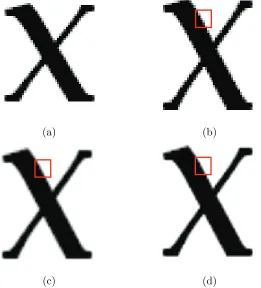
(a) (b)

(c) (d)

Figure 2.12: Comparison between common used interpolation methods. (a) the original LR image with size 53×49, the interpolated results of HR image with size 176×144 by using (b) nearest neighbor, (c) bilinear and (d) bicubic. In order to have a clear view of the original LR image, it has been shown in the same size as the other three images.

the visual distortion caused by the fractional interpolation ratio (Fig.2.12). Instead

of copying the neighboring pixels (which often results in jaggy images), these two

interpolation methods utilize the surrounding pixels to produce a smoother scaling at

edges (Fig.2.12 (c) and (d)). The constructed HR pixels are generated by using 2 linear

(42)

A

B

C

D

A

P

1

B

P

C

P

₂

D

W

H

Figure 2.13: The working principle of bilinear interpolation.

LR pixels can be constructed by bilinear interpolation. Referring to Fig.2.13, A,B,C

and D are four LR pixels and located at the corners of one texture area at positions (1,1),(1, W),(H,1) and (H, W), respectively. P is the targeted HR pixel at position (i, j). The first linear interpolation is carried out along the x axis and the pixels P1

and P2 at position(1, j) and (H, j) are obtained by

P1−A

j = B−A

W P2−C

j = D−C

W

(2.11)

Then, the second linear interpolation is carried out by using the pixelsP1 and P2.

P−P1 i =

P2−P1

H (2.12)

Substituting Eq.2.11 into 2.12 we get,

P = 1

HW [A(W −j)(H−i)+Bj(H−i)+Ci(W −j)+Dji] (2.13)

Similarly, all HR pixels among these four LR pixels can be interpolated.

In terms of performance, bicubic interpolation produces less blurring of edges and

other distortion artifacts in comparison to bilinear interpolation, but it is more

com-putationally demanding. Instead of using four pixels, bicubic interpolation fits a series

of cubic polynomials to the intensity values contained in a 4×4 array of LR pixels

surrounding the target HR pixel. It is also carried out in two steps. First, four

cu-bic polynomials (f(1), f(2), f(3) and f(4)) are fitted to four HR pixels along the

y-direction (the choice of starting direction is arbitrary). Next, these four HR pixels

are used to fit another cubic polynomial (F(1)) in the x-direction based on the

(43)

position can be obtained (Fig.2.14). Since the polynomial used in the bicubic

interpo-lation algorithm can have a significant impact on the accuracy and visual quality of the

interpolated image, splines as piecewise polynomial functions are often used.

f(1) f(2) _f(3)

f(4)

F(1)

Intensity level of pixel Target HR

pixel

Figure 2.14: The working principle of bicubic interpolation.

Different from other types of SR methods, interpolation-based SR approaches gain

their popularity in real-time applications mainly due to their computational simplicity

and they have lower requirements on the number of input LR images. Therefore,

interpolation-based SR approaches are suitable for applications with single input single

image where only one degraded LR image is available at the input terminal. They

have a good performance on smooth areas (low-frequency areas), but, work poorly on

edges (high-frequency areas) [52]. This is a common drawback of the conventional

interpolation methods where they cannot fully exploit the scene content during the

interpolation process, and consequently they are prone to blur high frequency details

(edges). In order to overcome these weaknesses, in [4], Li and Orchard proposed an

edge-directed interpolation algorithm for nature images. The interpolation algorithm

is composed of two steps, firstly, the local covariance coefficients of LR image are

estimated and then based on the geometric duality between the LR covariance and the

HR covariance, these estimated coefficients are used to steer the interpolation process.

Plenty of simulation results were used to demonstrate the effectiveness of the

edge-directed interpolation algorithm over conventional linear interpolations. In [5], a

small-kernel bilateral filter was proposed to implement image SR based on a novel maximum

Depth-Map-Assisted Texture and Depth Map Super-Resolution