Bayesian system identification of dynamical systems using large sets of training data: A MCMC solution

Bayesian system identi

fi

cation of dynamical systems using large sets

of training data: A MCMC solution

P.L. Green

1

Department of Mechanical Engineering, University of Sheffield, Mappin Street, Sheffield S1 3JD, United Kingdom

a r t i c l e i n f o

Article history: Received 17 April 2015 Accepted 17 September 2015 Available online 25 September 2015

Keywords:

Nonlinear system identification Markov chain Monte Carlo Bayesian inference Smooth data annealing Big data

a b s t r a c t

In the last 20 years the applicability of Bayesian inference to the system identification of structurally dynamical systems has been helped considerably by the emergence of Markov chain Monte Carlo (MCMC) algorithms–stochastic simulation methods which alleviate the need to evaluate the intractable integrals which often arise during Bayesian analysis. In this paper specific attention is given to the si-tuation where, with the aim of performing Bayesian system identification, one is presented with very large sets of training data. Building on previous work by the author, an MCMC algorithm is presented which, through combing Data Annealing with the concept of‘highly informative training data’, can be used to analyse large sets of data in a computationally cheap manner. The new algorithm is called Smooth Data Annealing.

&2015 The Authors. Published by Elsevier Ltd. This is an open access article under the CC BY-NC-ND license (http://creativecommons.org/licenses/by-nc-nd/4.0/).

1. Introduction

1.1. A Bayesian approach

Bayesian inference involves assessing the relative plausibility of a set of model structures M= {4 41, 2,…} – as well as the

parameters_θ∈Θ⊂N_{θwithin each model–using a combination} of one's prior knowledge and a set of training data,+. By virtue of influential papers such as [1] it is now well-established in the structural dynamics community that both levels of inference (parameter estimation and model selection) can be addressed via the sequential application of Bayes’theorem:

P P P

P

, ,

1

θ θ θ

( | ) = ( | ) ( | )

( | ) ( )

+ 4 + 4 4

+ 4

P P P

P . 2

( | ) = ( | ) ( )

( ) ( )

4 + + 4 4

+

Evaluation of Eq.(1)requires the definition of the prior, P( |θ4), and the likelihood,P(+|θ,4). The prior is a subjective probability distribution which describes one's knowledge of the parameters before the data was known. The likelihood describes the prob-ability of witnessing the data according to model, 4, with

parameters, θ. As such, the likelihood is defined by a‘ prediction-error model’ (see [2] for a comprehensive discussion). The de-nominator of Eq. (1) – the‘model evidence’ – is a normalising constant which ensures that P( |θ+ 4, )integrates to unity. Suc-cessful evaluation of Eq. (1) gives one the posterior parameter distribution, which describes the probability of parameter vector,

θ, given the training data,+, and the chosen model structure,4. With regard to Eq. (2), P(4) is a probability mass function which describes one's prior belief in model 4, P(+) is a nor-malising constant andP(+|M)is equal to the evidence term on the denominator of Eq.(1). P(4 +| ) is a distribution describing the relative probability of different competing model structures con-ditional on the data, +. One of the advantages of the Bayesian approach to model selection is that overly complex models tend to be assigned relatively low probabilities, thus preventing over-fi t-ting (see[3–5]for more information). Furthermore, via Eqs(1) and (2), one is able to quantify and propagate the inevitable un-certainties involved in the parameter estimation and model se-lection processes.

1.2. Why MCMC?

It is often the case that one wishes to generate samples from

P( |θ+ 4, )as part of a Monte Carlo analysis. With the geometry of the posterior parameter distribution often being fairly complex, this is usually impossible to achieve using well-known methods such as inverse transform sampling. Additionally, Monte Carlo methods such as importance sampling and rejection sampling are difficult to apply as the density of the posterior parameter dis-tribution tends to be concentrated in a small region of the Contents lists available atScienceDirect

journal homepage:www.elsevier.com/locate/probengmech

Probabilistic Engineering Mechanics

http://dx.doi.org/10.1016/j.probengmech.2015.09.010

0266-8920/&2015 The Authors. Published by Elsevier Ltd. This is an open access article under the CC BY-NC-ND license (http://creativecommons.org/licenses/by-nc-nd/4.0/). E-mail address:[email protected]

1

parameter space relative to the prior. Furthermore, the model evidence–which is found by integrating the posterior parameter distribution across the entire parameter space–is often difficult to obtain in a closed-form manner and, due to the large computa-tional cost involved, cannot usually be evaluated numerically.

Markov chain Monte Carlo (MCMC) methods involve the evo-lution of an ergodic Markov chain whose stationary distribution is

proportionalto the posterior parameter distribution. By allowing one's Markov chain to become stationary, MCMC can be used to generate (dependent) samples from P( |θ+ 4, ) while cir-cumventing the need to calculate the model evidence.‘Traditional’

methods include the well-known Metropolis [6] and Hybrid Monte Carlo algorithms[7]. Presently, more advanced MCMC al-gorithms are available which are able to generate samples from the posterior parameter distributionandestimate the model evi-dence/generate samples from the posterior model distribution simultaneously–these include Reversible Jump MCMC[8], Tran-sitional MCMC (TMCMC) [9], Nested Sampling [10]and Asymp-totically Independent Markov Sampling (AIMS) [11]. TMCMC in particular has become popular within the context of mechanical engineering, as it is able sample from distributions with complex geometries and is suitable for parallelisation[12].

Of specific relevance here is the concept of combining MCMC methods with the well-known Simulated Annealing algorithm

[13]. This involves using MCMC to target a sequence of distribu-tions defined by

P , P , j 1, 2, ,N ₃

j θ θ j θ

πβ( ) ∝ (+| 4)β ( |4) = … β _{( )}

where

0=β1<β2< ⋯ <βNβ=1 ( )₄

The result is that, by increasing

β

(the inverse temperature), one is inducing a gradual transition from the prior to the posterior parameter distributions. This technique has proved to be ex-tremely useful and forms a fundamental part of the TMCMC[9]

and AIMS[11]algorithms (as well as many others).

It is important to note that the strictly increasing sequence of

β

values–the annealing schedule–is crucial to the success of any MCMC algorithm which targets the sequence of distributions de-scribed by Eq.(3).

1.3. Motivation

The current paper is motivated by the situation where, as part of some collaborative work, one is presented with a very large set of training data from which the relative probability of various parameters/models are to be inferred (this is sometimes referred to as a‘Big Data’ issue). In such situations one oftenfinds that, despite the savings that can be achieved via parallelisation, the computational cost of MCMC dictates that only a small subset of the_‘full_’data can be utilised.

A possible solution to this problem is to use the Data Annealing algorithm[14]. Noting that, when employing a variant of Simu-lated Annealing, one is essentially using

β

to modulate (and in-crease) the in_fluence of the data on the target distribution, Data Annealing achieves a similar result simply via the gradual in-troduction of data points into the likelihood. This involves tar-geting the distribution

P N1 , P 5

θ θ θ

π( ) ∝ (+ | 4) ( |4) ( )

where N , , ,

N

1 = { 1 2 … }

+ + + + , using MCMC (a standard Metropolis

update was employed in[14]). Once a sufficient number of sam-ples have been generated,Ncan then be increased such that ad-ditional data points are included in the likelihood. This process is repeated until the statistical properties of one's parameter

estimates are judged to have converged. To ensure efficient MCMC performance a proposal density can be chosen whose covariance matrix (assuming a Gaussian proposal is being utilised) is a frac-tion of the distribufrac-tion which was most recently targeted. Alter-natively, as demonstrated in [14], it is possible to achieve sa-tisfactory results simply by using a heavy-tailed proposal dis-tribution. While Data Annealing tends to be fast (as the model does not have to reproduce the entire set of data every time a sample is generated), one has little control over the rate at which theinformationin the data is introduced into the likelihood.

A second option would be to utilise the approach described in

[15], where the approximate information content of data sets was measured. This can then allow one to select a small, highly in-formative subset of data from which to infer parameter estimates. This is achieved byfirst writing the posterior parameter para-meter distribution as

P( |θ+ 4, ) ∝exp( − ( ))Jθ ( )6

and employing a second order Taylor series expansion about the most-probable parameter estimate, θ^, to gain

A

J J 1

2 T 7

θ θ Δθ Δθ ( ) ≈ (^) +

( )

where A= ∇∇ (J θ^)and Δθ=θ−θ^. From this a Gaussian approx-imation of the posterior can be obtained

⎛ ⎝

⎜ ⎞

⎠ ⎟

A

A P

Z Z

, 1exp 1

2 ,

2 .

8

T N

θ Δθ Δθ π

*( | ) = − = ( )

| | ( )

θ + 4

The information content of this distribution can then be measured using the Shannon entropy:

⎛ ⎝

⎜ ⎞

⎠ ⎟

A

S P , logP , d 1 e

2log 2

9 N

∫

θ θ θ π

= − *( | ) *( | ) = ( )

| | ( )

θ

+ 4 + 4

whose properties as an information measure are well known[16]. Eq.(9)can then be used to estimate the influence of the available training data on the information content of the posterior.2 A drawback of this method is that it relies on one knowing the lo-cation of θ^before the analysis can begin.

The algorithm proposed in the current paper encompasses elements from Data Annealing and the concept of highly in-formative training data. It is designed to overcome the drawbacks of both the afore-mentioned methodologies and is suitable for dynamical models (see[17]for a solution which can be applied to static models).

2. Smooth data annealing

2.1. Basic methodology

As in the previous section, N

1

+ denotes the data

, , , N

1 2

{+ + … + }. With Smooth Data Annealing (SDA), one begins by targeting the distribution:

P P ₁₀

N N

1 1

jθ θ j θ

πβ( |+ ) ∝ (+ | )β ( ) _{( )}

where N is a predefined integer, N

1

+ is a small subset of the available training data (choice ofNis discussed inSection 4) and, from now on, dependence on model structure is omitted. By in-creasing

β

one can then ‘anneal in’ the data N

1

+ in the usual manner. Once β=1then one can choose to add an additionalk

data points and redefine the target distribution as

P P P . ₁₁

N k N

N N k

1 1 1

j θ θ θ j θ

πβ( |+ + ) ∝ (+ | ) (+ ++ | )β ( ) _{( )}

(assuming thatP N

1θ

(+ | )andP(+NN k++1| )θ are mutually independent).

This process can then be repeated until certain criteria are met. SDA therefore has all the advantages of Data Annealing, while also giving the user complete control of the rate at which the in_fluence of the data is introduced. The choice of annealing schedule is discussed in the next section.

2.2. Constant entropy variation

Here it is hypothesised that the optimum annealing schedule is one in which the information content, measured using the Shan-non entropy, varies at a constant rate. This allows the concept of only using highly informative training data[15]to become an in-herent feature of SDA–data which has little influence with regard to one's parameter uncertainty is annealed in quickly, thus al-lowing the algorithm to focus on the data which is‘information rich'.

For the remaining part of this section it is advantageous for the target PDF (Eq. (11)) to be written in the following form:

J J J

Z exp

12

j L L P

π= ( −β

^

− − )

( )

where

J_L ln P _NN k , J ln P ₁₃

L N

1 1

(

θ

)

(

θ

)

^ _{= − ( | ) = − ( | )}

( )

+ +

+ +

and JP is the negative log-prior.3 Furthermore, the target dis-tribution is written as π=π⁎/Z _{such that Z is the normalising}

constant of the unnormalised distribution π⁎_.

Before further discussion it is convenient to first derive the following properties:

d

d J

dZ

d Z J

d

d J J

E E ,

14

j L j L j L L

π

β π β

π β π = −^ = − [^] = ( [^] −^) ( ) ⁎ ⁎

(seeAppendix A). The Shannon entropy of the target distribution

is

S=β_jE[J^_L] +E[ ] +J_L E[ ] +J_P ln( )Z ₍₁₅₎

such that the task is to evaluate

dS d d d J d d J d d Z

E E ln

16

j j

(

j L

)

j

(

L

)

j

(

)

β = β β [ β β

^_{] + [ ] + ( )}

( )

(noting theJPis not a function of

βj

). Using the properties in Eq.

(14), thefirst term in Eq.(16)can be evaluated as follows:

d

d J J

d

d J d

E E

17 j

j L L j

j L

(

)

∫

θ

β β [ β β π

^_{] = [}^_{] +} ^

( )

d

dj jEJL EJL j E JL EJL 18

2 2

(

)

(

)

β β [ β

^

] = [^] + [ ] − [ ]

( )

d

dβ_j

(

βjE[JL

)

EJL βjVarJL . ₁₉ ^_{] = [}^_{] − (}^₎

( )

The second term in Eq.(16)is

d

d J

d

d J d

E

20

j

(

L

)

j

∫

L

θ

β [ ] = β π _{( )}

d

dβ_j

(

E[ ] =JL

)

∫

JL( [EJL JL πdθ ₂₁ ^

] −^)

( )

d

d j EJL EJL EJL EJ JL L 22

(

)

β [ ] = [ ] [ ^

] − [ ^]

( )

d

dβ_j

(

E[ ] = −JL

)

Cov(J JL, L ₂₃

^₎

( )

whereCov(J JL,^L)is the covariance betweenJLand J^L. Finally, the third term in Eq.(16)is

d

d lnZ Z Z J

1 E

24

j

(

L

)

(

)

β = − [

^ ]

( )

d

dβ_j

(

lnZ

)

= −E[JL . ₂₅

^_]

( )

Combining Eqs.(19), (23) and (25) onefinds that

dS

dβj jVarJL CovJ JL, L . 26

β

= − (^) − ( ^)

( )

Consequently, if the algorithm is currently using the value

βj

and one wishes to‘anneal in’new data with a constant change in the Shannon entropy,ΔS, then

βj

þ1should be selected according to

S

J J J

Var Cov ,

.

27

j j

j L L L

1

β β

β

= − Δ

(^) + ( ^) _{( )}

+

If one considers the initial stages of the algorithm (where only the first set of data is being annealed) then Eq.(27)simplifies to

S J Var . 28 j j j L 1 β β β

= − Δ

(^) ( )

+

It is important to note that, to avoid numerical issues, it is often beneficial to initiate the annealing schedule by selecting a value of

β

which is close to, but not equal to zero. By choosing a small initial

β

one is ensuring that the geometry of thefirst target dis-tribution is similar to that of the prior (this will allow efficient sampling from the target using MCMC). A more sophisticated approach could involve using the methods described in [15] to estimate the Shannon entropy of thisfirst target distribution, thus ensuring that this initial choice of

β

has not led to a large change in the Shannon entropy. Throughout this work it was found that initially setting _β=1_×10−4_{yielded acceptable results.}

Table 1

System identification of a simulated Duffing oscillator: true parameter values and moments of prior distributions.

Parameter True value Prior mean Prior standard deviation Units

k 100 150 30 N/m

c 0.05 0.02 0.02 N s/m

k3 100,000 40,000 20,000 N/m3

s 0.005 0.0045 0.002 –

2.3. Does data reduce entropy ?

Typically one would chooseΔSto be negative because, as the influence of the data is increased, one wishes to see a reduction in parameter uncertainty. Referring to Eq.(28)it is clear that, when the algorithm is initialised,

βj

þ1must always be larger than

βj

as

S

Δ is negative. However, in the general case (Eq. (27)), if the covariance betweenJLand J^L is negative then by imposing that

S 0

Δ < one can actually select a value

βj

þ1which islowerthan

βj

. This prompts one ask whether the addition of new data will ne-cessarily reduce parameter uncertainty.

Intuitively the answer appears to be no – parameter un-certainty could increase in the situation where the new data contradicts the information in the old data (which is also when

J J

Cov(L,^L)will be negative). To address this issue one can use the well-known result

E Var[ ( |θ+)] =Var( ) −θ Var E( [ |θ+]) (29)

which states that,on average, the variance of the posterior must be less than that of the prior. Consequently, if new data does con-tradict the information in the old data, one can simply allow the Shannon entropy to increase (safe in the knowledge that, on average, the increasing influence of more data must ultimately lead to a decrease in parameter uncertainty). The key is to ensure that the Shannon entropy always remains between some

pre-defined limits, such that the transition from prior to posterior is still conducted in a gradual manner.

To be specific,

βj

þ1should be selected according to

S

J J J

Var Cov , ₃₀

j j

j L L L

1

β β

β

= − Δ

(^) + ( ^) _{( )}

+

butsubject to the conditions that

S S S

1, ₃₁

j j 1 lim lim

β <β₊ ≤ − Δ < Δ < Δ _{( )}

where ΔSlimis defined by the user.

3. Algorithm

The method by which SDA anneals in the data +NN k++1is

sum-marised here using pseudo-code:

Setj¼1, βj=βinitial

While βj <1

○ Generate samples_{θ( )1,_…,_θ(Ns)_}from N k _{exp J} j L

1

j θ

πβ( |+ +) ∝ ( −β^ J_L J_P

− − ) using MCMC

○ Estimate Var(J^L)andCov(J^L,JL)

○ Set j j

S

J J J

1

Var Cov ,

j L L L

β =β − β +

Δ

(^) + ( ^)

subject to the conditions that

1

j j 1

β <β₊ ≤ and −ΔSlim < Δ < ΔS Slim

0 100 200 300 400 500 600 700 800 900 1000

−0.08 −0.06 −0.04 −0.02 0 0.02 0.04 0.06 0.08

Data Point

[image:4.595.143.465.59.208.2]

x (m)

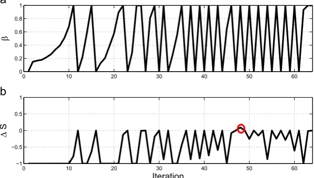
Fig. 1.Training data for the system identification of a simulated Duffing oscillator. Dashed lines indicate the segments of data which were used in the SDA algorithm. (For interpretation of the references to color in thisfigure caption, the reader is referred to the web version of this paper.)

0 10 20 30 40 50 60

0 0.2 0.4 0.6 0.8 1

β

0 10 20 30 40 50 60

−1 −0.5 0 0.5 1

Iteration

Δ

S

[image:4.595.142.466.250.434.2]

○ j=j+1

End

IfStopping criteria met ○ Terminate algorithm

else

○ Add more data by setting N=N+k

End

It should be noted that when samples are being generated from N k

1

j θ

πβ( |+ + ), any MCMC algorithm can be employed. While the

Metropolis algorithm was utilised in the current paper, it should be relatively easy to incorporate more advanced MCMC methods as part of SDA. One could, for example, combine SDA with TMCMC

[9].

4. Example 1–simulated data

As an initial example, a time history of displacement dataxwas

0 10 20 30 40 50 60

50 100 150 200

E[k] (N/m)

0 10 20 30 40 50 60

0.02 0.04 0.06

E[c] (Ns/m)

0 10 20 30 40 50 60

0 5 10 15x 10

E[k

3

] (N/m

3 )

0 10 20 30 40 50 60

4.5 5 5.5

6x 10

Iteration

E[

σ

]

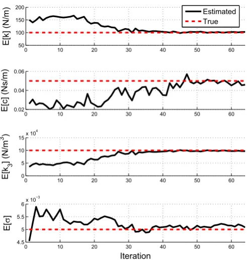
[image:5.595.37.283.54.313.2]

Estimated True

Fig. 3.Parameter estimation of a simulated Duffing oscillator: convergence of parameter estimates to true values as SDA algorithm is run.

0 10 20 30 40 50 60

0 20 40

Std(k) (N/m)

0 10 20 30 40 50 60

0 0.01 0.02

Std(c) (Ns/m)

0 10 20 30 40 50 60

0 1 2 3x 10

Std(k

3

) (N/m

3 )

0 10 20 30 40 50 60

0 1 2 3x 10

Iteration

Std(

σ

[image:5.595.304.550.58.254.2]

)

Fig. 4.Parameter estimation of a simulated Duffing oscillator: reduction of pos-terior parameter standard deviation as SDA algorithm is run.

0 10 20 30 40 50 60 70

−1 −0.8 −0.6 −0.4 −0.2 0 0.2 0.4 0.6 0.8 1

Iteration

Cor(k,k

3

)

Fig. 5.Parameter estimation of a simulated Duffing oscillator: variation of the (normalised) correlation coefficient betweenkandk3as training data is added.

0 2 4 6 8 10 12 14 16 18 20

50 100 150 200

E[k] (N/m)

0 2 4 6 8 10 12 14 16 18 20

0.02 0.03 0.04 0.05 0.06

E[c] (Ns/m)

0 2 4 6 8 10 12 14 16 18 20

4 6 8 10 12x 10

E[k

3

] (N/m

3

)

0 2 4 6 8 10 12 14 16 18 20

4.5 5 5.5

6x 10

Iteration

E[

σ

]

[image:5.595.305.551.304.593.2]

Estimated True

[image:5.595.37.282.350.609.2]

created by simulating the response of a Duffing oscillator:

mx¨ +cẋ +kx+k x3 3=F, (32)

whereFwas a Gaussian white noise force. The time history was then artificially corrupted with Gaussian measurement noise of standard deviations. The massmwas set equal to 0.1 and was assumed to be known. The parametersc,k,k3andswere left as parameters to be estimated. Throughout this example Gaussian

distributions, truncated at zero, were used as priors. To study the convergence properties of SDA, the mean values of the priors were deliberately set to be different from the true parameter values (see

Table 1).

The‘full’set of training data consisted of 1000 displacement measurements–this is shown inFig. 1. Of this set, the data was introduced to SDA in segments of 50 points at a time (these seg-ments of data are separated by dashed red lines inFig. 1).

Setting ΔSlim=1the SDA algorithm was run, generating 1000

samples at each iteration.Fig. 2shows the resulting variation in

β

and ΔS. It should be noted that a new segment of data is in-troduced every time

β

has reached a value of one. Each point on the horizontal axis ofFig. 2therefore represents an iteration of the algorithm (not the introduction of a new segment of data). It is clear that, after 35 iterations (where 350 points have been ana-lysed), the remaining data appears to be relatively uninformative and the desired change in Shannon entropy can be realised by instantly setting β=1. It is interesting to observe that, in the al-gorithm's 48th iteration (marked with a red circle in Fig. 2), a slight increase in Shannon entropy occurred. For the most part however, for this simple example, it appears that the introduction of more data has consistently reduced parameter uncertainty.

As mentioned previously, one can simply allow the SDA algo-rithm to run until certain criteria are met (so long as training data is still available).Fig. 3shows how the posterior mean estimates of each parameter converged to their true values while, inFig. 4, one can see how the posterior standard deviation of each parameter estimate reduced while additional data was being analysed. Fur-thermore, as MCMC can be used to approximate the posterior parameter covariance matrix [18], one can also track parameter correlations as data is added.Fig. 5shows how, as training data is annealed in, the well-known negative correlation between the linear and nonlinear stiffnesses becomes apparent.

This same data set was then analysed using the original Data Annealing algorithm, such that the relative performance of the two methods could be assessed. The same prior and segments of data were used.Figs. 6and7show how the posterior mean and standard deviation estimates evolved as more data was analysed.

0 2 4 6 8 10 12 14 16 18 20

0 10 20

Std(k) (N/m)

0 2 4 6 8 10 12 14 16 18 20

0 0.01 0.02

Std(c) (Ns/m)

0 2 4 6 8 10 12 14 16 18 20

0 1 2x 10

Std(k

3

) (N/m

3

)

0 2 4 6 8 10 12 14 16 18 20

0 2 4 6x 10

Iteration

Std(

σ

[image:6.595.312.557.56.327.2]

)

Fig. 7.Parameter estimation of a simulated Duffing oscillator: reduction of pos-terior parameter standard deviation as the Data Annealing algorithm is run.

0 100 200 300 400 500 600 700 800 900 1000

100 102 104

k (N/m)

0 100 200 300 400 500 600 700 800 900 1000

0.04 0.045 0.05 0.055

c (Ns/m)

0 100 200 300 400 500 600 700 800 900 1000

9.6 9.8

10x 10

k

3

(N/m

3

)

0 100 200 300 400 500 600 700 800 900 1000

4.8 5 5.2 5.4x 10

σ

Fig. 8.Evolution of Markov chains used in the Data Annealing algorithm.

[image:6.595.46.294.58.343.2]

While these results look promising, it was found that they were based on relatively few independent samples ofθ. This is because the algorithm was unable to appropriately adapt the size of its proposal density as the geometry of the posterior altered– this resulted in the acceptance ratio dropping to below 10% once all 1000 data points were being analysed (seeFig. 8for example). The crucial point here is that Data Annealing can be a very efficient algorithm, just so long as it is tuned appropriately. Choosing smaller segments of data could, for example, have allowed the algorithm to realise a higher acceptance ratio. The advantage of SDA is that it is relatively insensitive to this sort of tuning. If very small segments of data are used then, as they will contain less

0 200 400 600 800 1000 1200 1400 1600 1800 2000

−1 −0.8 −0.6 −0.4 −0.2 0 0.2 0.4 0.6 0.8 1

Data Point

Relative Acceleration (m/s

[image:7.595.128.453.60.182.2]

2)

[image:7.595.306.552.236.457.2]

Fig. 10.Training data for the system identification of a rotational energy harvester. Dashed red lines indicate the segments of data which were used in the SDA algorithm. (For interpretation of the references to color in thisfigure caption, the reader is referred to the web version of this paper.)

Table 2

System identification of rotational energy harvester: moments of prior distributions.

Parameter Prior mean Prior standard deviation Units

c 170 50 N s/m

Fc 10 5 N

α 100 100 s/m

s 0.07 0.03 –

0 50 100 150

0 0.2 0.4 0.6 0.8 1

β

0 50 100 150

−1 −0.5 0 0.5 1

Iteration

Δ

S

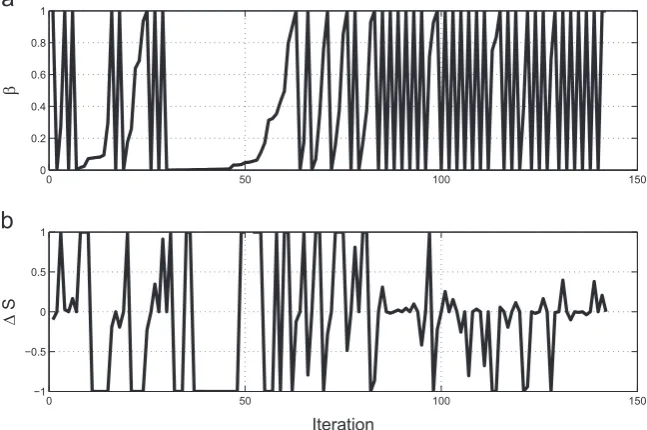
Fig. 11.Parameter estimation of a rotational energy harvester: variation of (a) inverse temperature and (b) the change in Shannon entropy as training data is added to the SDA algorithm.

0 50 100 150

0 100 200 300

E[c] (Ns/m)

0 50 100 150

0 20 40

E[F

c

] (N)

0 50 100 150

0 500 1000

E[

α

] (s/m)

0 50 100 150

0 0.05 0.1

E[

σ

[image:7.595.31.284.267.326.2]

]

[image:7.595.131.455.506.721.2]

information, SDA will move through them quickly. If very large segments of data are used then SDA will ensure that the in-formation contained within will be introduced slowly, and no dramatic changes in the geometry of the posterior will occur.4_This

property therefore gives the user greatflexibility when selecting the size of each data segment. Throughout this paper segments were chosen on the basis that they appeared to capture some of the system's dynamic behavior_–this led to satisfactory results in both examples.

5. Example 2–experimental data

In this section SDA is applied to experimentally obtained data.

The system in question is a vibrational energy harvesting device which, via a ball-screw mechanism, is able to convert low fre-quency translational motion into high frefre-quency rotational mo-tion. Originally tested at the University of Southampton's Institute of Sound and Vibration Research, only a very brief description of the device and experimental procedure is given here–more in-formation can be found in the references [19,20]. It should be noted that the data from this experiment can be found in the electronic supplementary material of the paper[22].

A schematic of the energy harvester is shown inFig. 9. As the device experiences base motion, the mass,m, oscillates relative to the outer frame. This translational motion is then converted into rotational motion via a ball screw. The response of device is strongly affected by friction (as a result of the coupling between the mass and the ball screw). Building on other work on rotational energy harvesters[21], the hyperbolic tangent model was used to model friction effects in the device. Defining z=x−y as the re-lative displacement between the mass and the base, the proposed

0 50 100 150

0 20 40 60

Std(c) (Ns/m)

0 50 100 150

0 2 4 6

Std (F

c

) (N)

0 50 100 150

0 50 100 150

Std(

α

) (s/m)

0 50 100 150

0 0.02 0.04

Iteration

Std(

σ

[image:8.595.181.426.58.290.2]

)

Fig. 13.Parameter estimation of a rotational energy harvester: convergence of posterior standard deviation parameter estimates as SDA algorithm is run.

100 110 120

0 20 40 60 80 100 120 140 160 180

c (Ns/m)

Frequency of Samples

11 11.5 12 12.5

0 20 40 60 80 100 120 140 160 180 200

F

c (N)

70 80 90 100 110

0 50 100 150 200 250

α (s/m)

0.090 0.095 0.1

50 100 150 200 250 300

σ

Fig. 14.Parameter estimation of a rotational energy harvester: histograms of SDA results.

[image:8.595.142.464.330.510.2]

equation of motion is therefore

Mz¨ +b zm ̇ +kz+Fctanh(αż) = −my¨ (33)

where

⎜ ⎟ ⎜ ⎟

⎛

⎝ ⎞⎠ ⎛⎝ ⎞⎠

M m J

l b l c

2

, 2 ,

34

m m

2 2

π π

= + =

( )

Jis the moment of inertia of the system andlis the ball-screw lead. The parameters to be estimated werec,Fc,

α

andswhere, as be-fore,sis the likelihood standard deviation.

The‘full’training data consisted of 2000 points of relative ac-celeration time history (z¨). This was‘fed’into SDA in segments of 50 points at a time (as shown inFig. 10). The parameters of SDA were the same as in the previous example while, again, Gaussian priors truncated at zero were utilised (seeTable 2). The prior was selected based on several static tests which had already been conducted–see[20]for more details.

The variation of

β

and Shannon entropy is shown inFig. 11. It is clear that, relative to the previous example, this problem was more challenging (as many more positive values of Shannon entropy were realised). It is also interesting to note that, between the 31st and 63rd iterations of the algorithm, a large amount of time has been spent annealing in a single segment of data. This was actually the 9th subset of data which, as can be seen from fromFig. 10, is where the relatively high amplitude portion of the training data begins.

For the sake of completeness the convergence of the mean and standard deviation parameter estimates is shown inFigs. 12and13

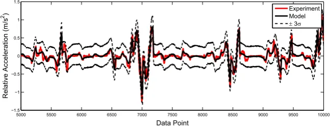
whileFig. 14 shows histograms of the resulting MCMC samples. Using the MCMC samples to propagate parameter uncertainties, Monte Carlo simulations were conducted to compare the model response with a new set of test data.Fig. 15shows that the model is able to replicate the data accurately.

6. Conclusions

Presented here is a novel MCMC algorithm – Smooth Data Annealing (SDA) – which is designed to be used in situations where one is conducting Bayesian system identification of dyna-mical models using large sets of training data. The algorithm is designed to ‘absorb’data in a smooth and continuous manner, ensuring that the resulting change in the Shannon entropy of one's target distribution remains within predefined limits. This allows the algorithm to quickly move through training data which is re-latively uninformative, and concentrate on that which has a greater influence on one's parameter estimates.

Acknowledgements

The author would like to thank Dr. Mehdi Hendijanizadeh, Mr. Luigi Simeone and Professor Stephen Elliott from the University of Southampton's Institute of Sound and Vibration Research for providing the data used in the second example.

The author would also like to acknowledge funding from the EPSRC programme Grant‘Engineering Nonlinearity’EP/K003836.

Appendix A. Deriving Eq. (14)

Recalling that

J J J

Z Z

exp

A.1

j L L P

π= ( −β π

^ _{− − )}

=

( )

⁎

then thefirst property can be derived by

d d

d

d J J J J J J J

J

exp exp

. A.2

j j j L L P L j L L P

L

(

)

(

)

π

β β β β

π

= − ^ − − = −^ − ^ − −

= −^ ( )

⁎

⁎

This allows the second property to be derived by

dZ d

d

d d

d

d d J d Z J d

Z JE . A.3

j j j L L

L

∫

θ

∫

θ

∫

θ

∫

θ

β β π

π

β π π

= = = − ^ = − ^

= − [^] ( )

⁎ ⁎ ⁎

Finally then, the third property can be derived by

d d

d

d Z J Z

dZ

d J J

J J

E

E .

A.4

j j L j L L

L L

1

(

)

π

β β π π

π

β π π

π

= ( ) = −^ − = −^ + [^]

= [^] −^

( )

⁎ −

References

[1]J.L. Beck, L.S. Katafygiotis, Updating models and their uncertainties. I. Bayesian statistical framework, J. Eng. Mech. 124 (4) (1998) 455–461.

[2]E. Simoen, C. Papadimitriou, G. Lombaert., On prediction error correlation in Bayesian model updating, J. Sound Vib. 332 (18) (2013) 4136–4152. [3]D.J.C. MacKay., Bayesian interpolation, Neural Comput. 4 (3) (1992) 415–447. [4]D.J.C. MacKay, Information Theory, Inference and Learning Algorithms,

Cam-bridge University Press, CamCam-bridge, UK, 2003.

[5]M. Muto, J.L. Beck, Bayesian updating and model class selection for hysteretic structural models using stochastic simulation, J. Vib. Control 14 (1–2) (2008) 7–34.

[6]N. Metropolis, A.W. Rosenbluth, M.N. Rosenbluth, A.H. Teller, E. Teller., Equa-tion of state calculaEqua-tions by fast computing machines, J. Chem. Phys. 21 (1953) 1087.

[7]S. Duane, A.D. Kennedy, B.J. Pendleton, D. Roweth., Hybrid Monte Carlo, Phys. Lett. B 195 (2) (1987) 216–222.

[8]P.J. Green, Reversible jump Markov Chain Monte Carlo computation and

5000 5500 6000 6500 7000 7500 8000 8500 9000 9500 10000

−1.5 −1 −0.5 0 0.5 1 1.5

Data Point

Relative Acceleration (m/s

2)

Experiment Model

[image:9.595.131.455.59.183.2]

± 3σ

Bayesian model determination, Biometrika 82 (4) (1995) 711–732.

[9]J. Ching, Y. Chen, Transitional Markov Chain Monte Carlo method for Bayesian model updating, model class selection, and model averaging, J. Eng. Mech. 133 (7) (2007) 816–832.

[10]J. Skilling, Nested sampling for general Bayesian computation, Bayesian Anal. 1 (4) (2006) 833–859.

[11]J.L. Beck, K.M. Zuev, Asymptotically independent Markov sampling: a new Markov Chain Monte Carlo scheme for Bayesian inference, Int. J. Uncertain. Quant. 3 (5) (2013).

[12]P. Angelikopoulos, C. Papadimitriou, P. Koumoutsakos, Bayesian uncertainty quantification and propagation in molecular dynamics simulations: a high performance computing framework, J. Chem. Phys. 137 (14) (2012) 144103. [13] S. Kirkpatrick, D.G. Jr., M.P. Vecchi, Optimization by simmulated annealing,

Science 220(4598) (1983) 671–680.

[14]P.L. Green, Bayesian system identification of a nonlinear dynamical system using a novel variant of simulated annealing, Mech. Syst. Signal Process. 52 (2015) 133–146.

[15]P.L. Green, E.J. Cross, K. Worden, Bayesian system identification of dynamical systems using highly informative training data, Mech. Syst. Signal Process. 56 (2015) 109–122.

[16]C.E. Shannon, A mathematical theory of communication, ACM SIGMOBILE Mob. Comput. Commun. Rev. 5 (1) (2001) 3–55.

[17] N. Chopin, A sequential particlefilter method for static models, Biometrika 89 (3) (2002) 539–552.

[18]K. Worden, J.J. Hensman, Parameter estimation and model selection for a class of hysteretic systems using Bayesian inference, Mech. Syst. Signal Process. 32 (2012) 153–169.

[19] L. Simeone, M.G. Tehrani, S. Elliott, M. Hendijanizadeh, Nonlinear damping in an energy harvesting device, in: Proceedings of ISMA 2014 Iternational Con-ference on Noise and Vibration Engineering, Leuven, Belgium, 2014. [20] P.L. Green, M. Hendijanizadeh, L. Simeone, S.J. Elliott, Probabilistic modelling

of a rotational energy harvester, J. Intell. Mater. Syst. Struct.,http://dx.doi.org/ 10.1177/1045389X15573343, in press.

[21]I.L. Cassidy, J.T. Scruggs, S. Behrens, H.P. Gavin, Design and experimental characterization of an electromagnetic transducer for large-scale vibratory energy harvesting applications, J. Intell. Mater. Syst. Struct. 22 (17) (2011) 2009–2024.